Early Phase of the COVID-19 Outbreak in Hungary and Post-Lockdown Scenarios

Article

Early Phase of the COVID-19 Outbreak in Hungary and Post-Lockdown Scenarios

Gergely Röst¹ , Ferenc A. Bartha^1,∗ , Norbert Bogya¹, Péter Boldog¹, Attila Dénes¹ , Tamás Ferenci² , Krisztina J. Horváth¹, Attila Juhász^1,3, Csilla Nagy^1,3, Tamás Tekeli¹, Zsolt Vizi¹and Beatrix Oroszi¹

1 Bolyai Institute, University of Szeged, 6720 Szeged, Hungary; rost@math.u-szeged.hu (G.R.);

nbogya@math.u-szeged.hu (N.B.); boldogpeter@gmail.com (P.B.); denesa@math.u-szeged.hu (A.D.);

horvath.j.krisztina@nnk.gov.hu (K.J.H.); juhasz.attila@nfo.bfkh.gov.hu (A.J.);

nagy.csilla@nfo.bfkh.gov.hu (C.N.); tekeli@math.u-szeged.hu (T.T.); zsvizi@math.u-szeged.hu (Z.V.);

oroszi.beatrix@nnk.gov.hu (B.O.)

2 Physiological Controls Research Center, Óbuda University, 1034 Budapest, Hungary;

ferenci.tamas@nik.uni-obuda.hu

3 Department of Public Health, Government Office of Capital City Budapest, 1034 Budapest, Hungary

* Correspondence: barfer@math.u-szeged.hu

Received: 31 May 2020; Accepted: 26 June 2020; Published: 30 June 2020 Abstract:COVID-19 epidemic has been suppressed in Hungary due to timely non-pharmaceutical interventions, prompting a considerable reduction in the number of contacts and transmission of the virus. This strategy was effective in preventing epidemic growth and reducing the incidence of COVID-19 to low levels. In this report, we present the first epidemiological and statistical analysis of the early phase of the COVID-19 outbreak in Hungary. Then, we establish an age-structured compartmental model to explore alternative post-lockdown scenarios. We incorporate various factors, such as age-specific measures, seasonal effects, and spatial heterogeneity to project the possible peak size and disease burden of a COVID-19 epidemic wave after the current measures are relaxed.

Keywords: COVID-19; epidemic; Hungary; under-ascertainment; SARS-CoV-2; compartmental model; reproduction number; intervention; case fatality rate

1. Introduction

A cluster of pneumonia cases of unknown origin was detected in Wuhan city, the capital of Hubei Province, China, with a population of 11 million in December 2019. On 31 December 2019 China alerted the World Health Organization (WHO) China Country Office [1]. On 7 January 2020 the causative pathogen of the pneumonia outbreak was identified as a novel coronavirus, and, on 11 February, the WHO officially named the novel coronavirus as SARS-CoV-2 and the disease it causes as COVID-19.

SARS-CoV-2 infection quickly spread from China, where it emerged in December 2019, to Europe, where the first cases were confirmed on 24 January 2020 in France (where, later in April, COVID-19 was retrospectively confirmed for a patient hospitalized in late December 2019) [2,3]. Around the same time, on 27 January, the first infection in Germany was confirmed in Bavaria that led to a local outbreak. By February 19, 16 subsequent cases have been confirmed and 241 high-risk contacts have been identified via agile contact-tracing [4]. The first epidemic in Europe started in the Lombardy region of Italy with the first detection on 20 February 2020 [5]. The WHO Director-General declared the COVID-19 outbreak a Public Health Emergency of International Concern under International Health Regulations (2005) on 30January 2020 [6] and then a pandemic on 11 March 2020 [7]. By that time, the number of daily new cases of COVID-19 was over 100 in several countries, including Italy, France, and Germany.

Viruses2020,12, 708; doi:10.3390/v12070708 www.mdpi.com/journal/viruses

Containment measures started in mid-March in most of the EU-EEA countries, which included physical distancing measures such as school and workplace closures, cancellation of public events, restrictions of gatherings, and stay-at-home requirements as a response to the pandemic, aiming to reduce transmission of SARS-CoV-2. These measures reflect strong effort to suppress, or at least to slow down COVID-19. Some governments hesitated to mount a broad containment response quickly when the virus first emerged and there were also differences in the severity of restrictions they put in place at first. As a result, the peak daily incidence varied substantially between EU/EEA countries during the first COVID-19 pandemic wave [8].

The emergence of the new coronavirus in Hungary did not happen until early March. Phylogenetic analysis revealed multiple and parallel introduction of the virus into the country [9]. By that time, diagnosis and treatment, surveillance, epidemiological investigation, management of close contacts, and diagnostic testing were being developed and put in place. The strategy of Hungary was to suppress the epidemic to avoid the overload of the health care system and excess deaths, so they decided on fast and strong measures right after community transmission was established in Italy and a pandemic was declared by the WHO.

Here, we provide the first epidemiological and statistical study of the early phase of the COVID-19 outbreak in Hungary, focusing on the period 4 March–10 May. Our analysis provides insights to understand how the first wave transpired in the country, and shows that the timely non-pharmaceutical interventions were successful. Since the control measures are being progressively relaxed, to explore possible future scenarios, we employ an age structured compartmental model. The model allows us to investigate the impact of contact reductions, age-specific measures, seasonality, and spatial heterogeneity on the transmission dynamics, healthcare demand, mortality, and overall disease burden.

2. Materials and Methods

2.1. Epidemiological Report

During the last week of January 2020, the National Public Health Center (hereinafter NPHC) issued the surveillance protocol of COVID-19 cases that included the case definitions of COVID-19 cases. Until mid May, the protocol was updated four times as the relevant WHO and/or European Centre for Disease Prevention and Control (ECDC) guidance was revised. According to the Hungarian protocol, suspected cases were to be reported by physicians to the local health authority and NPHC, followed by compulsory testing, 14-day isolation and monitoring, case investigation, and contact tracing. A person with laboratory confirmation (detection of SARS-CoV-2 by polymerase chain reaction), irrespective of clinical signs and symptoms, was considered a confirmed COVID-19 case.

The primary data source regarding the COVID-19 outbreak in Hungary was the NPHC. Official announcements were published on a government hosted website [10] since 1 March, including epidemiological data, but not in a systematic way. The findings of our epidemiological analysis are detailed in Section3.1.

2.2. Statistical Analysis

Statistical analysis of the available surveillance data—such as case counts and death counts—is an indispensable tool during outbreak response. It can reveal the current situation objectively, shed light on the effect of past interventions, uncover non-obvious aspects of the outbreak, and produce forecasts.

It can also provide important input information to disease dynamics models.

This section summarizes the statistical analyses carried out, based on data from NPHC, during the early phase of the COVID-19 outbreak in Hungary, pointing out the most important tasks and methods.

All methods were implemented under theR statistical environment version 4.0.0 [11] using packages ggplot2 version 3.3.0 [12] for visualization, data.table version 1.12.8 [13] for data

manipulation and shiny version 1.4.0.2 [14] for creating an interactive dashboard to carry out epidemiological analyses online (available in Hungarian [15]).

The full source code of this dashboard and related analysis is available at [16].

2.2.1. Temporal Variation of the Effective Reproduction Number

Effective reproduction number (Rt), the average number of secondary cases per primary case for those primary cases who turn infectious on dayt, was tracked in real time based on the daily number of reported new cases using the methods of Cori et al. [17] and that of Wallinga and Teunis [18], among the several methods aimed to estimateR_t[19,20]. In brief, the method of Cori et al., is based on calculating the ratio of the actual number of infections on a day to the total infectiousness of all past cases on that day. Thus, it measuresR_tby assuming that infected individuals will infect in the future as if conditions remain unchanged. In contrast, the method of Wallinga and Teunis makes no such assumption; it uses a likelihood-based inference on the possible infection networks underlying the epidemic curve. The fundamental difference is that the method of Cori et al., solely uses past information (“backward looking approach”), due to which the result is sometimes called instantaneous reproduction number, while the Wallinga–Teunis method more closely corresponds to the concept of the usual definition of effective reproduction number; however, it requires future information in exchange (“forward looking approach”).

For a discussion on the relative merits of these two approaches, see [21,22]. The Wallinga–Teunis method was used with the addition of Cauchemez et al., who aimed to provide real-time estimation capability [23].

Both methods require—in addition to incidence data—information on the serial interval.

Depending on the used dataset, different estimations of the serial interval have been published:

a mean of 3.96 days was found in [24], and 6.6 days in [25]. Here, we assume an intermediate value following [26], where the mean and standard deviation (SD) of the serial interval were estimated at 4.7 days (95% CrI: 3.7, 6.0) and 2.9 days (95% CrI: 1.9, 4.9), respectively. (The serial interval is assumed to follow gamma distribution.) They also concluded that the serial interval of COVID-19 is close to or shorter than its median incubation period, which is coherent with our choice of parameters in the transmission dynamics model.

The estimation was carried out usingRpackagesR0version 1.2-6 [27,28] andEpiEstimversion 2.2-2 [17,29].

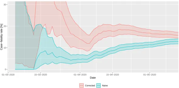
2.2.2. Adjusted Case Fatality Ratio

Case fatality rate (CFR) is defined as the (conditional) probability of death from a disease for those contracting the disease (for diseases where asymptomatic state also exists, infection fatality rate (IFR) is defined analogously) and is estimated as the ratio of cumulative deaths and cumulative cases.

This definition, i.e.,

nCFRt= ^∑

ti=1d_i

∑^t_i=1ci

= ^Dt Ct,

wherectanddtare the daily, Ct andDtare cumulative number of cases and deaths, respectively, on daytis however biased when used during the epidemic (thus the name crude/naive CFR or nCFR). The reason for this is that a proportion of cases counted in the denominator will die (in the future), thus they should have been counted in the numerator as well, but, as they’re not, the ratio underestimates the true value [30,31].

Fortunately, it is relatively easy to correct for this bias using information on the distribution of the diagnosis-to-death time [32,33]. The likelihood that the cumulative number of deaths on daytisDtis given by

∑^t_i=1∑ⁱ⁻¹_j=0ci−jf_j Dt

π^Dt(1−π)^{∑ti=1∑ij−=10ci−jfj−Dt},

where f_idenotes the (conditional) probability that death happens on dayiafter onset (for those who die) andπstands for the true value of the CFR. This observation allows both maximum likelihood and Bayesian estimation forπusing the observed series ofcianddi, the latter of which was employed in the present study, using a Beta(1,1) (i.e., uniform) prior.

It was assumed that diagnosis-to-death time follows lognormal distribution with a mean of 13 days and a standard deviation of 12.7 days, as found by Linton et al. [34].

The Bayesian estimation was manually coded using theRpackage rstanversion 2.19.3 [35].

A Markov chain Monte Carlo approach was used to carry out the estimation with No-U-Turn sampler, using 4 chains, 1000 warmup iterations and 2000 iterations for each chain.

2.2.3. Estimation of the Ascertainment Rate

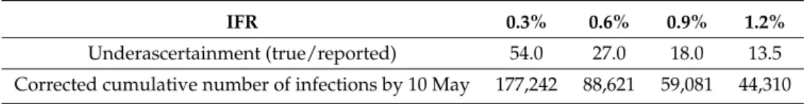
The CFR mentioned in the previous subsection is still not the true value of the fraction of fatal outcomes of all infections, as there is another source of bias, but this time leading to overestimation:

the underascertainment of cases. This is a substantial issue now as a—precisely not yet known, but epidemiologically significant—fraction of the COVID-19 cases are asymptomatic or mildly symptomatic. Since in many countries testing was extended to contacts (and in a few instances, even random sampling was carried out), the confirmed cases include some asymptomatic cases as well.

However, the value of the estimated (corrected) IFR can also be used to estimate the ascertainment rate: by assuming that the IFR in reality takes a benchmark value (one derived from large-sample, well-designed studies accounting for underascertainment or sero-epidemiological surveys) and—crucially—assuming that the difference of the actual estimated IFR from that value is purely due to underascertainment. Then, the ascertainment rate can be obtained by simply dividing the assumed true value of the IFR with the actual estimated CFR [36]. Note that this might be a strong assumption, as it rules out that there is a real difference in the country’s IFR from the benchmark value; in particular, it rules out different virulence of the pathogen, different age- and comorbidity-composition in the country and different effect of the healthcare system on survival.

2.3. Transmission Model

Mathematical models have been developed to better understand the global spread [37] and the transmission dynamics of COVID-19 for many countries, including Australia [38], France [39], Germany [40], UK [41], and the USA [42,43]. Such models have been used to project the progress of the outbreak and to estimate the impact of control measures on reducing disease burden. The two most common approaches are compartmental models formulated as systems of ordinary differential equations, and agent based models used to generate an ensemble of stochastic simulations for possible outcomes.

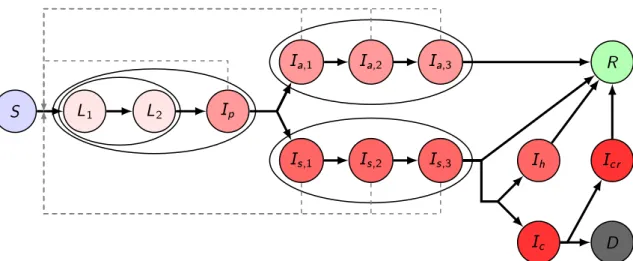
Here, we establish a compartmental population model, adjusted to the specific characteristics of COVID-19, considering the following compartments. We denote bySthe susceptibles, i.e., those who can be infected by the disease. Latents (L) are those who have already contracted the disease but do not show symptoms and are not infectious yet. In accordance with studies indicating that viral shedding peaks before the onset of symptoms [44], in our model, we have introduced the presymptomatic infected compartment I_p for those who do not have symptoms, but who already are capable of transmitting the disease to susceptibles. We divided the latent period into two compartmentsL₁and L₂, thus, together with I_p, the incubation period follows a hypoexponential distribution, having a shape matching empirical observations [45,46]. Since a large fraction of infected shows only mild or no symptoms, after the incubation period, we differentiate these individuals from those with symptoms.

We assume a gamma-distributed infectious period with Erlang parameterm=3, similar to the SARS study [47], hence, we have three classes for both asymptomatic and symptomatic infectious individuals (I_a,1,I_a,2,I_a,3andI_s,1,I_s,2,I_s,3, respectively). Individuals from theI_a,3compartment will all recover and hence proceed to the recovered classR. Immunity is assumed for those who have recovered from the disease, at least for the time scale of this modeling. Individuals fromI_s,3may either recover without

requiring hospital treatment (and thus move toR) or become hospitalized. It is of crucial importance to project the number of hospital beds and intensive care unit (ICU) beds needed; thus, in the model, we further differentiate symptomatically infected individuals who need hospital care and critical care, denoted byI_handI_c, respectively. We operate with the assumption that the healthcare system will not be overwhelmed, and thus disease-induced death is only considered from critical care that fits with the data obtained from NPHC. Hence, individuals fromI_hwill proceed toRafter recovery. Those from I_cwith fatal outcome transit to theDcompartment. Those who are out of ICU and on the path to recovery are collected into theI_cr, from where they eventually recover and move to theRclass.

To take into account the different characteristics of the disease in various age groups, we stratified the Hungarian population into seven groups, corresponding to the available choices in the Hungarian online questionnaire for the assessment of changes in the number of contacts following the lockdown [48]. The compartments listed above corresponding to the different age groups are denoted by an upper indexi∈1, . . . , 7. Accordingly, all of our parameters can be calibrated age-specifically.

The transmission rates from age groupkto age groupiare denoted byβ^(k,i)_j , withj∈ {p,a,s}, where the three subscriptsp,a,sstand for presymptomatic, asymptomatic, and symptomatic infected, respectively. The parameters described in the following all have an upper indexi which stands for the corresponding age group. A fractionpⁱof exposed people will not show symptoms during his/her infection, while (1−pⁱ) will develop symptoms. The average length of the incubation period is (αⁱ_L,1)⁻¹+ (αⁱ_L,2)⁻¹+ (αⁱ_p)⁻¹ days, with the transition rates αⁱ_L,1,αⁱ_L,2,αⁱ_p, respectively.

Similarly, the average infectious period of asymptomatic and symptomatic infected individuals are (γⁱ_a,1)⁻¹+ (γ_a,2ⁱ )⁻¹+ (γⁱ_a,3)⁻¹, and(γⁱ_s,1)⁻¹+ (γⁱ_s,2)⁻¹+ (γⁱ_s,3)⁻¹, with the corresponding transition rates, respectively. A fractionhⁱof the infectious compartmentI_s,3ⁱ will be hospitalized, the remaining fraction 1−hⁱwill recover without hospital care. Out of those who need hospitalization, a fraction ξⁱ needs intensive care. For the hospitalized classes I_hⁱ, I_cⁱ, I_crⁱ , the average time spent in these compartments is given as(γ_hⁱ)⁻¹,(γⁱ_c)⁻¹and(γ_crⁱ )⁻¹, respectively. A fractionµⁱ of those leaving theI_cⁱ compartment will die due to the disease, while the remaining fraction will proceed to theI_crⁱ class. The transmission dynamics of our model for one age group is illustrated in Figure1.

S L

L

I

I

I

I

I

I

I

R

I

I

D I

Figure 1.Transmission diagram. Different shades of red denote infected compartments. A darker shade corresponds to a more severe state of the disease: those in compartments with the lightest shade do not transmit the disease, those in compartments with the darkest shade are in critical status. Black solid arrows denote the possible ways of transition from one compartment to another. Gray dashed arrows show possible ways of infection. Compartments being grouped together in ellipses stand for different stages of the same status.

The governing system of differential Equation (1) of our model can be found in Section2.3.1.

The model parameters with references are detailed in Section2.3.2. A further important component of our model is the contact matrix, describing social mixing between the age groups, which can be found

in Section2.3.3. The elements of the contact matrix are included via the different transmission terms β^(k,i)_j . Reproduction numbers are calculated using the next generation matrix method in Section2.3.4.

We discuss the application and, then, some limitations of this model in Sections 2.3.5 and 2.3.6, respectively. The codes were implemented in Wolfram Mathematica and are available at [49].

2.3.1. The Governing Equations of the Transmission Model

The governing equations of the transmission model described in Section2.3take the form

Sⁱ⁰(t) = − ^S

i(t) Nⁱ(t)

∑

k∈{1,...,7}



β^(k,i)p I_p^k(t) +

∑

j∈{a,s}×{1,2,3}

β^(k,i)_j I_j^k(t)



,

Lⁱ₁⁰(t) = ^S

i(t) Nⁱ(t)

∑

k∈{1,...,7}



β^(k,i)_p I_p^k(t) +

∑

j∈{a,s}×{1,2,3}

β^(k,i)_j I_j^k(t)



−αⁱ_L,1Lⁱ₁(t), Lⁱ₂⁰(t) =αⁱ_L,1L₁ⁱ(t)−αⁱ_L,2Lⁱ₂(t),

I_pⁱ⁰(t) =αⁱ_L,2L₂ⁱ(t)−αⁱ_pI_pⁱ(t), I_a,1^{i 0}(t) =pⁱαⁱ_pI_pⁱ(t)−γⁱ_a,1I_a,1ⁱ (t), I_a,2^{i 0}(t) =γⁱ_a,1I_a,1ⁱ (t)−γⁱ_a,2I_a,2ⁱ (t), I_a,3^{i 0}(t) =γⁱ_a,2I_a,2ⁱ (t)−γⁱ_a,3I_a,3ⁱ (t), I_s,1^{i 0}(t) = (1−pⁱ)αⁱ_pI_pⁱ(t)−γ_s,1ⁱ I_s,1ⁱ (t), I_s,2^{i 0}(t) =γⁱ_s,1I_s,1ⁱ (t)−γ_s,2ⁱ I_s,2ⁱ (t),

I_s,3ⁱ (t) =γⁱ_s,2I_s,2ⁱ (t)−γ_s,3ⁱ I_s,3ⁱ (t), I_hⁱ⁰(t) =hⁱ(1−ξⁱ)γⁱ_s,3I_s,3ⁱ (t)−γⁱ_hI_hⁱ(t),

I_cⁱ⁰(t) =hⁱξⁱγ_s,3ⁱ I_s,3ⁱ (t)−γ_cⁱI_cⁱ(t), I_cr^{i 0}(t) = (1−µⁱ)γⁱ_cI_cⁱ(t)−γⁱ_crI_crⁱ (t),

Rⁱ⁰(t) =γⁱ_a,3I_a,3ⁱ (t) + (1−hⁱ)γ_s,3ⁱ I_s,3ⁱ (t) +γ_hⁱI_hⁱ(t) +γⁱ_crI_crⁱ (t), Dⁱ⁰(t) =µⁱγ_cⁱI_cⁱ(t),

(1)

where the indexi∈ {1, . . . , 7}represents the corresponding age group.

Next, we add the spatial locations of the population to the previous model. The population is divided into patches, where each patch represents a separate geographic region. Within each region, we use the same compartmental model (but possibly with different parameters), and we also include spatial movement of individuals between the patches. The governing equations of such a metapopulation model, wherep₁∈ {1, 2, . . . , #patches}are

Sⁱ_p1⁰(t) = − ^S

pi₁(t) N_pⁱ₁(t)

∑

k∈{1,...,7}



β^(k,i)p₁,pI_p^k_1,p(t) +

∑

j∈{a,s}×{1,2,3}

β^(k,i)_p

1,jI_p^k_1,j(t)





+

#patches p₂=1,p

∑

tⁱ_p2,p1Sⁱ_p2−tⁱ_p1,p2Sⁱ_p1 ,

L_pⁱ_1,1⁰(t) = ^S

ip₁(t) N_pⁱ₁(t)

∑

k∈{1,...,7}



β^(k,i)_p1,pI_p^k_1,p(t) +

∑

j∈{a,s}×{1,2,3}

β^(k,i)_p

1,jI_p^k_1,j(t)



−αⁱ_p1,L,1Lⁱ_p1,1(t) +

#patches p₂=1,p

∑

tⁱ_p2,p1Lⁱ_p2,1−tⁱ_p1,p2Lⁱ_p1,1 ,

L_pⁱ_1,2⁰(t) =αⁱ_p1,L,1Lⁱ_p1,1(t)−αⁱ_p1,L,2Lⁱ_p1,2(t) +

#patches p₂=1,p

∑

tⁱ_p2,p1Lⁱ_p2,2−tⁱ_p1,p2Lⁱ_p1,2 ,

I_pⁱ_1,p⁰(t) =αⁱ_p1,L,2Lⁱ_p1,2(t)−αⁱ_p1,pI_pⁱ_1,p(t) +

#patches p₂=1,p

∑

tⁱ_p2,p1I_pⁱ_2,p−tⁱ_p1,p2I_pⁱ_1,p ,

I_pⁱ_1,a,1⁰(t) =pⁱ_p1αⁱ_p1,pI_pⁱ_1,p(t)−γⁱ_p1,a,1I_pⁱ_1,a,1(t) +

#patches p₂=1,p

∑

tⁱ_p2,p1I_pⁱ_2,a,1−tⁱ_p1,p2I_pⁱ_1,a,1 ,

I_pⁱ_1,a,2⁰(t) =γ_pⁱ_1,a,1I_pⁱ_1,a,1(t)−γⁱ_p1,a,2I_pⁱ_1,a,2(t) +

#patches p₂=1,p

∑

tⁱ_p2,p1I_pⁱ_2,a,2−t_pⁱ_1,p2I_pⁱ_1,a,2 ,

I_pⁱ_1,a,3⁰(t) =γ_pⁱ_1,a,2I_pⁱ_1,a,2(t)−γⁱ_p1,a,3I_pⁱ_1,a,3(t) +

#patches p₂=1,p

∑

tⁱ_p2,p1I_pⁱ_2,a,3−t_pⁱ_1,p2I_pⁱ_1,a,3 ,

I_pⁱ_1,s,1⁰(t) = (1−pⁱ_p1)αⁱ_p1,pI_pⁱ_1,p(t)−γ_pⁱ_1,s,1I_pⁱ_1,s,1(t) +

#patches p₂=1,p

∑

tⁱ_p2,p1I_pⁱ_2,s,1−tⁱ_p1,p2I_pⁱ_1,s,1 ,

I_pⁱ_1,s,2⁰(t) =γ_pⁱ_1,s,1I_pⁱ_1,s,1(t)−γⁱ_p1,s,2I_pⁱ_1,s,2(t) +

#patches p₂=1,p

∑

tⁱ_p2,p1I_pⁱ_2,s,2−tⁱ_p1,p2I_pⁱ_1,s,2 ,

I_pⁱ_1,s,3(t) =γ_pⁱ_1,s,2I_pⁱ_1,s,2(t)−γⁱ_p1,s,3I_pⁱ_1,s,3(t) +

#patches p₂=1,p

∑

tⁱ_p2,p1I_pⁱ_2,s,3−tⁱ_p1,p2I_pⁱ_1,s,3 , I_pⁱ_1,h⁰(_t) =_hⁱ_p

1(₁−ξⁱ_p1)γ_pⁱ_1,s,3I_pⁱ_1,s,3(_t)−γ_pⁱ

1,hI_pⁱ_1,h(_t)_, I_pⁱ_1,c⁰(t) =hⁱ_p1ξⁱ_p1γⁱ_p1,s,3I_pⁱ_1,s,3(t)−γⁱ_p1,cI_pⁱ_1,c(t), I_pⁱ_1,cr⁰(t) = (₁−µⁱ_p1)γⁱ_p1,cI_pⁱ_1,c(t)−γⁱ_p1,crI_pⁱ_1,cr(t)_,

Rⁱ_p1⁰(_t) =γ_pⁱ_1,a,3I_pⁱ_1,a,3(_t) + (₁−hⁱ_p1)γⁱ_p1,s,3I_pⁱ_1,s,3(_t) +γ_pⁱ

1,hI_pⁱ_1,h(_t) +γⁱ_p1,crI_pⁱ_1,cr(_t) +

#patches p₂=1,p

∑

tⁱ_p2,p1Rⁱ_p2−tⁱ_p1,p2Rⁱ_p1 , Dⁱ_p1⁰(t) =µⁱ_p1γ_pⁱ_1,cI_pⁱ_1,c(t).

(2)

2.3.2. Model Parameters

We have chosen our model parameters based on comprehensive literature review and present them here, except the transmission rates β^(k,i)_{s,_} which are left for Section2.3.4. For the incubation period, we assume hypoexponential (generalized Erlang) distribution with parameters (1.6, 1.6, 2).

This way, the average incubation period is 5.2 days: the same length and very similar shape of the

probability distribution function was estimated in [45], and this distribution has the observed concavity properties as well (see [46]). In addition, this estimation is consistent with [34], and such values have been used in [38,39,41,42]. The first 3.2 days are the latent period [38] and the past two days are the presymptomatic period [38], when transmission is already possible with similar rate as at symptom onset [44]. Therefore, we use the same transmission rates for the presymptomatic and symptomatic infectious periods. For the transmission rate of asymptomatic infected individuals, we use a reduction factor 0.5 [39,42,43].

For the length of infectious periods (both symptomatic and asymptomatic), we assume a gamma distribution with Erlang parameter 3 (coherent with the SARS study [47]), and an average length 3 days of infectivity. Although full recovery and viral shedding may take much longer, the infectiousness throughout the course of infection is mostly concentrated to this period [44,50]. The choice of 3 days is also justified by [44,51], who estimated that around 40% of transmissions occur during the presymptomatic period, and it is also within the range of infectious periods used by [39,42].

The average stay in hospital is assumed to be 10 days, in accordance with the seven days median reported in [52] using over 16,000 patients’ data in the UK. Similarly, the average duration of critical care is assumed to be 10 days, in accordance with the Intensive Care National Audit & Research Center (ICNARC) report [53]. Very similar numbers were reported in the US [54], and were used in other modeling studies [38,41,42]. For those who recover from intensive care, we assumed a 14-day hospitalized rehabilitation period.

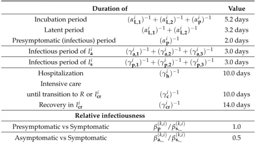
The periods above associated with the average time an individual spends in each compartment over the course of the infection are age-independent and summarized in Table1.

Table 1.Age-independent epidemiological parameters of COVID-19. Assumed to be valid for all age groups. References and explanations are in Section2.3.2.

Duration of Value

Incubation period (αⁱ_L,1)⁻¹+ (αⁱ_L,2)⁻¹+ (αⁱ_p)⁻¹ 5.2 days Latent period (αⁱ_L,1)⁻¹+ (αⁱ_L,2)⁻¹ 3.2 days Presymptomatic (infectious) period (αⁱ_p)⁻¹ 2.0 days Infectious period ofI_aⁱ (γⁱ_a,1)⁻¹+ (γⁱ_a,2)⁻¹+ (γⁱ_a,3)⁻¹ 3.0 days Infectious period ofI_sⁱ (γⁱ_p,1)⁻¹+ (γⁱ_p,2)⁻¹+ (γ_p,3ⁱ )⁻¹ 3.0 days

Hospitalization (γⁱ_h)⁻¹ 10.0 days

Intensive care

until transition toRorI_crⁱ (_γⁱ_c)⁻¹ 10.0 days

Recovery inI_crⁱ (γⁱ_cr)⁻¹ 14.0 days

Relative infectiousness

Presymptomatic vs Symptomatic β^(k,i)_p /β^(k,i)_{s,_} 1.0 Asymptomatic vs Symptomatic β^(k,i)a,_ /β^(k,i)s,_ 0.5

Next, we discuss the age-specific parameters, which are mostly related to the outcome of infections.

We stratified the population into the following seven age groups: 0–4, 5–14, 15–29, 30–59, 60–69, 70–79, 80+years old. Using the data from the Hungarian Central Statistical Office (KSH), we obtain the division shown in Table2.

Table 2.Age groups of the Hungarian population.

Age group 0–4 5–14 15–29 30–59 60–69 70–79 80–

Population 468,605 953,134 1,678,211 4,087,976 1,312,208 839,589 433,033

According to [55], a fraction 0.8 of infected children (under 18 years old) are asymptomatic or mild cases. This value was used in [42] as well. We set the probabilities of the infection following mild or asymptomatic course in an individual according to Weitz et al. [43].

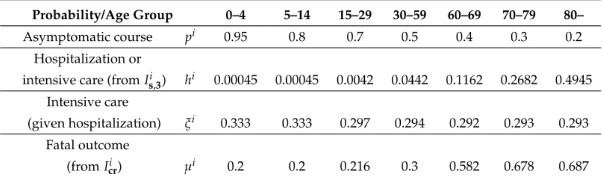
The probabilities of hospitalization given infectionhⁱand of requiring intensive care in additionξⁱ are based on the work of Moss et al. [38]. The ratios of fatal outcomesµⁱare derived from the ICNARC report [53] comprising 6720 ICU case reports from UK. All these age-dependent parameters are listed in Table3.

Table 3. Age-dependent epidemiological parameters of COVID-19.

Probability/Age Group 0–4 5–14 15–29 30–59 60–69 70–79 80–

Asymptomatic course pⁱ 0.95 0.8 0.7 0.5 0.4 0.3 0.2

Hospitalization or

intensive care (fromI_s,3ⁱ ) hⁱ 0.00045 0.00045 0.0042 0.0442 0.1162 0.2682 0.4945 Intensive care

(given hospitalization) ξⁱ 0.333 0.333 0.297 0.294 0.292 0.293 0.293 Fatal outcome

(fromI_crⁱ ) µⁱ 0.2 0.2 0.216 0.3 0.582 0.678 0.687

2.3.3. Contact Matrix

For creating our contact matrixMcont, we have utilized the work by Prem, Cook, and Jit [56], where the estimated matrices are written for 16 age groups, namely 0–4, 5–9,. . . , 70–74, 75+. As we have divided the Hungarian population into seven age groups, see Table2, we aggregated the higher resolution data. First, we derived a symmetric matrixM^totalwith elements

m^total_i,j = ^mi,jpi+mj,ipj

2 ,

whereM= [mi,j]is the original contact matrix and[pi]is the age distribution of Hungary for the same age groups as in [56]. Thus,M^totalcontains the total number of contacts among age groups in its upper triangular part (with values relative to the contact pattern inM). The total number of contacts, w.r.t. the age distribution used in our work, is then obtained by summing up the corresponding elements of this matrix of size 16×16 resulting inM^total_contof size 7×7. Finally, dividing element-wise each column of M^total_contby the aforementioned population vector given in2yields the following 7×7 contact matrix:

Mcont=























2.85266 1.01297 0.979001 3.66453 0.759418 0.250632 0.153184 0.498022 5.54587 1.36396 4.67031 0.715084 0.485708 0.255501 0.273365 0.774654 6.17901 6.44003 0.594565 0.283886 0.13613 0.420065 1.08891 2.64379 5.45488 0.905271 0.411717 0.185912 0.271197 0.519408 0.760402 2.82023 1.66402 0.585505 0.162196 0.139887 0.551395 0.567445 2.00466 0.915096 0.736195 0.144611 0.165767 0.562374 0.527571 1.75507 0.491497 0.28038 0.55053





















 .

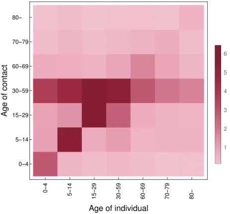
For more insight, we include its heatmap in Figure2. Additional technical details are to be found in our source code available at [49].

0-4 5-14 15-29 30-59 60-69 70-79 80- 0-4

5-14 15-29 30-59 60-69 70-79 80-

Age of individual

Ageofcontact

1 2 3 4 5 6

Figure 2.Heatmap of the contact matrixMcont. The image is rotated w.r.t. howMcontis indexed: the (1, 1)element is in the bottom-left corner.

2.3.4. Transmission Rates and the Next Generation Matrix

Recall that we have assumed presymptomatic patients, which are members of classesI_pⁱ, to be as infectious as symptomatic patients. In addition, patients with no or mild symptoms (those inI_aⁱ) possess a transmission coefficient half of the baseline.

Thus, our task is to give reasonable estimates for the ratesβ^(k,i)s,_ corresponding to the transmission rate of the symptomatic individuals from age groupkto groupi. To that end, we follow the terminology and techniques of [57] to compute the Next Generation Matrix (NGM) and the baseline transmission rateβ₀. Finally, the desired coefficients are obtained by taking into account the relative contact rates between age groups via the contact matrix presented in Section2.3.3. We note that the probabilities pⁱhave a special role during NGM computations as their effect is what ultimately specializes the resulting transmission rate matrix for COVID-19.

First, let us consider the infectious subsystem of (1), namely, equations describingLⁱ₁⁰(t),Lⁱ₂⁰(t), I_pⁱ⁰(t), and I_jⁱ⁰(t) withj ∈ {a,s} × {1, 2, 3},i ∈ {1, . . . , 7}. Linearizing this w.r.t. the disease free equilibrium yields the linearized infectious subsystem:

X⁰(t) = (T+_Σ)·X(t),

where the matricesTandΣare referred to as thetransmission partandtransitional part, respectively;

the state is described by X(t) =transpose h

{Lⁱ₁(t) Lⁱ₂(t) I_pⁱ(t) {I_a,nⁱ (t)}_n=1...3 {I_s,nⁱ (t)}_n=1...3}_i=1...7ⁱ .

Recall that the transmission matrixThas the form

T=























T1

0 . . . (2^ndrow) . . . 0

... ... ...

0 . . . (8^throw) . . . 0 T2

... ... ...





















 ,

whereTi=T1,i T2,i T3,i T4,i T5,i T6,i T7,i with

T_k,i=^h_{0 0 β}^(k,i)_{p β}^(k,i)_{a,1 β}^(k,i)_{a,2 β}^(k,i)_{a,3 β}^(k,i)_{s,1 β}^(k,i)_{s,2 β}^(k,i)_s,3 ⁱ. On the other hand, the transitional matrixΣis block diagonal with blocks

Σi =

































−αⁱ_L,1 0 0 0 0 0 0 0 0

αⁱ_L,1 −αⁱ_L,2 0 0 0 0 0 0 0

0 αⁱ_L,2 −αⁱ_p 0 0 0 0 0 0

0 0 pⁱαⁱ_p −γ_a,1ⁱ 0 0 0 0 0

0 0 0 γⁱ_a,1 −γⁱ_a,2 0 0 0 0

0 0 0 0 γⁱ_a,2 −γⁱ_a,3 0 0 0

0 0 (1−pⁱ)αⁱ_p 0 0 0 −γ_s,1ⁱ 0 0

0 0 0 0 0 0 γⁱ_s,1 −γ_s,2ⁱ 0

0 0 0 0 0 0 0 γⁱ_s,2 −γ_s,3ⁱ

































fori=1, . . . , 7.

Then, the NGM with large domain is given by K_L =−_TΣ⁻¹ and the NGM

K=E KLtranspose(E)

follows with the, again, block diagonalEwithE_i= [1 0 0 0 0 0 0 0 0]. The baseline transmission rateβ₀may be factored out fromKasβ^(k,i)_p =β^(k,i)_s =β₀·(Mcont)_k,iandβ^(k,i)_a = ¹₂β^(k,i)_s =β₀· ^(Mcont₂ ^)k,i. Hence,K=β₀·K, where ˆ^ˆ Kmay be readily constructed and we can compute its spectral radiusρ(K^ˆ). Then, we obtain the baseline transmission rate using the assumed basic reproduction numberR₀as

β0·ρ(K^ˆ) =R₀,

which isβ₀≈0.0462 forR₀=2.2. Finally, the transmission ratesβ^(k,i)_s are computed via the contact matrixMcontas

β^(k,i)s

k,i=β0Mcont=























0.131931 0.0468484 0.0452773 0.169479 0.035122 0.0115914 0.00708453 0.0230328 0.256488 0.0630811 0.215995 0.0330716 0.0224633 0.0118165 0.0126427 0.0358266 0.28577 0.297842 0.0274977 0.0131293 0.00629581 0.0194274 0.0503605 0.122271 0.25228 0.0418674 0.0190413 0.00859815 0.0125425 0.0240218 0.0351675 0.130431 0.0769585 0.0270787 0.00750132 0.00646957 0.0255012 0.0262435 0.0927126 0.0423218 0.0340479 0.00668804 0.00766648 0.026009 0.0243994 0.0811694 0.022731 0.0129672 0.0254612





















 ,

again, forR₀=2.2. For other scenarios, the final steps are altered to align with the desired reproduction number R, resulting in an appropriate βand then the scaled transmission rates β^(k,i)_s . We omit presenting all transmission matrices but give the computed baseline transmission rates in Table4.

Table 4.Baseline transmission rates from NGM computation.

R 1.0 1.1 1.32 1.65 2.2 β 0.0210 0.0231 0.0277 0.0347 0.0462

2.3.5. Scenarios

We use the compartmental model described above to explore possible future scenarios, assuming widespread transmission in the population. In particular, we investigate the disease dynamics when different levels of general reductions of transmission, compared to the baseline, are in place.

By manipulating the contact matrix, we investigate the effect of age-specific interventions, such as school closures and special measures aimed to protect the elderly.

Seasonality of respiratory viruses can be attributed to a combination of factors, including the survival of the virus in different environmental conditions, changes in contact patterns (such as school holidays), less time spent in closed spaces where the highest number of transmissive contacts are made, and potentially seasonal changes in the health conditions of the population as well. To express this behavior, we define a time-dependent parameter

ω(c,t) =0.5·c·cos 2πt

366

+ (1−0.5·c) (3)

by which we scale the transmission rate β. Parameter c denotes the magnitude of the effect of seasonality on the number of contacts. Using such a time-dependent transmission rate, we compare possible disease dynamics generated by the interplay of control measures with different degrees of seasonal behavior.

Spatial heterogeneity is also considered using our patch model, where the country is divided into distinct geographic regions (patches). The transmission dynamics is described within each patch by our compartmental model (but potentially with different parameters and age group composition), and individuals may move between those patches. For obvious reasons, individuals in compartments I_hⁱ,I_cⁱ,I_crⁱ and Dⁱ do not travel. Lettravel_p,q denote the number of travels from patch p to patchq.

To derive travel ratest_p,qfor each age groupi, we divide the number of travels with the population of the appropriate patch

tⁱ_p,q= ^travelp,q N_p(t) ^.

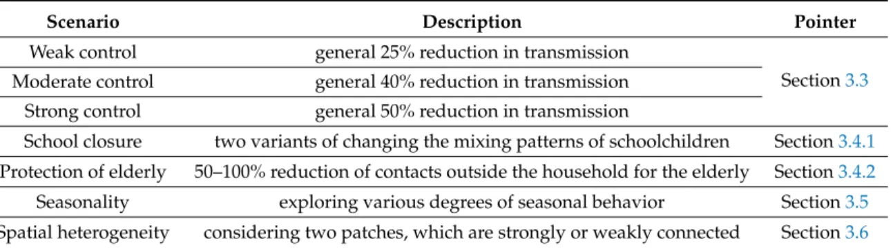
Numerical simulations for such situations show the differences in the transmission dynamics, healthcare demand, mortality, and overall disease burden. These scenarios are summarized in Table5.

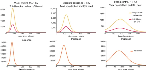
Table 5.Scenarios.

Scenario Description Pointer

Weak control general 25% reduction in transmission

Section3.3 Moderate control general 40% reduction in transmission

Strong control general 50% reduction in transmission

School closure two variants of changing the mixing patterns of schoolchildren Section3.4.1 Protection of elderly 50–100% reduction of contacts outside the household for the elderly Section3.4.2 Seasonality exploring various degrees of seasonal behavior Section3.5 Spatial heterogeneity considering two patches, which are strongly or weakly connected Section3.6