Spin Chain Overlaps and the Twisted Yangian

Spin Chain Overlaps and the Twisted Yangian

Marius de Leeuw¹, Tamás Gombor², Charlotte Kristjansen³, Georgios Linardopoulos⁴ and Balázs Pozsgay⁵

1School of Mathematics & Hamilton Mathematics Institute Trinity College Dublin

2Wigner Research Centre for Physics

3Niels Bohr Institute University of Copenhagen

4Institute of Nuclear and Particle Physics, N.C.S.R., "Demokritos"

5MTA-BME Quantum Dynamics and Correlations Research Group, Department of Theoretical Physics,

Budapest University of Technology and Economics

mdeleeuw@maths.tcd.ie, gombor.tamas@wigner.mta.hu, kristjan@nbi.dk, glinard@inp.demokritos.gr, pozsi@eik.bme.hu

Abstract

Using considerations based on the thermodynamical Bethe ansatz as well representation theory of twisted Yangians we derive an exact expression for the overlaps between the Bethe eigenstates of theSO(6) spin chain and matrix product states built from matrices whose commutators generate an irreducible representation ofso(5). The latter play the role of boundary states in a domain wall version ofN = 4 SYM theory which has non-vanishing, SO(5) symmetric vacuum expectation values on one side of a co-dimension one wall. This theory, which constitutes a defect CFT, is known to be dual to a D3-D7 probe brane system.

We likewise show that the same methodology makes it possible to prove an overlap formula, earlier presented without proof, which is of relevance for the similar D3-D5 probe brane system.

Keywords: Super-Yang-Mills Theory; Defect CFTs; One-point functions; Twisted Yangians, D3-D7 probe-brane model; Spin chain overlaps

Contents

1 Introduction and summary 2

2 One-point functions in AdS/dCFT 4

2.1 The SO(5) symmetric domain wall theory 4

2.2 One point functions from matrix product states 5

2.3 Exact results for one-point functions 7

2.4 Strategy of derivation 8

3 Integrability tools for overlaps 9

3.1 The integrable boundary reflection matrix 9

3.2 Quantum transfer matrices and the fusion hierarchy 11

3.3 TBA and overlaps 14

4 Application of the TBA 17

4.1 Overlaps with symmetry class (SU(3), SO(3)) 17

4.2 An overlap with symmetry class (SO(6), SO(5)) 19

4.3 An overlap with symmetry class (SO(6), SO(3)×SO(3)) 20

5 The twisted Yangian 21

5.1 Approach 21

5.2 Definitions and preliminaries 22

5.3 (SU(3),SO(3)) case 27

5.4 (SO(6),SO(5)) case 32

6 Conclusion and outlook 33

A Limiting formulas for the overlaps 35

B Calculations with the twisted Yangian Y⁺(3) 35

B.1 Oddk= 2s+ 1 36

B.2 Evenk= 2s+ 1 39

C Calculations with the twisted Yangian X(so₆,so₅) 42

1 Introduction and summary

A surprisingly fruitful cross-fertilization between holography and statistical physics has taken place in recent years due to a common interest in overlaps between Bethe eigenstates of integrable systems and states which are not easily expressible in terms of eigenstates.

In statistical physics the latter type of state typically constitutes the initial state in a quantum quench of an integrable system and the overlaps are key to investigating the time development after the quench, see f.inst. [1–8]. In holography the typical state of interest is a so-called matrix product state which encodes information about the vacuum of the holographic system and the overlaps give the expectation value of the theory’s operators in the vacuum state [9–14].

From the point of view of holography, systems which are amenable to an analysis of this type are domain wall versions of N = 4 SYM theory where the vacuum is different on the two sides of a co-dimension one wall. More precisely, the vacua on the two sides of the wall differ by some of the scalar fields taking non-zero vacuum expectation values (vevs) on one side, say for x₃ >0. These field theories constitute defect conformal field theories (dCFTs) and are dual to probe brane systems with configurations of background gauge fields which lead to non-trivial flux or instanton number [15–21]. There are essentially three such systems, one being a D3-D5 probe brane system and the two others being D3-D7 probe brane systems, cf. table 1. In dCFT’s one can encounter non-vanishing one-point functions and due to the non-trivial vacuum expectation values this will happen already at tree-level for the set-ups in question. As first pointed out in [9,10] the tree level one point functions of scalar operators forx₃>0 can conveniently be expressed as an overlap between a matrix product state and a Bethe eigenstate of theSO(6) integrable spin chain.

Both from the point of view of statistical physics and from the point of view of holography it is interesting to understand when a certain initial state or a matrix product state is “solvable”, i.e. under what circumstances the various physical quantities associated to the state can be computed exactly. One class of such quantities are the overlaps with the Bethe eigenstates of the system. Based on the experience from a number of concrete studies of overlaps [9–12, 22–25] a proposal for an integrability criterion was put forward in [5]. An initial state or matrix product state was said to be integrable if it was annihilated by all the conserved charges of the integrable system, which were odd under space-time parity.

All the overlaps which were known in closed form at that time were compatible with this definition of integrability. This was in particular true for the dCFT dual to the 1/2 supersymmetric D3-D5 probe brane system with background gauge field flux where a closed expression for all the one-point functions of the scalar sector had been found [13]. When applied to the two non-supersymmetric D3-D7 probe brane set-ups with flux the proposed integrability criterion implied a characterization of one of them as integrable and the other one as non-integrable cf. table1. This led to an apparent puzzle since for none of them a closed expression for the overlaps had been found [12,14].

In the present paper we resolve this apparent puzzle and provide another strong consistency check of the proposed integrability criterion by explicitly deriving a closed formula for the overlap giving the scalar one-point functions of theSO(5) symmetric D3-D7 probe brane set-up with non-vanishing instanton number. Our proof combines analyticity considerations related to the thermodynamical Bethe ansatz with representation theory of twisted Yangians. We also show that a similar approach can be used to prove the overlap formula for the D3-D5 probe brane system, earlier presented without proof. For simplicity we carry out the proof only for an SU(3) sub-sector in this case.

D3-D5 D3-D7 D3-D7

Supersymmetry 1/2-BPS None None

Brane geometry AdS₄× S² AdS₄×S² × S² AdS₄× S⁴

|MPSi Integrable Non-integrable Integrable

Closed overlap formula Yes No Yes (this work)

Table 1. The dCFT versions ofN = 4 SYM theory with non-vanishing vevs and their dual string theory configurations. The discussion of the integrability properties of the corresponding matrix product states can be found in [13, 14] and the closed expression for the overlap formula for the D3-D5 case appears in [9–11,13] for tree level and in [26] for one-loop.

We start in section 2 by briefly discussing the dCFT withSO(5) symmetric vevs and the matrix product state which is used to calculate its one-point functions. In this section we also present the closed form of the overlap for any scalar operator and for any value of the instanton number. Subsequently, in section3, we introduce some integrability tools that will play an important role for our analysis. In particular, we explain the connection between the overlaps and the Y-system. Based on analyticity considerations for theY-system we then in section4 derive overlap formulas for a set of simple “base” states with respectively SO(3) andSO(5) symmetry. In section5 we review elements of the representation theory of twisted Yangians and use these ideas to relate the base states to the desired matrix product states and in that way derive the desired overlap formulas. Section6 contains our conclusion and outlook. Some technical details are relegated to appendices.

2 One-point functions in AdS/dCFT

2.1 The SO(5) symmetric domain wall theory

We will be considering a domain wall version of N = 4 SYM theory with gauge group U(N) where the theory has a non-trivial vacuum on one side of the wall. More precisely, we consider a co-dimension one wall placed atx₃= 0 and we allow for (some of) the scalar fields of the theory to have non-vanishing classical values for x3 >0. Assuming ψ^cl =A^cl_µ = 0, the classical values for the scalar fields have to fulfil the equation

∇²φ^cl_i =^hφ^cl_j,^hφ^cl_j, φ^cl_i ⁱⁱ, i= 1, . . . ,6. (2.1) By allowing the classical fields to depend on the distance to the defect x3 one can obtain a defect CFT. Anso(5) symmetric solution with such space-time dependence was found

in [16,27]

φ^cl_i (x) = 1

√ 2x3

G_i 0 0 0

!

, i= 1, . . . ,5, φ^cl₆(x) = 0, x3>0, (2.2) where the classical fields are N ×N matrices containing the sub-matricesG_i of dimension dG×dG with

d_G= 1

6(n+ 1)(n+ 2)(n+ 3), n∈Z. (2.3) They can be constructed starting from a four-dimensional representation of the Clifford algebraso(5)

{γ_i, γj}= 2δi,jI4×4, (2.4) and symmetrizing the n-fold tensor product

G_i = 1

2 γ_i⊗1⊗ · · · ⊗1

| {z }

nfactors

+· · ·+ 1⊗ · · · ⊗1⊗γ_isym, (2.5) The commutators of the G_i then generate ad_G-dimensional irreducible representation of so(5). We refer to section5 for a discussion of further properties of the G_i. Forx₃ <0 all fields are considered to be of dimension (N−dG)×(N−dG) with vanishing classical values implying that the gauge group of the field theory is different on the two sides of the wall, namely respectively (broken)U(N) for x3 >0 andU(N−dG) for x3 ≤0¹.

This domain wall solution of N = 4 SYM theory has a string theory dual consisting of a D3-D7 probe brane system where the D7-brane probes have geometry AdS₄ ×S⁴ and a non-trivial instanton bundle on theS⁴ carries instanton number equal todG. The probe is the string theory analogue of the gauge theory wall and the change in gauge group across the wall is reflected ind_G out of theN D3-branes being dissolved into D7-branes as x3 →0+ [31]. The probe brane system is stable in the parameter region

λ

π²(n+ 1)(n+ 3) < 2

7, (2.6)

where λis the ’t Hooft coupling, proportional to the inverse string tension according to the AdS/CFT dictionary.

2.2 One point functions from matrix product states

Due to the restricted amount of symmetries of defect CFTs these theories allow for additional classes of correlation functions compared to ordinary CFTs and their two- and three-point functions are more involved than for ordinary CFTs. We shall normalize our operators

1The consistency of this set-up is confirmed by perturbative calculations. One finds that almost all field excitations forx3 >0 which are outside the (N−dG)×(N−dG) block become infinitely heavy as the wall is approached and have propagators with support only in the regionx3>0 [28]. For a few remaining excitations this is not the case but for these one needs to impose Dirichlet or Neumann boundary conditions at the wall to obtain the gauge symmetryU(N−dG) exactly at the wall [29,30].The few special excitations can be ignored in the large-N limit.

such that the two-point functions take the canonical form of an ordinary CFT far from the defect, i.e.

z3lim→∞hO_i(x+z)O_j(y+z)i= δij

|x−y|^∆i+∆j, (2.7) where the ∆’s are the conformal dimensions of the operators involved. Our main object of interest will be the one-point functions which are restricted to take the following form

hO_∆(x)i= C

x^∆₃ . (2.8)

Due to the non-trivial vevs, one-point functions of operators built from the five scalars φ1, . . . , φ5 will have non-vanishing one-point functions forx3>0 already at tree level. As is well-known [32] the good conformal operators containing only scalar fields can be described at the lowest loop level as the eigenstates of an integrableSO(6) spin chain given by the R-matrix

R(u) =u(u+ 2)I+ (u+ 2)P−uK, (2.9) where P is the permutation operator andKis the trace operator. These eigenstates can in turn be expressed in terms of three sets of Bethe roots{u_i}^N_i=1⁰ ,{v_j}^N_j=1⁺,{w_k}^N_k=1⁻which fulfil a set of algebraic Bethe equations. The ui’s are the so-called momentum carrying roots. We shall collectively refer to the Bethe roots as u and the corresponding eigenstate as |ui. Determining the one-point function of a conformal operator at tree level amounts to inserting the vevs from eqn. (2.2) into the Bethe wave function describing the operator, a procedure which can conveniently be formulated as calculating the overlap of the Bethe eigenstate with a matrix product state (MPS) of bond dimension dG, i.e. [9,10]

C= 8π² λ

!^L

2

L⁻¹² C_n, C_n= hu|MPS_ni hu|ui¹²

, (2.10)

where

|MPS_ni=^X

~i

tr[Gi1. . . GiL]|φ_i1. . . φiLi, (2.11) with n referring to the dimension of the representation for the vevs via eqn. (2.3). In practice it is more convenient to work with complex combinations of the scalar fields defined as follows

X =φ1+iφ2, Y =φ3+iφ4, Z =φ5+iφ6, (2.12) X¯ =φ₁−iφ₂, Y¯ =φ₃−iφ₄, Z¯=φ₅−iφ₆. (2.13) The dictionary between Bethe eigenstates |ui and operators built from complex fields can be found for instance in [32].

2.3 Exact results for one-point functions

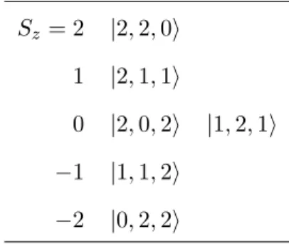
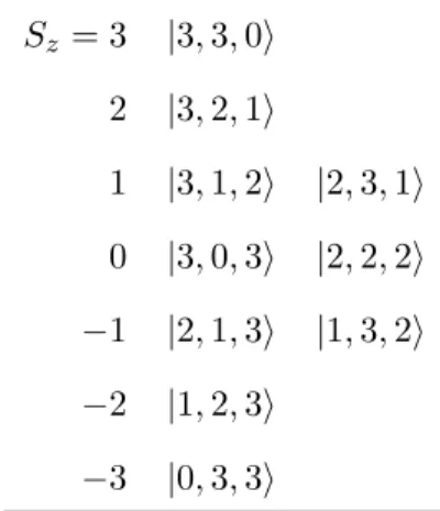
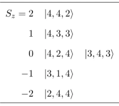
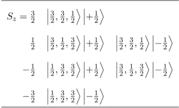
Exploiting the symmetry properties of theG-matrices one can derive the following selection rule that needs to be fulfilled in order for an operator to have a non-vanishing one-point function [12]

(L, N₀, N₊, N−) = (L, N₀, N₀/2, N₀/2), N₀ even, (2.14) where L is the number of fields of the operator. Furthermore, it was shown in [13] that the matrix product state (2.11) is annihilated by all the odd charges of the integrable SO(6) spin chain and hence obeys the integrability criterion proposed in [5]. The fact that the matrix product state is annihilated by all the odd charges gives rise to a number of constraints on the possible sets of Bethe roots. First, the momentum carrying roots have to come in pairs with opposite sign of the momenta or rapidities. The same is the case for the other two types of roots if their number N₀/2 is even. IfN₀/2 is odd the paired roots must be supplemented by a single additional root at zero [12,13]. In the remaining part of this paper we will show that in accordance with the integrability criterion being fulfilled there does exist a closed formula for the one-point functions in the present case. The formula is expressed in terms of objects well known from the study of integrable spin chains, namely the Gaudin determinant [33,34] which gives the norm of a Bethe eigenstate and three types of Baxter polynomials corresponding to the three types of Bethe roots,

Q0(a) =

N0

Y

i=1

(ia−ui), Q+(a) =

N0/2

Y

j=1

(ia−vj), Q−(a) =

N0/2

Y

k=1

(ia−w_k). (2.15) The overlap formula reads

hu|MPS_ni²

hu|ui = Λ²_n· Q0(0)Q0

₁

2

Q¯+(0) ¯Q+

1 2

Q¯−(0) ¯Q−

1 2

·detG₊ detG−

, (2.16)

where the bar on the Q’s signifies that a Bethe root at zero should be excluded from the Baxter polynomial and where detG is the determinant of the Gaudin matrix which for Bethe states with the roots paired as above factors as detG= detG₊detG−.^2,3

The pre-factor Λ_n is a specific transfer matrix eigenvalue, which will be explained later.

For n= 1 which corresponds to the Gi being the Dirac gamma matrices we find for the pre-factor

Λ₁ =1 + (−1)^L Q₀(1)

Q0(0)+ (−1)^N−Q−

3 2

Q−

1 2

+ (−1)^L+N+Q+

3 2

Q₊¹₂

, (2.17)

2As far as we know the first appearance of a finite volume overlap involving this ratio of Gaudin-like determinants was in [35], where a rather general explanation for the ratio was given by focusing on the density of states. The work [35] treated the excited stateg-functions in integrable QFT, which are analogous to the finite volume spin chain overlaps. In spin chains the same structure was found independently in [23].

3For an illustration of the factorization of the Gaudin determinant in a case with nested Bethe ansatz, see [11].

An expression valid for any n∈N can likewise be derived and takes the form Λ_n= 2^L

n 2

X

q=−ⁿ₂

q^L

" _q X

p=−ⁿ₂

Q₀(p−¹₂) Q₀(q−¹₂)

Q−(q)Q−(ⁿ₂ + 1) Q−(p)Q−(p−1)

#" ⁿ₂ X

r=q

Q₀(r+¹₂) Q₀(q+¹₂)

Q₊(q)Q₊(ⁿ₂ + 1) Q₊(r)Q₊(r+ 1)

# . (2.18) IfN₀/2 is even the formula immediately gives the value of Λ_n. If N₀/2 is odd andnis even there can be singularities of the type 0/0 coming from the Baxter polynomials Q+ andQ−

being evaluated at zero. In this case the formula (2.18) still holds but should be understood in a limiting sense so that for instance forn= 2 and N0/2 even we get

Λ₂ = 2^L+1·

"

1 + (−1)^L

2 ·Q₀³₂ Q₀¹₂

+Q−(2)

Q−(0) + (−1)^L·Q+(2) Q+(0)

#

, N0/2 even, (2.19) whereas forn= 2 and N0/2 odd the result reads

Λ₂= 2^L+1·

"

1 + (−1)^L

2 ·Q₀³₂ Q₀¹₂

+Q−(2) Q¯−(0)





Q⁰₀¹₂ Q₀¹₂

−Q⁰₋(1) Q−(1)



+ (2.20)

+ (−1)^L·Q+(2) Q¯₊(0)





Q⁰₀¹₂ Q₀¹₂

−Q⁰₊(1) Q₊(1)





#

, N0/2 odd.

The generalization of this formula to arbitrary values of n can be found in appendixA.

2.4 Strategy of derivation

The overlap formula given by (2.16) and (2.18) has a rather intricate structure with the pre-factor of the determinant term involving a sum over products of Q-functions. Most overlap formulas for which an explicit derivation has been possible until now have only a single product as a pre-factor. This holds for the overlaps of the XXZ spin chain between Bethe eigenstates and general two-site product states [36], including the Néel state, the dimer state and theq-deformed dimer state [22–24]. It also holds for overlaps of the XXX Heisenberg spin chain with matrix product states which are built from the generators of su(2) in the spin-1/2 representation [9]. An exception is the generalization of the latter overlaps to higher representations for which a recursive strategy for the derivation could be pursued [10].

In cases where the pre-factor in the overlap formula consists of a single product the pre-factor can be found by making use of the thermodynamical Bethe ansatz and exploiting certain analyticity properties of the Y-functions [36]. For instance, this method makes it possible to prove an overlap formula, first presented in [11], for theSU(3) spin chain between Bethe eigenstates and certain matrix product states built from Pauli-matrices, as we shall show in section 4.1. However, if the pre-factor is more involved, the method only gives its leading behaviour in the thermodynamical limit.

Currently, there exists a number of more involved overlap formulas which have been presented without proof. One gives the overlap formula of the SU(3) spin chain with matrix product states built from generators ofsu(2) in higher representations and another one gives the overlap formula for the integrable SO(6) spin chain with similar matrix product states [13]. As a side-track of the investigations of the present paper we shall prove the former of these two formulas which we characterize in terms of symmetries as the (SU(3), SO(3)) case. Our main goal, however, is to derive the formula (2.16), for which no proposal existed up to now. This case will correspondingly be denoted as the (SO(6), SO(5)) case.

Our strategy for deriving the overlap formulas is the following. First we compute the overlap for a simple matrix product state built from one or two-site states using the TBA approach. Subsequently we use the representation theory of twisted Yangians to relate the desired more complicated MPS’s to the simple ones, invoking in the process a reflection matrix fulfilling the relevant boundary Yang Baxter equation.

In order to verify intermediate steps in the procedure as well as the final formula we also calculated the desired overlaps numerically. The Bethe states were constructed either by using the appendix E.5 of [37] or by explicitly diagonalizing the Hamiltonian.

The corresponding Bethe roots have been obtained with the “Fast Bethe Solver” program [38–40].⁴ Details of the tests performed can be found in appendixA.

3 Integrability tools for overlaps

In this section we present the main ingredients needed for our derivation of the overlap formula. First, we recall the definition of integrable initial states and explain that this concept is related to the existence of an integrable boundary reflection matrix which can be used to form a double row transfer matrix. Secondly, we review the construction of the so-called fusion hierarchy of the double row transfer matrix as well as the associated Y-functions. Finally, we explain how the Y-functions determine the singularity structure of the overlap formulas via the thermodynamical Bethe ansatz (TBA).

3.1 The integrable boundary reflection matrix

We consider local integrable spin chains, where the local Hilbert space on each site isC^N with someN ≥2. The model has an associated fundamentalR-matrixR(u)∈End(C^N ⊗C^N) which enjoys a symmetry with respect to a Lie group G. In the concrete examples we will focus on G=SU(N) and G=SO(N).

We define the monodromy matrix of a homogeneous spin chain of length Las

T(u) =R_0L(u). . . R₀₂(u)R₀₁(u). (3.1) Here 0 refers to the so-called auxiliary space, and in our examples V0 ≈C^N. The transfer matrix is the trace over the auxiliary space:

t(u) = Tr0T(u). (3.2)

4We would like to thank to C. Marboe and D. Volin for informative discussions and for sharing their code with us.

We also define the space reflected transfer matrix:

¯t(u) = Πt(u)Π = Tr0 R01(u). . . R_0L(u). (3.3) An initial state |Ψi is said to be integrable if the following condition is fulfilled [5,8]

t(u)|Ψi= ¯t(u)|Ψi. (3.4)

We will be interested in a specific type of initial states, namely matrix product states defined by

|Ψ_ωi=

N

X

j1,...,jL=1

tr_a[ω_jL. . . ω_j2ω_j1]|j_L, . . . , j₂, j₁i, (3.5) where the matrices ωj, j = 1, . . . , N act on a further auxiliary space Va. Typically the matrix product state (MPS) is invariant with respect a subgroup G⁰ ⊂ G. In this case we say that the symmetry class of the problem is (G,G⁰). In the cases encountered so far the two Lie groups are a symmetric pair. In [8] it was found that an MPS is integrable in the sense described above if it can be embedded into the framework of the (twisted) Boundary Yang-Baxter relation. We now describe this connection.

Let us consider a rapidity dependent two-site block ψ(u)∈C^N ⊗C^N ⊗End(Va). It is useful to think about ψ(u) as a collection of matricesψ_ab(u),a, b= 1, . . . , N which act on Va. As shown in [8], the matrix product state (3.5) is integrable if there exists a solution ψ(u) to the equation

Rˇ₂₃(u)(ω⊗ψ(u)) = ˇR₁₂(u)(ψ(u)⊗ω), (3.6) where ˇR(u) =PR(u). Written out more explicitly

Rˇ^de_ab(u)ω_dψec(u) = ˇR^de_bc(u)ψ_ad(u)ωe. (3.7) This was dubbed the “square-root relation” because it involves half the steps of the full Boundary Yang-Baxter (BYB) equation, and implies the initial condition (allowing for an overall numerical factor)

ψ_jk(0) =ω_jω_k. (3.8)

It was also argued in [8] that if certain dressed MPS’s are completely reducible, then the square root relation is equivalent to the BYB relation. A familiar form of the BYB can be written down if we identify the K-matrix as

K(u) =^X

a,b

Eab⊗ψab(u), (3.9)

where E_ab are the elementary matrices acting on V₀. Then the twisted Boundary Yang- Baxter relation reads:

K₂(v)R^t₂₁(−u−v)K₁(u)R₁₂(u−v) =R₂₁(u−v)K₁(u)R^t₁₂(−u−v)K₂(v), (3.10) where tis partial transposition with respect to one of the spaces:

R^t(u)^cd

ab=R^cb_ad(u). (3.11)

TheR-matrix is symmetric with respect to the full transposition, therefore we can take the partial transpose with respect to either space. Note that in the general caseK is a matrix composed of linear operators acting onV_a. In our main case of interest where the matrices ω are given by (2.2) one can show that the following two site block gives a solution of the square root relation as well as the twisted boundary Yang-Baxter equation

ψab(u) = 2(u+ 1)GaGb−2u(u+ 1) [Ga, Gb]−u(4u²+C)δab, (3.12)

ψ66(u) =u(4u(u+ 2)−C), (3.13)

where a, b= 1, . . . ,5 andC is the quadratic Casimir C=

5

X

a=1

G²_i =n(n+ 4). (3.14)

Via the relation to the reflection matrix (3.9) we thus have an understanding of the integrability of the matrix product state (2.11) in a scattering picture. This particular reflection matrix plays a key role for our derivation of the overlap formula (2.16) and (2.18).

3.2 Quantum transfer matrices and the fusion hierarchy

We now reformulate the overlap as a special case of a quantum transfer matrix as described in [5,6,8,41]. First, let us define inhomogeneous initial states

|Ψ(u₁, u₂, . . . , u_L/2)i=

N

X

i1,...,iL=1

tr_a^hψ_iL,iL−1(u_L/2). . . ψ_i2,i1(u₁)ⁱ|i_L, . . . , i₁i, (3.15) where ψ(u) is a solution to the BYB. Next, let us consider the scalar product of two matrix product states corresponding to two solutionsψ_A(u) andψ_B(u), not necessarily coinciding.

For that purpose, we define the dual MPS vectors as DΨ(u₁, u₂, . . . , u_L/2)

=

N

X

i1,...,iL=1

tr_a^hψ_iL,iL−1(−u_L/2). . . ψ_i2,i1(−u₁)ⁱhi_L, . . . , i₁|. (3.16) Here the sign difference is important. Next, let us construct the partition functions

ZAB(v1, . . . , vm|u₁, . . . , u_L/2) = DΨ_B(u₁, . . . , u_L/2)

m

Y

j=1

t(vj|u₁, . . . , u_L/2)Ψ_A(u₁, . . . , u_L/2)^E, (3.17) where

t(v|u₁, . . . , u_L/2) = Tr₀R_0L(v−u_L/2)R₀L−1(v+u_L/2). . . R₀₂(v−u₁)R₀₁(v+u₁).

The Z_AB are completely symmetric in both theu- and the v-parameters [8]. The Z_AB can be evaluated in the mirror channel by means of certain double row transfer matrices. We define

T_AB(u) = TrM_A(u)K_B^t(−u), (3.18)

where

MA(u) =T(u)KA(u)T^t(−u), (3.19) is the “quantum monodromy matrix”. The partition function is then computed as [8]

ZAB(v1, . . . , vm|u₁, . . . , u_L/2) = Tr





L/2

Y

j=1

T_AB(uj|v₁, . . . , vm)



. (3.20)

In the physical cases we require that the “initial state” and the “final state” are adjoints of each other.

Let us explain the construction of the fusion hierarchy in the case where the symmetry group is SU(N) and the physical spaces of the spin chain carry the defining representation.

The construction of the fusion hierarchy is rather similar for the periodic case and the boundary case. It is known that picking any representation, Λ, of SU(N) we can construct a transfer matrix t^Λ(u) (be it a single row or a double row transfer matrix) where the auxiliary space carries the representation Λ. The representations are indexed by Young diagrams, and a special role is played by the rectangular diagrams. For a Young diagram witharows and mcolumns let t^(a)m (u) denote the corresponding fused transfer matrix [42].

These transfer matrices satisfy the Hirota equation (T-system) t^(a)_m (u+₂ⁱ)t^(a)_m (u−₂ⁱ) =t^(a)_m+1(u)t^(a)_m−1(u) +t^(a−1)_m (u)t^(a+1)_m (u),

a= 1, . . . , N−1, m= 1,2, . . . .

(3.21) The Hirota equation has various forms depending on certain “gauge choices.” We refer to [42] for the discussion of the various conventions. Picking a common eigenvector of the transfer matrices we define the Y-functions as

Y_m^(a)(u) = t^(a)_m−1(u)t^(a)_m+1(u)

t^(a−1)m (u)t^(a+1)m (u). (3.22)

It follows from the Hirota equation that they satisfy theY-system Y_m^(a)(u+₂ⁱ)Y_m^(a)(u−₂ⁱ) = (1 +Y_m+1^(a) (u))(1 +Y_m−1^(a) (u))

(1 + 1/Ym^(a+1)(u))(1 + 1/Ym^(a−1)(u))

, (3.23)

where we note that the Y-functions are gauge independent.

The double row quantum transfer matrices (QTM) defined above can be embedded in this framework in a straightforward way. In the case of theSU(N)-symmetric chains we identify

T_AB(u) =t⁽¹⁾₁ (u), (3.24)

whereas for the SO(6)-symmetric chain we have

T_AB(u) =t⁽²⁾₁ (u), (3.25)

due to the fact that the defining representation ofSO(6) can be identified with the first anti-symmetric tensor representation ofSU(4), i.e. it is indexed by the Young diagram with two rows and one column.

It is our goal to find the Y-functions for the simplest possible case where there are no transfer matrices in (3.17) inserted between the initial and the final state. This amounts to the definition

T_AB(u) = TrK_A(u)K_B^T(−u). (3.26) We embed this simple QTM into the fusion hierarchy, which enables us to compute all t^(a)m

and eventually allYm^(a). This embedding procedure is straightforward, although somewhat involved. It can be done in essentially two ways.

One possibility is performing the fusion of the boundary K-matrices explicitly. This procedure was carried out in [7] for a scalar case in the SU(3)-symmetric model. One can perform the computations using symbolic manipulation programs. This gives explicit formulas for the anti-symmetrically fused transfer matrices t^(a)₁ . From these functions all t-functions can be obtained, either by the so-called Bazhanov-Reshetikhin determinant formula, or in the first few cases by direct application of theT-system. From this we can also compute the Y-functions analytically. In practice only the first few of these are needed to fix the overlaps.

The second method involves the explicit diagonalization of the transfer matrices of the form (3.18). A number of cases have been treated in the literature, from which we can extract the necessary ingredients. In our concrete computations only the easy case (3.26) is needed, but for the structure of the TM eigenvalues we need to understand the generic case. Therefore we introduce the so-called “tableau sum”, which is a general method for solving theT-system [42,43]. The idea is to express the transfer matrix eigenvalue as a sum over all allowed semi-standard Young tableaux of the given shape. Let us take N functions z^(j)(u) wherej = 1, . . . , N. The z-functions will serve as fundamental ingredients for the solution of the T-system. Letτ_kl denote the element of a tableau τ in row k= 1, . . . , aand columnl= 1, . . . , mfrom the top left. Then the formula for the fused eigenvalues is [42,43]

t^(a)_m (u) =^X

τ









 Y

k=1,...,a l=1,...,m

z^(τkl)

u+ia−2k+ 1

2 −im−2l+ 1 2











. (3.27)

Here the sum runs over all allowed semi-standard tableaux of size (a×m) for the given N. The rapidity shifts are such that for the geometric center of the diagram we have zero shift, the shifts are symmetric, and they increase to the right and to the top. For the defining transfer matrix the eigenvalue is simply:

t⁽¹⁾₁ (u) =

N

X

j=1

z^(j)(u). (3.28)

The tableau sum is equivalent to the so-called Bazhanov-Reshetikhin determinant formula.

In a generic situation the z^(j)(u) functions can be expressed using certain “kinematical functions” and ratios of certain Q-functions. In our case there is no need to introduce theseQ-functions, because the defining transfer matrix is always given by (3.26), and the eigenstates of these quantum transfer matrices do not involve any Bethe roots. Nevertheless

the z-functions can be read off from the diagonalization of the double row transfer matrices within the Algebraic Bethe Ansatz. We will show explicit examples of this.

3.3 TBA and overlaps

Here we make the connection between the overlaps and Y-functions. Let us consider Bethe eigenstates given by N₁, . . . , N_arapidities for the various possible types, corresponding to the various nesting levels. We assume that the set of rapidities for each type consists of pairs with opposite sign. The integrability condition also allows a single rapidity at zero for non-momentum carrying roots, but in this subsection we discard those cases for simplicity.

The TBA argument presented below is insensitive to the presence or absence of vanishing rapidities. Let us assume that the overlaps with the initial state can be factorized as follows

|hΨ₀|ui|²

hu|ui =C(L)×

N−1

Y

a=1 Na/2

Y

j=1

v^(a)(u^(a)_j )×detG⁺

detG⁻, (3.29)

where we introduced the one-particle overlap functions v^(a)(u). Note that here we only have a single product in front of the determinants. The pre-factor C(L) does not depend on the Bethe rapidities, and in the general case it is of the form⁵

C(L) =C0α^L, α∈R⁺. (3.30)

In the following we show that the Y-system determines the singularity properties of the overlap functions through the TBA equations. The main ideas of this approach were laid out in [41], where the XXZ model was considered. Here we generalize it to the SU(N)- symmetric models. The main idea is rather simple: We consider large volumesL and the evaluation of the spectral sum

1 =^X

u

|hΨ₀|ui|², (3.31)

where it is understood that we sum only over Bethe root configurations with paired rapidities and a given number of roots of each type. In large volumes the sum on the r.h.s. will be dominated by Bethe states with a well-defined root distribution. This can be determined using the Quench Action approach [1], which is basically the Thermodynamic Bethe Ansatz applied to the spectral sum above, such that the thermal Boltzmann weights are replaced by the overlaps. The idea is to transform the summation over all Bethe states into a functional integral over the Bethe root densities, and to derive a generalized free energy functional which involves both the overlap contribution and the Yang-Yang entropy associated to the given root distribution. This free energy functional can then be minimized, yielding a specific Bethe root distribution describing states that dominate the spectral sum. On the saddle point the value of the free energy functional needs to be zero such that the value of 1 can be achieved. This argument also explains why we need the Gaudin-like matrices

5In statistical physics one would typically require that in the thermodynamic limithΨ0|Ψ0i= 1 ( but the norm of the MPS can still have sub-leading pieces which scale to zero exponentially fast in the volume).

However, the holographic one-point functions are given via the overlaps with the non-normalized matrix product states.

in the overlaps: they are responsible for the correct O(L⁰) terms in the generalized free energy [41].

In large volume the Bethe roots form string solutions. For an m-string of particle type athe overlap factor is

v_m^(a)(u) =

m

Y

k=1

v^(a)(u+i(m+ 1−2k)/2). (3.32) In the thermodynamical limit, let us denote the root densities for the m-strings of particle type aasρ^(a)m (λ). The extensive part of the overlap is then expressed as

log|hΨ₀|ui|² =−

N−1

X

a=1

∞

X

m=1

Z

du g^(a)_m (u)ρ^(a)_m (u), (3.33) where

g^(a)_m (u) =−logv^(a)_m (u). (3.34) The minus signs above follow merely from some conventions in the earlier literature. Let us also introduce the hole densities ρ^(a)_m,h and the filling fractions

η_m^a = ρ^(a)_m,h ρ^(a)m +ρ^(a)_m,h

. (3.35)

By standard steps we can derive the TBA equations [1,4]

logη_m^(a)=d^(a)_m +s ?^hlog(1 +η^(a)_m−1) + log(1 +η_m+1^(a) )−log(1 + 1/η^(a−1)_m )−log(1 + 1/η_m^(a+1))ⁱ, (3.36) where

d^(a)_m =−g_m^(a)+s ?(g^(a)_m−1+g^(a)_m+1), withg₀^(a) = 0, (3.37) and

s(u) = π

cosh(πu). (3.38)

The convolution of two functions is defined as (f ? g)(u) =

Z dv

2πf(u−v)g(v). (3.39)

We note that even though the Quench Action TBA (3.36) can be derived using standard steps, this form valid for the SU(N)-symmetric model with the overlap (3.29) is a new result of this work. It follows from (3.32) that the source terms can be written alternatively as

d^(a)_m =−g^(a)_m +s ?(g_m^(a)++g^(a)−_m ), withg^(a)₀ = 0. (3.40) Here we used the notation

f^±(u) =f(u±₂ⁱ). (3.41)

As explained in [41], the factorized overlap formula implies that theη-functions satisfy the Y-system (3.23). This is rather non-trivial: the additional source terms in (3.23) could

in principle modify the algebraic relations between theY-functions. It is only due to the special form (3.37)-(3.40) that the Y-system remains intact for theη-functions, and this follows from the factorizability of the overlap. Theη-functions can be identified with the Y-functions derived from the fusion of the boundary transfer matrices [5,41]:

η_m^(a) ≡Y_m^(a). (3.42)

This identification is a boundary (or quench) counterpart of the same relation in the standard thermodynamics, see for example [44]. We use this correspondence to derive the overlap functions. The basic idea is to take the exact Y-functions derived from the fusion hierarchy, and to substitute them into the TBA in the integral form (3.36). This will give us the overlap functions. Instead of directly evaluating the convolutions we choose a different path. It was argued in [41] that it is enough to focus on the singularity properties of the Y-functions. Let us define the combination

h^(a)_m (u) =Y_m^(a)(u)v^(a)_m (u). (3.43) We substitute the r.h.s. of (3.23) into the integral equation (3.36). This leads to the simple condition

log(h^(a)_m ) =s ?log(h^(a),+_m ) + log(h^(a),−_m ), (3.44) which is satisfied if the functions log(h^(a)m ) are free of singularities, which again implies that allh^(a)m are free of zeroes or poles within the physical strip. The latter statement can be proven using special properties of the convolution kernels(u). The r.h.s. of (3.44) can be computed in Fourier space, and from (3.38) we get the Fourier components

s(k) = 1

2 cosh(k/2). (3.45)

If the functions log(h^(a)m ) are free of singularities, then the Fourier transform of the shifted functions are equal to the original Fourier components multiplied bye^±k/2. This compensates the multiplication with the Fourier components s(k). However, if there are any singular points within the physical strip then the Fourier component of the shifted functions includes additional pieces. Note that singularities precisely at the boundary of the strip=(u) =±1/2 are allowed. These conditions are rather strong, because the functions h^(a)m eventually involve all poles or zeroes of the one-particle functions v^(a), even when they are originally far from the physical strip. Therefore, these conditions completely fix the analytic structure of v^(a). Typically the overlap also contains some numerical pre-factors that do not depend on the Bethe roots. For example for the normalization of the v^(a) is not fixed by the above computations, and there can be the additional factor C(L) in (3.29). In principle these factors can be computed form the overlap sum rule and by looking at the overlaps with zero particles [41], however often it is easier to fix them by coordinate Bethe Ansatz computations. In the present work we choose this second option.

4 Application of the TBA

In this section we apply the general results of the previous section to determine the overlaps for a set of simple “base” states which will be our starting point for the derivation of overlap formulas for more involved matrix product states encoding information about one-point functions for the D3-D7 as well as the D3-D5 probe brane set-up. In section4.1 we consider theSU(3)-symmetric spin chain and in section 4.2theSO(6) symmetric one.

4.1 Overlaps with symmetry class (SU(3), SO(3))

The Y-system for the SU(3) spin chain is given in eqns. (3.23) with a = 1,2. In the following we will replace these indices with the indices a = 0,+ so that the index 0 is associated with momentum carrying Bethe roots and the index + with auxiliary Bethe roots.

The scalar state: Let us define the following “delta-state”

|Ψ_δi=⊗^L/2_j=1(|11i+|22i+|33i), (4.1) This state corresponds to the two-site block

ψ_ab(u) =δ_ab, (4.2)

which is a constant solution to the BYB. Overlaps and quantum quenches for this state were considered in [6, 7] where it was found that the overlap is of the form (3.29) with C(L) = 1 and

v⁽⁰⁾(u) =v⁽⁺⁾(u) = u²

u²+ 1/4. (4.3)

Furthermore, it was derived that the firstY-functions are Y₁⁽⁰⁾(u) =Y₁⁽⁺⁾(u) = 3 + 8u²

4u² . (4.4)

Now we check that the functionsh^(a)m (u) defined in (3.43) satisfy our requirements. First of all, we can see immediately that h⁽⁰⁾₁ and h⁽⁺⁾₁ are indeed free of singularities within the physical strip. Going further, we can compute the higher Y-functions from theY-system (3.23). In the next cases we get:

h⁽⁰⁾₁ =h⁽⁺⁾₁ = 5(4u²+ 1) 8u²+ 11

4(u²+ 1) (8u²+ 3) . (4.5)

Once more we see that the requirement is satisfied. At present we don’t have a proof that the requirement will be satisfied for all higher Y functions, but direct computation of the next few cases confirms this. The Y-functions are such thatYm^(a) have zeroes atu= 0 if m is even and poles ifm is odd. This is consistent with the overlap functions above. However, at present we do not have a proof showing that there are no additional singularities of log(Ym^(a)) within the physical strip.

MPS with bond dimension 2 Let us define|MPS₂i as a matrix product state (3.5) with the ωa being the Pauli matrices, i.e.

ωa=σa, a= 1,2,3, (4.6)

with [σ_a, σ_b] =iε_abcσ_c. Overlaps with this state were found in [11], and quantum quenches were studied in [4]. Once again the overlap is of the simple form (3.29) withα= ¹₄, C0= 4 and

v⁽⁰⁾(u) =v⁽⁺⁾(u) = u²+ 1/4

u² , (4.7)

More precisely,

hMPS₂|ui²

hu|ui = 4^1−L·Q0(¹₂)Q+(¹₂)

Q₀(0) ¯Q₊(0) ·detG+

detG−

. (4.8)

The solution of the BYB corresponding to this state is [8]

ψ_ab(u) =σ_aσ_b+ 2uδ_ab. (4.9)

In this case the quantum transfer matrix is actually a matrix. We found that in the physical strip the dominant eigenvalue is produced by the singlet state and we computed the fusion hierarchy for this eigenstate. The first two Y-functions take the form:

Y₁⁽⁰⁾ =Y₁⁽⁺⁾= u²(17 + 8u²)

(1 +u²)(3 + 4u²), (4.10) and one observes that the requirements for h⁽⁰⁾₁ (u) and h⁽⁺⁾₁ (u) are clearly satisfied. Com- puting higherY-functions from (3.23) we see a pattern that the Ym^(a) have poles atu= 0 if m is even and zeroes ifm is odd. This is consistent with the overlap functions above, and this can be considered as an independent derivation of (4.7).

Higher dimensional MPS Further integrable MPS’ with the same symmetry were studied in [13], i.e.

|MPS_2s+1i=

3

X

j1,...,jL=1

tr_A[Sj_L. . . Sj2Sj1]|j_L, . . . , j₂, j₁i, (4.11) whereS_a are the Hermitian generators ofSU(2) in the spin-srepresentation with dimension 2s+ 1 which satisfy the commutation relations [Sa, Sb] =iεabcSc. It was found in [13] that the corresponding overlaps include a sum of pre-factors:

hu|MPS_2s+1i²

hu|ui = (T2s(0))²· Q₀(0)Q₀(¹₂)

Q¯₊(0) ¯Q₊(¹₂)·detG₊ detG−

, (4.12)

where

T2s(x) =

s

X

a=−s

(x+ia)^L Q₀(−ix+^2s+1₂ )Q₊(−ix+a)

Q₀(−ix+ (a+¹₂))Q₀(−ix+ (a−¹₂)). (4.13)