A generalization of the Barabási-Albert random tree ∗
István Fazekas, Sándor Pecsora
Faculty of Informatics, University of Debrecen fazekas.istvan@inf.unideb.hu
pecsora89@kmf.uz.ua
Submitted September 9, 2014 — Accepted January 20, 2015
Abstract
In this paper a random graph evolution rule is defined which can be con- sidered as a generalization of the Barabási-Albert random tree. The evolution is a combination of the preferential attachment method and the interactions of2vertices. Our model is similar to the 3-interactions model studied in [2].
We describe the asymptotic behaviour of the degrees and the weights of the vertices.
Keywords:Random graph, preferential attachment, scale-free, power law MSC:05C80, 60G42
1. Introduction
Several real life networks are scale-free (see [4, 7]). A random graph is called scale- free, if it has a power law degree distribution, that isP(d)∼d−γ asd→ ∞, where P(d)is the probability that a vertex is of degreed. The well-known Barabási-Albert preferential attachment model produces a scale-free sequence of random graphs.
The Barabási-Albert model
The preferential attachment model was suggested by Barabási and Albert in [4].
See also the paper of Yule [17] for trees. The graph evolution rule given in [4] is
∗The first author was supported by the TÁMOP-4.2.2.C-11/1/KONV-2012-0001 project. The project has been supported by the European Union, co-financed by the European Social Fund.
The second author was supported by the Collegium Talentum and Edutus College.
http://ami.ektf.hu
71
the following. The starting point is a graph with a small number of vertices. At every time step a new vertex is added withmedges that link the new vertex tom different vertices already present in the graph. The preferential attachment means that the probabilityp(i)that the new vertex will be connected to vertexidepends on the degree of that vertex, so thatp(i) =ki/P
jkj, wherekj denotes the degree of vertexj. According to [5], the model is not defined precisely by this definition.
A precise definition of the model and a rigorous proof of the scale-free property was given in [5] (see also [7, 16]). The simplest case of the model is the Barabási-Albert random tree, whenm= 1.
In [6] a generalization of the Barabási-Albert model was introduced. In [6]
besides the preferential attachment method, uniform choice of vertices are allowed, moreover, new connections can be grown between old vertices. For the recent results in the preferential attachment model see [16, 13, 10].
The 3-interactions model
In [2] the following graph evolution was introduced. We start with a single triangle.
This graph contains3vertices and3edges. Each of these objects has initial weight 1. The evolution of the graph is based on the interactions of three vertices. At each step we consider three vertices and we draw all non-existing edges between them. So we obtain a triangle. The weight of this triangle and the weights all of its edges and vertices are increased by1.
At a fixed time the evolution is the following. Independently of the past, with probability p, a new vertex is born which interacts with 2 old vertices. That is they form a triangle. The two old vertices can be chosen in two different ways.
With probability r we choose an edge from the existing edges according to their weights. The two vertices of that edge will interact with the new vertex. On the other hand, with probability1−r, we choose2from the existing vertices uniformly.
They will interact with the new vertex. Independently of the past, with probability 1−p, we do not add a new vertex, but three of the old vertices interact. To select the three old vertices we have two options. With probability qwe choose one out of the existing triangles according to their weights. The vertices of the triangle chosen will interact. On the other hand, with probability1−q, we choose from the existing vertices uniformly (that is all three vertices have the same chance).
The power law degree distribution in that model was proved in [2] and [3].
The model and the results were extended toN-interactions model in [8] and [9], if N ≥4.
The goal of this paper
In this paper a random graph evolution mechanism is defined. The evolution of the graph is a combination of the preferential attachment and the interaction of 2 vertices. A vertex in our graph is characterized by its degree and its weight.
The weight of a given vertex is the number of the interactions of the vertex. The asymptotic behaviour of the graph is studied. Scale-free properties both for the de-
grees and the weights are proved. The proofs are based on discrete time martingale theory.
Our model is a special case of theN-interactions model of [8] and [9]. However, our result can not be obtained as a particular case of the general results of [8] and [9] because the basic equation for the 2-interactions model is not a special case of the basic equation for the N-interactions model with N ≥ 3. In this paper we follow the method elaborated by Backhausz and Móri in [2, 3]. We do not present detailed proofs because they are similar to the ones in [2, 3, 8, 9] .
2. The 2-interactions random graph model and the main results
In this paper we study the following version of the Barabási-Albert random tree.
At timen= 0we start with two connected vertices. The initial weights of the
Figure 1: n= 0, the initial state
two vertices and the initial weight of the edge are equal to one. The weights of the non-existing edges and vertices are always considered to be0. The evolution of the graph is based on the interactions of2 vertices. At each step n= 1,2, . . . we consider 2 vertices and if they are not connected, then we draw the edge between them. The weights of the two vertices and the weight of the edge connecting them are increased by1.
The evolution of the graph is the following. On the one hand, with probability p, we add a new vertex, that will interact with1 old vertex. On the other hand, with probability(1−p), we do not add any new vertex, but2old vertices interact.
(a) If we add a new vertex, then we choose1old vertex which will interact with the new one. To choose the old vertex we have two possibilities. With probability r we choose a vertex from the existing vertices according to the weights of the vertices. That is a vertexk with weightwk has chance wk/(P
lwl). On the other hand, with probability1−r, we choose from the existing vertices uniformly, that is any vertex has the same chance.
(b) At the step when we do not add a new vertex, then2old vertices interact.
To select the 2 old vertices we have two options. With probabilityqwe choose one edge from the existing edges according to their weights. That is the probability that we choose an edge is proportional to its weight. Then the two vertices of that edge will interact. On the other hand, with probability 1−q, we choose two out of the existing vertices uniformly. That is all two vertices have the same chance.
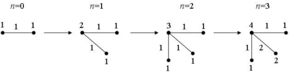
Figure 2 shows an example for the graph evolution. At the initial stepn= 0 we have an edge and two vertices. At step n= 1we add a new vertex with initial weight 1, choose an old vertex and connect them using a new edge. The initial
Figure 2: An example for the graph evolution
weight of the new edge is1and we increase the weight of the old vertex by1. Step 2 is similar to step 1. However, at stepn= 3, we do not add a new vertex, but2 old vertices interact. We choose two out of the existing vertices, then increase the weights of the vertices and the weight of the edge connecting them by 1. So we can see that the weight of a given vertex is the number of the interactions of the vertex.
Our results are confined to the 2-interactions model. To describe the main results we need the following notation. Throughout the paper0< p <1,0≤r≤1, 0≤q≤1are fixed numbers. LetX(n, d, w)denote the number of vertices of weight wand degreedafter thenth step. LetVn denote the number of vertices after the nth step.
Each vertex has initial weight1 and initial degree1. When a vertex takes part in an interaction, then its weight is increased by1 and its degree may increase by 0 or1. SoX(n, d, w)can be positive only for1≤w≤n+ 1 and1≤d≤w.
Let α1= (1−p)q, α2=pr/2, α=α1+α2,
β= (1−r) + 2 (1−p) (1−q)/p. (2.1) The following theorem describes the limiting behaviour of the relative frequency of vertices with a fixed weight and a fixed degree.
Theorem 2.1. Let 0 < p <1, q >0. Assume that at least one of the following three conditions are satisfied: r >0 orr <1 or q <1. Then for any fixed w and dwith 1≤w and1≤d≤wwe have
X(n, d, w)/Vn →xd,w (2.2)
almost surely as n→ ∞, where xd,w are fixed positive numbers. Furthermore, the numbers xd,w satisfy the following recurrence relation
x1,1= 1/(α+β+ 1)>0, xd,1= 0, ford6= 1, xd,w= 1
αw+β+ 1[α1(w−1)xd,w−1+ (α2(w−1) +β)xd−1,w−1], (2.3) forw≥2,1≤d≤w. If1≤d≤w is not satisfied, thenxd,w = 0.
The following lemma states that the numbersxd,w,d= 1, . . . , w,w= 1,2, . . ., form a (proper) two-dimensional discrete probability distribution. Moreover, its marginal distributions will be the limiting distributions of the weights and the degrees, respectively.
Lemma 2.2. Letp >0and definexw=x1,w+x2,w+· · ·+xw,w forw= 1,2, . . .. Then xw, w = 1,2, . . ., are positive numbers satisfying the following recurrence relation
x1= 1
α+β+ 1, xw= α(w−1) +β
αw+β+ 1 xw−1, if w >1. (2.4) xw, w = 1,2, . . ., is a discrete probability distribution. Moreover, xd,w, d = 1, . . . , w,w= 1,2, . . ., is a two-dimensional discrete probability distribution.
Next theorem shows the scale-free property of the weights of the vertices.
Theorem 2.3. LetX(n, w)denote the number of vertices of weightwafternsteps.
Assume that the conditions of Theorem 2.1 are satisfied. Then for allw= 1,2, . . . we have
X(n, w)/Vn→xw (2.5)
almost surely, as n→ ∞, where xw,w= 1,2, . . ., are positive numbers satisfying the recurrence relation (2.4). Moreover,
xw∼Cw−(1+α1) as w→ ∞ (2.6) with C=Γ
1 + β+1α αΓ
1 +αβ .
Our main result is the scale-free property of the degrees.
Theorem 2.4. Assume that the conditions0< p <1,q >0, andr >0are satis- fied. Let us denote byU(n, d)the number of vertices of degreedafternsteps, that is U(n, d) =P
w:d≤w≤n+1X(n, d, w). Then, for any d≥1we have U(n, d)
Vn →ud (2.7)
a.s. asn→ ∞, whereud=P
wxd,w,d= 1,2, . . ., are positive numbers. Further- more,
ud∼ Γ
1 + β+1α α2Γ
1 +βα α
α2
−(1+α1)
d−(1+1α) as d→ ∞. (2.8)
3. Proofs and auxiliary results
The following lemma contains the basic equation of the paper. LetFn−1denote the σ-algebra of observable events after (n−1) steps. We compute the conditional expectation ofX(n, d, w)with respect toFn−1 forw≥1.
Lemma 3.1.
E(X(n, d, w)|Fn−1) =X(n−1, d, w)
1−αw
n −β p Vn−1
+ (3.1)
+X(n−1, d, w−1)(1−p)
"
qw−1
n + (1−q) d
Vn−1
2
# +
+X(n−1, d−1, w−1)
"
p
rw−1
2n + (1−r) 1 Vn−1
+ (1−p)(1−q)Vn−1−d
Vn−1 2
# + +pδd,1δw,1.
Here δa,b denotes the Dirac-delta.
Proof. The probability that an old vertex of weightwtakes part in the interaction at stepnis
p
rw
2n+ (1−r) 1 Vn−1
+ (1−p) qw
n + (1−q)Vn−1−1
Vn−1 2
!
=w
nα+ p Vn−1
β, where αand β are defined by (2.1). So the terms at the right hand side of (3.1) correspond to the following cases. The first term covers the case when neither the degree nor the weight of a vertex change. Its probability is 1−
αw n +βVp
n−1
. The second term covers the case when the degree does not change but the weight is increased by 1, while the third term correspond to the case when both the degree and the weight are increased by 1. A new vertex always takes part in the interaction. At each step, with probabilityp, a new vertex with weight 1 and with degree 1 is born. This explains termpδd,1δw,1 in (3.1).
We shall need the following results on discrete time martingales. Let{Zn,Fn} be a submartingale. Its Doob-Meyer decomposition is Zn = Mn +An, where {Mn,Fn}is a martingale and{An,Fn} is an increasing predictable process. Here, up to an additive constant,
An =EZ1+ Xn i=2
(E(Zi|Fi−1)−Zi−1).
We see that {Mn2,Fn} is again a submartingale. Let Mn2=Yn+Bn
be the Doob-Meyer decomposition ofMn2. Here, up to an additive constant, Bn =
Xn i=2
D2(Zi|Fi−1) = Xn i=2
E
(Zi−E(Zi|Fi−1))2|Fi−1 .
Proposition 3.1 (Propositions VII-2-3 and VII-2-4 of [12]). Let M1 = 0. On the set {B∞ < ∞} the martingale Mn almost surely converges to a finite limit.
Moreover, Mn= o(Bn1/2logBn)almost surely on the set {Bn→ ∞}. A consequence of the above proposition is the following.
Proposition 3.2(Proposition 2.3 of [1]). Let{Zn,Fn}be a square integrable non- negative submartingale. IfBn1/2logBn= O(An), thenZn∼An asn→ ∞, almost surely on the set {An → ∞}.
Proof of Theorem 2.1. Applying the Marcinkiewicz strong law of large numbers to the number of vertices, we obtain
Vn=pn+ o
n1/2+ε
(3.2) almost surely, for anyε >0. Let
c(n, w) = Yn i=1
1−αw
i − βp Vi−1
−1
. Then (3.2) and Taylor’s expansion imply that
c(n, w)∼awnαw+β (3.3)
almost surely as n→ ∞, whereaw is a positive random variable.
LetZ(n, d, w) = c(n, w)X(n, d, w). Then, by (3.1), (Z(n, d, w),Fn) is a non- negative submartingale. We shall apply the Doob-Meyer decompositions Zn = Mn+An andM2=Yn+Bn. Then
A(n, d, w) =EZ(1, d, w)+
+ Xn i=2
c(i, w)X(i−1, d, w−1)(1−p) qw−1
i + (1−q) d
Vi−1
2
! + +
Xn i=2
c(i, w)X(i−1, d−1, w−1)×
×
"
p
rw−1
2i + (1−r) 1 Vi−1
+ (1−p)(1−q)Vi−1−d
Vi−1
2
# + +
Xn i=2
c(i, w)pδd,1δw,1. (3.4)
Moreover
B(n, d, w) = Xn i=2
D2(Z(i, d, w)|Fi−1)≤
≤ Xn i=2
c(i, w)2E{(X(i, d, w)−X(i−1, d, w))2|Fi−1} ≤
≤4 Xn i=2
c(i, w)2= O
n2(αw+β)+1
. (3.5)
We use induction on w. Let w = 1. We see that a vertex of weight 1 took part in an interaction only when it was born. Therefore its degree must be equal to1.
By (3.4),
A(n,1,1)∼p Xn i=2
c(i,1)∼p Xn i=2
a1iα+β∼pa1 nα+β+1
α+β+ 1 (3.6) a.s. asn→ ∞. By (3.5), B(n,1,1) = O n2(α+β)+1
and therefore (B(n,1,1))12logB(n,1,1) = O (A(n,1,1)). It follows from Proposition 3.2 that
Z(n,1,1)∼A(n,1,1) a.s. on the event {A(n,1,1)→ ∞}asn→ ∞. (3.7) As, by (3.6), A(n,1,1)→ ∞a.s., therefore using the asymptotic behaviour of Vn
andc(n, w), relation (3.7) implies X(n,1,1)
Vn
= Z(n,1,1)
c(n,1)Vn ∼ A(n,1,1)
c(n,1)Vn ∼pa1nα+β+1 α+β+1
a1nα+βpn = 1
α+β+ 1 =x1,1>0 almost surely. So (2.2) is valid forw= 1.
Suppose that the statement is true for all weights less thanwand for all possible degrees. It implies thatX(n, d, w−1)∼xd,w−1np.
Then by (3.2), (3.3) and using the induction hypothesis, we have for anyw >1 A(n, d, w)∼
Xn i=2
c(i, w)xd,w−1pi(1−p)qw−1
i +
+c(i, w)xd−1,w−1pi
pr(w−1)
2i +p(1−r)
pi + 2 (1−p) (1−q) pi
∼
∼ Xn i=2
awiαw+β
xd,w−1p(1−p)q(w−1) + +xd−1,w−1
1
2p2r(w−1) +p(1−r) + 2 (1−p) (1−q) ∼
∼paw
nαw+β+1 αw+β+ 1
(1−p)q(w−1)xd,w−1+ +
1
2pr(w−1) + (1−r) +2 (1−p) (1−q) p
xd−1,w−1
. (3.8)
In the above computation we deleted all terms having asymptotically smaller degree than the largest one.
Formula (3.8) impliesA(n, d, w) ∼pawnαw+β+1xd,w → ∞, because xd,w >0, where, by (3.8),
xd,w = 1
αw+β+ 1[α1(w−1)xd,w−1+ (α2(w−1) +β)xd−1,w−1], with α1, α2, α and β defined by (2.1). Therefore (B(n, d, w))12logB(n, d, w) = O (A(n, d, w)). So, using Proposition 3.2, we haveZ(n, d, w)∼A(n, d, w). There- fore
X(n, d, w) Vn
=Z(n, d, w)
c(n, w)Vn ∼ A(n, d, w)
c(n, w)Vn ∼ pawnαw+β+1xd,w
awnαw+βpn =xd,w (3.9) a.s. asn→ ∞.
Proof of Lemma 2.2. Ifα= 0, then the statement is obvious. Now assumeα6= 0.
Asxd,w is defined asxd,w = 0ford /∈ {1,2, . . . , w}, thereforexw=P
dxd,w. From the recurrence relation (2.3) we obtain
xw= Xw d=1
xd,w=X
d
xd,w =
= 1
αw+β+ 1
"
α1(w−1)X
d
xd,w−1+ (α2(w−1) +β)X
d
xd−1,w−1
#
=
= α(w−1) +β αw+β+ 1 xw−1.
Using this recursive formula forxw, we obtain xw=x1
Yw j=2
α(j−1) +β
αj+β+ 1 = 1 αw+β+ 1
wY−1 j=1
β α+j
β+1 α +j =
=Γ
1 +β+1α αΓ
1 + βα Γ w+αβ Γ
w+β+1α + 1. (3.10)
By [15], we have the following formula:
Xn k=0
Γ(k+a)
Γ(k+b) = 1 a−b+ 1
Γ(n+a+ 1)
Γ(n+b) − Γ(a) Γ(b−1)
. Therefore, by some calculation, we obtainPn
w=1xw→1asn→ ∞. SoP∞ w=1xw= 1. AsP
dxd,w =xw, soP∞ w=1
Pw
d=1xd,w = 1and thereforexd,w, d= 1,2, . . . , w, w= 1,2, . . ., is a (proper) two-dimensional discrete probability distribution.
Proof of Theorem 2.3. As
X(n, w) =X(n,1, w) +X(n,2, w) +· · ·+X(n, w, w),
Theorem 2.1 and Lemma 2.2 imply (2.5). Using (3.10), the Stirling formula gives (2.6).
The following representation of the joint distribution of degrees and weights is useful to prove scale-free property for degrees. Let W be a random variable with distribution P(W =w) = xw, w = 1,2, . . .. Let ξ1 ≡ 1 and ξ2, ξ3, . . . be independent random variables being independent ofW, too. Forw≥2letξwhave the following distribution:
P(ξw= 0) = α1(w−1)
α(w−1) +β, P(ξw= 1) = α2(w−1) +β α(w−1) +β . LetSw=ξ1+ξ2+· · ·+ξw.
Lemma 3.2. P(SW =d, W=w) =xd,w for all w= 1,2, . . .,d= 1,2, . . . , w.
Proof. It is easy to see that the sequence P(SW =d, W =w) satisfies the same recursion (2.3) asxd,w.
To obtain scale-free property for degrees, we need the following local limit theo- rem. LetX1, X2, . . . be independent, integer valued random variables. Letpj,m= P(Xj=m)be the distribution, whilepj,mj = maxmpj,m be the maximal value of the distribution. LetSn =Pn
i=1Xibe the partial sum,Pn(N) =P(Sn=N)be its distribution, Mn =Pn
i=1EXi be the expectation, and Bn =Pn
i=1E(Xi−EXi)2 be the variance ofSn.
Proposition 3.3 (Theorem 5 and its consequence in Section VII, 2 of [14]). As- sume that the greatest common divisor of the values
m : 1 logn
Xn j=1
pj,mjpj,m+mj → ∞
is equal to 1. Moreover,
lim inf Bn
n >0, lim sup1 n
Xn i=1
E|Xi−EXi|3<∞. Then
sup
N
pBnPn(N)− 1
√2πexp
−(N−Mn)2 2Bn
= O 1
√n
.
If we apply Proposition 3.3 to the random variablesξk in Lemma 3.2, then we obtain the following result which will play an important role in the proof our main theorem.
Proposition 3.4. Suppose that α1>0 andα2>0. Then
xd,w=xw α
√2πα1α2w
"
exp −(d−ESw)2 2D2Sw
! + O
w−12#
as w→ ∞, (3.11)
where the error termO w−12
does not depend on d.
Proof. We follow the method ofTheorem 4.2 in [3]. Letw >1. Then we have Eξw=α2(w−1) +β
α(w−1) +β = α2
α + α1β
α(α(w−1) +β), hence
ESw=Eξ1+· · ·+Eξw=wα2
α + O (logw) (3.12) as w→ ∞. By simple computation, we obtain
D2ξw= α1α2
α2 + O 1
w
, D2Sw= α1α2
α2 w+ O (logw) (3.13) as w→ ∞.
Now, we apply Proposition 3.3 forSw. The conditions of that proposition are satisfied, therefore we have
supd∈Z
DSwP(Sw=d)− 1
√2πexp −(d−ESw)2 2D2Sw
!= O 1
√w
. (3.14)
Using (3.13) and (3.14), we obtain DSw−
√α1α2w α
P(Sw=d) = O w−12
. Therefore (3.14) implies that
supd∈Z
√α1α2w
α P(Sw=d)− 1
√2πexp −(d−ESw)2 2D2Sw
!= O 1
√w
. (3.15) By the independence of W and ξi, we see that xd,w = P(SW =d, W =w) = P(Sw=d)xw. So the result follows from (3.15).
The well-known Hoeffding’s inequality is the following.
Proposition 3.5 (Theorem 2 of [11]). LetX1, X2, . . . , Xn be independent random variables,ai≤Xi ≤bi(i= 1,2, . . . , n). LetX¯ = (X1+X2+· · ·+Xn)/n,µ=EX¯. Then for any t >0
P( ¯X−µ≥t)≤exp
−2n2t2 Pn
i=1(bi−ai)2
.
Proof of Theorem 2.4. Theorem 2.1 and Lemma 2.2 will imply (2.7). Hoeffding’s inequality, Lemma 3.2 and Proposition 3.4 will imply (2.8).
By Theorem 2.1 and Lemma 3.2, X(n, d, w)
Vn converges almost surely to the distributionxd,w =P(SW =d, W =w). But the cardinalities of terms in the sum P
w:d≤w≤n+1X(n, d, w)are not bounded whenn→ ∞. However, using thatxd,w, d= 1,2, . . . , w, w= 1,2, . . . is a proper two-dimensional discrete distribution, the convergence of the marginal distributions is a consequence of the convergence of the two-dimensional distributions. So we obtain (2.7).
To obtain (2.8), we can apply the method ofTheorem 4.3 in [3]. Let f = α
α2
d , H =Hd=n
w:f−f12+ε≤w≤f+f12+εo , H−=Hd− =n
w:w < f−f12+εo
, H+=Hd+=n
w:w > f +f12+εo with some fixed0< ε <1/6.
Using (3.12) and Proposition 3.5, we obtain forw∈H− P(Sw=d)≤P(Sw≥d)≤P
Sw−ESw≥d−α2
αw−O (logw)
≤
≤exp
−2 w
d−α2
αw−O (logw)2
= exp (
−2α2
α
2(f−w−O (logw))2 w
) . Noww∈H− implies that
(f−w−O (logw))2= (f −w)2−2 (f −w) O (logw) + (O (logw))2≥
≥f1+2ε−O (flogf). Therefore in the case whenw∈H− we obtain
P(Sw=d)≤exp
−2α2
α
2f1+2ε−O (flogf) f
=
= exp
−2α2
α 2
f2ε+ O (logf)
. This implies that
P SW =d, W∈H−
= X
w∈H−
P(Sw=d, W =w)≤ X
w∈H−
P(Sw=d)≤
≤fexp
−2α2
α 2
f2ε+ O (logf)
= o
f−(1+α1)
. (3.16)
In the case whenw∈H+, by Hoeffding’s inequality, we have P(Sw=d)≤P(Sw≤d)≤P
Sw−ESw≤d−α2
αw
≤
≤exp
−2 w
d−α2
αw2
= exp (
−2α2
α
2(f−w)2 w
) . Because w∈H+ and 12 +ε <1, we obtain 2 (w−f)≥f12+ε+w−f ≥f12+ε+ (w−f)12+ε≥w12+ε. So
P(Sw=d)≤exp
−2α2
α
2w1+2ε 4w
= exp
−1 2
α2
α 2
w2ε
. Therefore
P SW =d, W ∈H+
≤ X
{w:f <w}
exp
−1 2
α2
α 2
w2ε
= o
f−(1+α1)
. (3.17) Now turn to the case ofw∈H =Hd. Consider the set
B ={(d, w) : w≥1, d≥1, w∈Hd}. It is easy to see that
if d→ ∞ and (d, w)∈B, then w d →1.
Asw∈H, so we havew=f + O f12+ε
. Then (withε1>0 arbitrarily small)
−(d−ESw)2 2D2Sw
=−
d−wα2
α −O (logw)2
2α1α2
α2 w+ O (logw) =−α2
α1
(f−w−O (logw))2 2w+ O (logw) =
=−α2
α1
(f−w)2+ O
f12+ε+ε1
2w+ O (logw) =−α2
α1
(f−w)2 2f + O
f−12+3ε
(3.18) asd→ ∞. Here the error term does not depend onw. By (3.11), (2.6) and (3.18), we obtain
xd,w∼
∼Cw−(1+α1) α
√2πα1α2w
"
exp (
−α2
α1
(f −w)2 2f + O
f−12+3ε) + O
w−12#
∼
∼Cf−(1+α1)α α2
q 1
2παα12f exp (
−(f −w)2 2αα12f
)
as d→ ∞andw∈H, whereC=Γ
1 +β+1α /
αΓ
1 + βα
. Therefore X
w∈H
xd,w ∼ X
f−f12+ε<w<f+f12+ε
Cf−(1+α1) α α2
q 1 2παα1
2f exp (
−(f−w)2 2αα12f
)
=
=Cf−(1+α1) α α2
X
−f12+ε<k<f12+ε
q 1
2παα12f exp (
− k2 2αα12f
)
=
=A X
−fε<√kf<fε
√1f q 1
2παα1
2
exp
− √k
f
2
2αα12
→
→A
+∞
Z
−∞
q 1 2παα12
exp (
− x2 2αα12
)
dx=A,
where
A= Γ
1 + β+1α α2Γ
1 +αβ αd
α2
−(1+α1) . So we obtain
P(SW =d, W∈H)∼ Γ
1 + β+1α α2Γ
1 +αβ αd
α2
−(1+α1)
(3.19)
as d→ ∞. Finally, by (3.16), (3.17) and (3.19), we obtain
ud∼ Γ
1 + β+1α α2Γ
1 +αβ α
α2
d
−(1+α1)
as d→ ∞.
References
[1] Backhausz, Á.,Analysis of random graphs with methods of martingale theory.PhD thesis, Eötvös Loránd University, Budapest, 2012.
[2] Backhausz, Á., Móri, T. F., A random graph model based on 3-interactions.
Ann. Univ. Sci. Budapest. Sect. Comput.Vol. 36 (2012), 41–52.
[3] Backhausz, Á., Móri, T. F.,Weights and degrees in a random graph model based on 3-interactions.Acta Math. Hungar.Vol. 143 (2014), no. 1, 23–43.
[4] Barabási, A.L., Albert, R., Emergence of scaling in random networks.Science, Vol. 286 (1999), 509–512.
[5] Bollobás, B., Riordan, O., Spencer, J., Tusnády, G., The degree sequence of a scale-free random graph process.Random Structures Algorithms, Vol. 18 (2001), 279–290.
[6] Cooper, C., Frieze, A.,A general model of web graphs. Random Structures Al- gorithms, Vol. 22 (2003), 311–335.
[7] Durrett, R., Random graph dynamics. Cambridge University Press, Cambridge UK, 2007.
[8] Fazekas, I., Porvázsnyik, B., Scale-free property for degrees and weights in a preferential attachment random graph model.Journal of Probability and Statistics, Vol. 2013 (2013), Article ID 707960.
[9] Fazekas, I., Porvázsnyik, B., Scale-free property for degrees and weights in an N-interaction random graph model.arXiv:1309.4258v1 [math.PR] 17 Sep. 2013.
[10] Grechnikov, E., An estimate for the number of edges between vertices of given degrees in random graphs in the Bollobás-Riordan model. Mosc. J. Comb. Number Theory, Vol. 1 (2011), no. 2, 40–73.
[11] Hoeffding, W.,Probability inequalities for sums of bounded random variables.J.
Amer. Statist. Assoc., Vol. 58 (1963), 13–30.
[12] Neveu, J.,Discrete-parameter martingales.North-Holland, Amsterdam, 1975.
[13] Ostroumova, L., Ryabchenko, A., Samosvat, E., Generalized preferen- tial attachment: tunable power-law degree distribution and clustering coefficient.
arXiv:1205.3015v1 [math.CO] 14 May 2012.
[14] Petrov, V. V.,Sums of Independent Random Variables.Akademie-Verlag, Berlin, 1975.
[15] Prudnikov, A. P., Brychkov, Yu. A., Marichev, O. I., Integrals and series.
Gordon & Breach Science Publishers, New York, 1986.
[16] van der Hofstad, R.,Random Graphs and Complex Networks.Eindhoven Univer- sity of Technology, The Netherlands, rhofstad@win.tue.nl, 2013.
[17] Yule, G. U.,A Mathematical Theory of Evolution, Based on the Conclusions of Dr.
J. C. Willis, F.R.S.Phil. Transact. Royal Society London, Ser. B, Vol. 213 (1925), 21–87.