Methods to analysis of queueing models with state-dependent jump priorities
Agassi Melikov
a, Anar Rustamov
bTuran Jafarzade
c, János Sztrik
daInstitute of Control Science agassi.melikov@rambler.ru
bQafqaz University anar.rustemov@gmail.com
cNational Aviation Academy turan_jafarzade@hotmail.com
dUniversity of Debrecen sztrik.janos@inf.unideb.hu
Submitted April 20, 2016 — Accepted September 7, 2016
Abstract
In this paper, exact and approximate approaches for studying queuing models with state-dependent jump priorities are developed. Both models with finite separate buffers and finite common buffer for heterogeneous calls are investigated. It is shown that both models might be described by two- dimensional Markov Chains (2-D MC). Exact approach based on solution of appropriate system of balance equations (SBE) for state probabilities faced with big computational challenges for large scale models. To overcome the in- dicated difficulties an approximate approach based on the state space merging algorithms is developed. This approach allows to construct simple algorithms to calculate the Quality of Service (QoS) metrics of the examined models. The results of numerical experiments are demonstrated.
Keywords: queuing models, jump priority, Markov chains, space merging, numerical analysis
MSC:60K25, 68M20, 90B22 http://ami.ektf.hu
143
1. Introduction
Priorities are effective tools to solve the problems of quality of service (QoS) provi- sioning of heteregeneous calls in queuing systems. By nature the priorities can be broadly divided into two classes: static anddynamic. Static priorities (relative or preemptive) are defined in advance and they do not change during the whole system operation time [1]. In literature relative static priorities in queuing systems with buffers sometimes are called HOL-priorities (Head-Of-Line), .i.e. in static priorities call for service is chosen from the head of line according to the highest priority.
Dynamic priorities in turn are divided into two classes: dynamical vs time and dynamical vs state. In dynamical versus time priorities the priority of the calls can be changed according their waiting times (or sojourn time) [2]. Indynamical versus state priorities (they sometimes are called state-dependent priorities) calls can change priority according the state of the system where the state is described by vector whose components indicate number of heterogeneous calls in the queue (or in the system) [3].
The drawback of static priorities is that when they are used in real systems the delay of low priority calls is too large espesially for the system with heavy loads of high priority calls. Dynamic priorities allow to avoid the starvation of low priority calls. Detailed review of priority schemas might be found in [4].
As a rule, classical priorities (static or dynamic) are used to determine type of call from the buffer which must be send to channel for servicing. However, some scientific and practical interest represents the priorities which are introduced to change (either increase or decrease) the priorities of calls in buffer. These changes are realized instantaneously so such kind of priorities are called jump priorities (JP). They might be either static or dynamic too. Let us breifly review existing results related to such kind of priorities.
The pioneer work on the analyzing dynamical vs time HOL-priorities with prior- ity jumps (HOL-JP) is [5]. In this paper dynamical vs time HOL-JP was proposed where calls with low priority can jump to another buffer with high priority after waiting some (deterministic) period of time in native buffer; this process goes until a call of any type gets access to a channel or reaches a queue with highest priority.
Formulas for calculation of the mean waiting time of the heterogeneous calls were developed in [5].
Dynamical vs state HOL-JP in discrete-time queuing models were proposed in [6-10]. In these models authors included two kinds of calls - high priority calls (H- calls) and low priority calls (L-calls). A scheme of head-of-line merge-by-probability (HOL-MBP) according to which at the end of each time slot all L-calls go to the end of the queue of H-calls with the fixed probabilityβ,0< β <1, was proposed in [6]. A modification of the HOL-MBP scheme was considered in [7]. It was named head-of-line jump-or-serve (HOL-JOS) and, in contrast to the scheme of [6]], in it only one L-call goes from the queue head into the H-queue. Unlike the HOL- JOS scheme, in HOL-JIA1 (Head-Of-Line Jump If-Arrival) scheme [8] transition of the L-call into the H-queue depends not only on the state of the H-queue at
the beginning of the slot, but also on the number of arrivals of L-calls during this slot. The only distinction of the HOL-JIA1 scheme from the HOL-JIA2 scheme [9] lies in that in the latter scheme the L-calls can pass immediately to the H- queue. Formulas for the generating functions of the call queue lengths of both types and the time of H-call waiting on the queue, as well as their moments, were developed in [6-10]. Additionally, the mean time of waiting in the queue of L-calls was determined.
In [5-10] queuing models with infinite buffers are investigated. So, they have little applicability in the real communication networks. In particular, real commu- nication networks have finite buffer capacity. Secondly, investigated JP are defined by state-independent probabilities. Since they cannot be adapted for real situations depending on loads of heterogeneous calls.
Different approach to study queuing models with dynamical vs state HOL- JP can be found in the papers [11–14] and in chapter 5 of the book [15] where new type of randomized state-dependent JP for continuous-time queuing systems with finite buffers was proposed. In papers [11, 12] models with separate buffers for heterogeneous calls have been examined while in paper [13, 14] models with common buffer are investigated. They make it possible pass to from the L-queue into the H-queue only at the instants of arrival of the L-calls, the probability of such transitions depend only on the number of L-calls in the system. In chapter 5 of the book [15] models with separate buffers which jump priorities depending only on the number of H-calls in the system were examined. In the indicated works [11–14] methods of calculation of main QoS metrics of the investigated models are proposed. To the best of our knowledge, models in which JP depends on the number of both types of calls in the system are not examined. In this paper we investigate such kinds of models.
At the end of this section it’s worth noting that in [16] queueing models with finite common buffer and two priority classes of calls are investigated, where it is assumed that H-calls can preempt the service of L-calls. Futhermore in [16]
various congestion control mechanisms are also proposed. In order to calculate the steady-state probabilities of the investigated models, new calculation approach of the original method based on the theory of generalized invariant subspace is developed. Unlike [16] preemption of H-calls from the services of L-calls is not allowed in our paper. However L-call can jump H-buffer in order to served as H-calls.
The rest of the paper is organized as follows. In section 2 model with separate buffers and state-dependent JP is examined and both exact and approximate meth- ods of calculation its QoS metrics are developed. Similar problems for model with common buffer are investigated in section 3. Section 4 is about numerical results of models with both separate buffers and common buffer. In numerical experiments, we investigate different schemas of changing elements of JP-matrix. Conclusion remarks are given in section 5.
2. Jump priorities in model with separate buffers
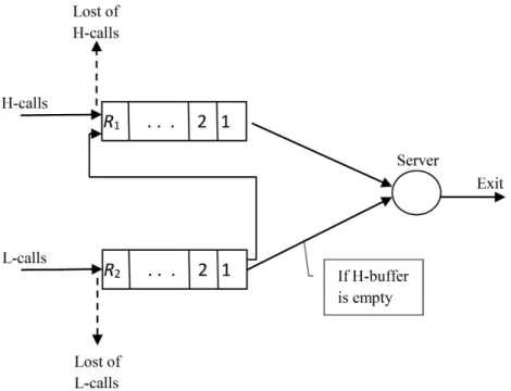
The structure scheme of the studied queuing system is depicted in Figure 1. In the single server queueing system two Poisson traffic of heterogeneous calls have different arrival rateλi, i= 1,2. We determined first type of calls as high priority calls (H-calls) while second type of calls are treated as low priority calls (L-calls).
By default H-call from the buffer dominating to be served by the idle server; only in the case of absence of H-call in the buffer, L-calls can be served. If there isn’t any call in the buffer, then the channels becomes free. Service intensity of the server is the same for both type of the call where it is determined asµobeying exponential distribution.
Figure 1: Structure of the queuing system with jump priorities
First let us consider the model with separate buffers, i.e. it is assumed that there are two isolated buffers – H-buffer (for waiting H-calls) and L-buffer (for waiting L-calls) with size ofR1 andR2(0< Ri<∞, i= 1,2)respectively.
Decision epochs (i.e. jumping moments of L-calls to H-buffer) coincide with the arrival moments of L-calls. In this model state-dependent HOL-JP is defined as follows:
• High priority calls are always accepted to the H-buffer with the probability 1 if there is a free place in this buffer. If the H-buffer is full then arrived H-call will be dropped with probability 1.
• If upon arrival L-call number of calls of this type equalsi, i < R2, and number of H-call equalsj, j < R1, then L-call joins the H-buffer with probabilityαi(j) and in future it will be served as H-call; and arrived L-call joins the L-buffer with probability1−αi(j).
• If upon arrival L-call number of H-call equals R1, then L-call joins the L- buffer if there is free place in this buffer; otherwise, arrived L-call will be dropped with probability 1.
• If upon arrival L-call L-buffer is full and number of H-call equalsj, j < R1, then L-call joins the H-buffer with probabilityαR2(j); and arrived L-call will be dropped with probability1−αR2(j).
In other words, to define JP matrix with dimension (R2+ 1)xR1 is introduced.
Entities of this matrix (JP-matrix) areαi(j), i= 0,1, . . . , R2, j= 0,1, . . . , R1−1.
Thus in this scheme entities of JP-matrix depends on both number of heterogeneous calls in the appropriate buffers.
Let us note some important special schemes regarding the jump priorities men- tioned above.
1)The uniform schemas. In this schemas, the elements of JP-matrix does not depend on the number of heteregeneous calls in the buffers. So, if the elements of JP-matrix does not depend on the number of H-calls in the buffer, i.e.,αi(j) =αi
for any j = 0,1, . . . , R1−1, then we obtain JP-schema which was proposed in [11, 12]. Here in the special case αi = 0, we obtain the classical HOL-priorities.
Alternative case is that the elements of JP-matrix do not depend on the number of L-calls in the buffer, i.e.,αi(j) =α(j)for anyi= 0,1, . . . , R2. Such kind of JP has been investigated in [15]. In last scheme in the special case α(j) = 1 for any i= 0,1, . . . , R2, we obtain the classical queuing system with single traffic.
2) The threshold-based schemas. In these schemas, the threshold parameters Ti,0≤Ti≤R1−1, i= 0,1, . . . , R2, are introduced, and elements of JP-matrix are defined as follows:
αi(j) =
αi1, if 0≤j≤Ti, αi2, if j > Ti.
The probabilitiesαij, i= 0,1, . . . , R2, j = 1,2,can be defined in various ways.
In special cases, i.e. when these probabilities equal either 0 or 1 we obtain different non-randomized threshold-based JP-schemas.
The problem is finding the QoS metrics for this model. The main QoS metrics are the following: the stationary probability of lossing the calls of the ith type (CLPi), the mean number of the ith type calls in the buffers (Li) and the mean call transmission delay of theith type calls (CTDi),i=1, 2.
2.1. Exact method for model with separate buffers
The state of the system is defined by two dimensional vectors n= (n1, n2)where the first component indicates the number of H-calls and the second one the number
of L-calls respectively. In other words, operation of this system is described by the two-dimensional Markov Chain (2-D MC) with the following state space:
S={n: ni = 0,1, . . . , Ri, i= 1,2}. (2.1) Transition intensity from staten∈S to staten0∈S are denoted byq(n, n0).
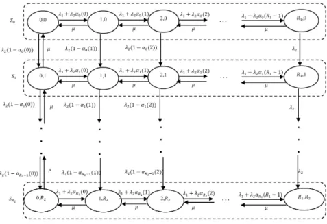
Then nonnegative elements of the generating matrix (Q-matrix) of the given 2-D MC can be calculated as below (see Figure 2):
Figure 2: State diagram of the model with separate buffers
q(n,n0) =
λ1+λ2αn2(n1), if n1< R1, n0 =n+e1,
λ2(1−αn2(n1)), if n1< R1, n2< R2, n0=n+e2, λ2, if n1=R1, n0=n+e2,
µ, if n1>0, n0=n−e1 or n1= 0, n0=n−e2,
0 in other cases,
(2.2)
wheree1= (1,0), e2= (0,1).
For any positive values of the parameters of incoming traffics, all states of the investigated finite MC are communicating (see Figure 2), and consequently, stationary distribution of the investigated 2-D MC exists.
The stationary probability of state n ∈ S is denoted by p(n). Construction and solution of the corresponding system of balance equations (SBE) for the given
2-D MC is the standard way for determining the stationary state probabilities. It is constructed with regard to (2.2) and has the following form:
Casen1< R1, n2< R2:
p(n1, n2) (λ1+λ2+µI(n1+n2>0)) = p(n1−1, n2)I(n1>0) (λ1+λ2αn2(n1−1)) + p(n1, n2−1)I(n2>0)λ2(1−αn2−1(n1)) + p(n1+ 1, n2)µ+p(n1, n2+ 1)µI(n1= 0)
(2.3)
Casen1=R1, n2< R2: p(R1, n2) (µ+λ2) =
p(R1−1, n2) (λ1+λ2αn2(R1−1)) +p(R1, n2−1)I(n2>0)λ2; (2.4) Casen2=R2:
p(n1, R2) (µ+λ1+λ2αR2(n1)I(n1< R1)) =
p(n1−1, R2)µI(n1>0) +p(n1, R2−1)2(1−αR2−1(n1)) . (2.5) The SBE (2.3)–(2.5) should be completed with normalizing condition over state space (2.1):
X
n∈S
p(n) = 1. (2.6)
After determining the state probabilities from SBE (2.3)–(2.6), one can establish its QoS metrics. As indicated above, H-calls are lost if upon their arrivals H-buffer is full. Hence, the loss probability for H-calls (CLP1) can be determined as follows:
CLP1=
R2
X
i=0
p(R1, i). (2.7)
Similarly, we conclude that L-calls are lost in the following cases: (2.1) at the time an L-call arrives, both buffers are full (in such case L-call is lost with probability 1); (2.2) at the time an L-call arrives, L-buffer is full but there is free place in H-buffer (in such case L-call is lost with probability1−αR2(i)). Thus the loss probability of L-calls (CLP2) is given by
CLP2=p(R1, R2) +
RX1−1 i=0
p(i, R2) (1−αR2(i)). (2.8) The first and second terms of the sum in the formula (2.8) denote the probability of events (2.1) and (2.2), respectively.
The mean numbers of the H-calls (L1) and L-calls (L2) in the queue are deter- mined as the expected values of appropriate discrete random variables:
L1=
R1
X
i=1
i
R2
X
j=0
p(i, j); (2.9)
L2=
R2
X
i=1
i
R1
X
j=0
p(j, i). (2.10)
Further, formulas (2.3)–(2.6) and modified Little’s formula can be used to eval- uate the mean times of transmission delay for the heterogeneous:
CT D1= L1
λ(c)1 ; (2.11)
CT D2= L2
λ(c)1 +λ(c)2 , (2.12)
where λ(c)1 and λ(c)2 are carried loads of H-calls and L-calls, respectively. These parameters are calculated as follows:
λ(c)1 =λ1
1−
R2
X
j=0
p(R1, j)
+λ2 RX1−1
i=0 R2
X
j=0
p(i, j)αj(i);
λ(c)2 =λ2 R1
X
i=0 RX2−1
j=0
p(i, j) (1−αj(i)).
Thus, to find QoS metrics (2.7)–(2.12), it is necessary to determine the steady- state probabilities of the model from the corresponding SBE (2.3)–(2.6). By im- plementation of programming languages it is possible to solve the SBE (2.3)–(2.6) for the steady-state probabilitiesp(n),n∈Swith a help of numerical methods of the linear algebra. This method of calculation of QoS metrics is called the exact (precise) method. In cases of moderate capacity of state space (2.1) this methods is reasonable to calculate QoS metrics of the system. But for large scale system (i.e. when system has large buffers) it isn’t suitable. Therefore, we need to find out a more efficient method to calculate the QoS metrics of the models with large buffers.
2.2. Approximate method for model with separate buffers
Below we consider asymptotic analysis of the QoS metrics for large scale models, i.e. when R1 and R2 take large values. The developed approximate method has high accuracy for heavy traffic regime of H-calls. In other words, below we consider asymptotic analysis of the large scale model with heavy loads of H-calls, i.e. it is assumed thatν1 ν2,whereνi =λi/µ, i= 1,2. Note that this assumption is not something extraordinary because introduction of the jump priorities for the L-calls makes sense, namely in the systems with heavy loads of H-calls.
Consider the following splitting of the state space (2.1):
S=
R2
[
i=0
Si, Si
\Sj =∅, i6=j, (2.13)
whereSi={n∈S:n2=i}, i= 0,1,2, . . . , R2.
We notice that the assumption made about the relation of the loads of the het- erogeneous calls enables one to satisfy the condition for correct use of the algorithms of state space merging of the 2-D MC (see [3, Appendix]): transition intensities within classesSi, i= 0,1, . . . , R2,are essentially higher than those between states of different classes.
The classes of microstates Si are united into individual merged states < i >, and in the original state spaceS the following merge function is defined:
U(n) =< i >, if n∈Si . (2.14) The function (2.14) defines a merged model with the state space
Ω ={< i >:i= 0,1,2, . . . , R2}.
Let us consider the problem of calculation of state probabilities inside the split- ting models. The stationary probability of the state(k, i)in the split model with the state space Si is denoted by ρi(k), i= 0,1,2, . . . , R2, k = 0,1,2, . . . , R1.
Each split model with state space Si is a one-dimensional birth and death process with the parameters that are calculated as follows (see Figure 2):
qi(k1, k2) =
λ1+λ2αi(k1), if k2=k1+ 1
µ, if k2=k1−1
0, otherwise.
(2.15) Consequently, we have
ρi(k) =
kY−1 j=0
(ν1+ν2αi(j))ρi(0), k= 1, . . . , R1, (2.16)
whereρi(0) =
1 +PR1
k=1
Qk−1
j=0(ν1+ν2αi(j))−1
.
The elements of the Q-matrix of the merged model are denoted by q(< k >, < k0 >), < k >, < k0>∈Ω.
According to the algorithm of state space merging of the 2-D MC (see [3, Ap- pendix]) these elements are given by
q(< k >, < k0>) = X
n∈Sk
n0∈Sk0
q(n,n0)ρn1(n2). (2.17)
So, by using (2.2), (2.16) and (2.17) after some mathematical transformations the following formula are obtained (see Figure 2):
q(< k >, < k0>) =
λ2
ρk(R1) +PR1−1
i=0 (1−αk(i))ρk(i)
, if k0=k+ 1,
µρk(0), if k0=k−1,
0 otherwise.
(2.18)
From (2.18) we can calculate the probabilities of the merged states π(< k >), < k >∈Ω
as follows:
π(< k >) =ν2k kY−1 j=0
Λjπ(<0>), k= 1, . . . , R2, (2.19) where
π(<0>) =
1 +
R2
X
k=1
ν2k k−1Y
j=0
Λj
−1
,
Λj =ρj(R1) +PR1−1
i=0 (1−αj(i))ρj(i)
ρj+1(0) , j= 0, . . . , R2−1.
The state probabilities of the initial 2-D MC are determined approximately as follows (see [3, Appendix]):
p(i, j)≈ρj(i)π(< j >). (2.20) By taking into account (2.16), (2.19) and (2.20) we can calculate approximate values of state probabilities of initial 2-D MC, and omitting the intermediate math- ematical calculations the following approximate formulae to calculate the QoS met- rics (2.7)-(2.10) are obtained:
CLP1≈
R2
X
i=0
ρi(R1)π(< i >) ; (2.21)
CLP2≈π(< R2>) ρR2(R1) +
RX1−1 i=0
ρR2(i) (1−αR2(i))
!
; (2.22)
L1≈
R1
X
i=1
i
R2
X
k=0
ρk(i)π(< k >); (2.23)
L2≈
R2
X
k=1
k π(< k >). (2.24) The QoS metricsCT Dk are determined from (2.11) and (2.12) after the calcu- lation of the parametersLk andλ(c)k , k= 1,2.
3. Jump priorities in models with common buffer
Now let us consider the model with common buffer. In this case it is assumed that there is single buffer with sizeR, 0< R <∞,for both types of calls. In this model the state-dependent HOL-JP is defined as follows.
• High priority calls are always accepted to the common buffer with the proba- bility 1 if there is a free place in the buffer. If the common buffer is full then arriving H-call will be dropped with probability 1.
• If upon arrival of L-call the number of H-calls equals n1 and number of L-calls equalsn2, where n1+n2 < R, then arriving L-call becomes H-call with probability βn2(n1) or it will be accepted to the buffer as L-call with probability1−βn2(n1).
• If upon arrival of L-call common buffer is full (i.e. in case n1+n2 =R) it will be dropped with probability 1.
The main QoS metrics of the model are the same with the model with separate buffers.
3.1. Exact method for model with common buffer
As it is mentioned in section 2, the 2-D vector n = (n1, n2) is used to describe the state of the system and state space for this model is determined as follows (see Figure 3):
S={n: ni = 0,1, . . . , R, i= 1,2; n1+n2=R} . (3.1) Note 1. Hereinafter, for simplicity, we use the same notations for the state spaces, state probabilities etc. in different models. This will not lead to misunder- standing since from the context it will be clear which model is being considered.
In this case the nonnegative elements of the Q-matrix of the given 2-D MC can be calculated as follows (see Figure 3):
q(n,n0) =
λ1+λ2αn2(n1), if n1+n2< R, n0=n+e1, λ2(1−αn2(n1)), if n1+n2< R, n0=n+e2,
µ, if n1>0, n0=n−e1 or
n1= 0, n0=n−e2,
0 in other cases.
(3.2)
Figure 3: State diagram of the model with common buffer
Loss probabilities of heterogeneous calls in this model equal each other and are given by
CLP1=CLP2= X
n∈Sd
p(n), (3.3)
whereSd={n∈S: n1+n2=R}is set of diagonal states (see Figure 3).
In this model the mean number of the H-calls and L-calls in the buffer are determined as follows:
Lk= XR i=1
iξk(i) (3.4)
whereξk =P
n∈Sp(n)δ(nk =i), k= 1,2; δ(i, j)are Kronecker’s symbols.
The mean transmission delays of the heterogeneous calls are determined by Eqs.
(2.11) and (2.12).
Computational difficulties of the exact approach to solve appropriate SBE (it is constructed with regard to (3.2) and here it is omitted) are observed in the models with large scale too. In order to overcome the above-mentioned computational difficulties to calculate the QoS metrics (3.3), (3.4) an approximate approach to asymptotic analysis can be applied as well.
3.2. Approximate method for model with common buffer
Similar to (2.13) splitting of the state space (3.1) is considered:
S= [R i=0
Si, Si
\Sj =∅, i6=j, (3.5)
whereSi={n∈S:n2=i}, i= 0,1, . . . , R.
Not repeating the stages of the approximate approach, final formula to calculate QoS metrics are given below. In this case stationary distribution of the split model with state spaceSi, i= 0,1, . . . , R−1, is defined as follows:
ρi(k) =
kY−1 j=0
(ν1+ν2βi(j))ρi(0), k= 1, . . . , R−i, (3.6)
whereρi(0) =
1 +PR−i k=1
Qk−1
j=0(ν1+ν2βi(j))−1
.
Note2. Split model with state spaceSRcontains only one micro-state(0, R)∈S so we setρR(0) = 1.
According to the algorithm of state space merging of the 2-D MC, the elements of the Q-matrix of the merged model in this case (see formulae (2.17), (3.2) and (3.6)) are given by
q(< k >, < k0>) =
λ2PR−k−1
i=0 ρk(i) (1−βk(i)), if k0=k+ 1,
µρk(0), if k0=k−1,
0 otherwise.
(3.7)
So, the probabilities of the merged states in this model are calculated as follows:
π(< k >) =ν2k kY−1 j=0
Mjπ(<0>), k= 1, . . . , R, (3.8)
where π(<0>) = 1 +PR
k=1ν2k Qk−1 j=0Mj
−1
, Mj =
PR−j−1
i=0 ρj(i)(1−βj(i)) ρj+1(0) , j = 0, . . . , R−1.
So, by using (3.6) and (3.8) from (2.20) we can calculate approximate values of steady-state probabilities of initial 2-D MC for the model with common buffer.
Consequently, for asymptotic analysis of QoS metrics of the investigated model the following approximate formula are obtained:
CLP1≈CLP2≈ XR
i=0
ρi(R−i)π(< i >) ; (3.9)
L1≈ XR k=1
k
R−kX
i=0
ρi(k)π(< i >) ; (3.10)
L2≈ XR k=1
k π(< k >). (3.11) Based on (3.10) and (3.11) approximate values of transmission delays of the heterogeneous calls are calculated by (2.11) and (2.12).
4. Numerical results
The developed approximate formula allow one to carry out an authentic analysis of QoS metrics over any range of change of values of loading parameters of the heterogeneous traffic, satisfying assumption concerning their ration (i.e. whenν1 ν2) and also at any buffers sizes.
Let us first examine the results of the numerical experiments for the model with separate buffers. The following initial data for hypothetical model was se- lected: R1+R2 = 110, λ1= 2, λ2= 0.5, µ= 3, i.e. ν1 = 2/3, ν2 = 1/6. The numerical results are analyzed based on the two schemas for changing the elements of JP-matrix. In schema 1 it is assumed that they are changed with respect to both parameters (state-dependent JP) and defined as αi(j) = i+j+2i+1 while in sec- ond one we assume that they are constant (state-independent JP), i.e. αi(j) = 0.5 for any i and j. In other words, in schema 1 probabilities of jumping to H- buffer are decreasing function with respect to number of H-calls in buffer at fixed values of L-calls but in schema 2 they do not depend on number of heterogeneous calls in buffers.
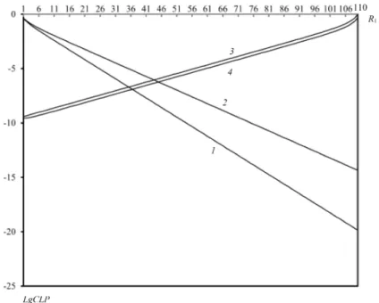
Figures 4–6 show dependences of QoS metrics onR1.As it was expected the loss probability of H-calls is positively related to the buffer size of H-buffer (Figures 4) while loss probability of L-calls is increasing function versusR1. As we see from Figures 4, rate of change of the indicated functions are high enough. Also from this figure we conclude that schema 1 is favorable for the loss probabilities of H-calls while for loss probabilities of L-calls schema 2 is favorable. Moreover, differences between values of loss probabilities of H-calls are essential in different schemas especially at large buffer sizes but values of loss probabilities of L-calls are very close to each other in different schemas.
Let us note that from this graph for both schemas we may find such values of buffer sizes for which difference between loss probabilities of heterogeneous calls is less than given>0 (such kind of problems are called-fair servicing policy).
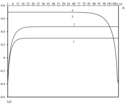
Dependency of length of heterogeneous calls on the H-buffer size is shown in Figures 5. In both schemas the mean queue length of the H-calls positively related to the H-buffer size but length of the L-calls is negatively related to the H-buffer size. From this figure we conclude that schema 1 again is favorable for length of the H-calls while length of the L-calls is invariant to different schemas. Behav- ior of the indicated QoS metrics is interesting. So, length of the H-calls in both schemas increases with low rates for small values ofR1,and for aboutR1>20they are almost constant; alternative situation occurs for length of the L-calls in both
Figure 4: Dependence of loss probabilities versusR1in model with separate buffers: 1- CLP1 inschema 1; 2-CLP1 inschema 2; 3-
CLP2inschema 1; 4-CLP2 inschema 2
schemas, i.e. they are almost constant forR1<100, and after that they decrease with low rates.
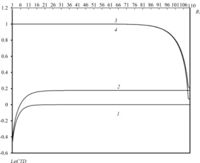
Behavior of both functions CT D1 and CT D2 are very similar to behavior of functionsL1 and L2 respectively (see Figures 6). In other words, schema 1 again is favorable for CT D1 while CT D2 is almost constant in different schemas; in both schemesCT D1 increases with low rates for small values ofR1,and for about R1>20 they are almost constant andCT D2 in both schemas is almost constant forR1<100, and forR1>100 it decreases with low rates.
Let us now consider the results for model with common buffer based on above indicated different schemas of changing of parameters αi(j), i= 0,1,2, . . . , R− 1, j= 0,1, . . . , R−i−1. Loads of this model are unchanged, i.e. we selectν1 = 2/3, ν2= 1/6.
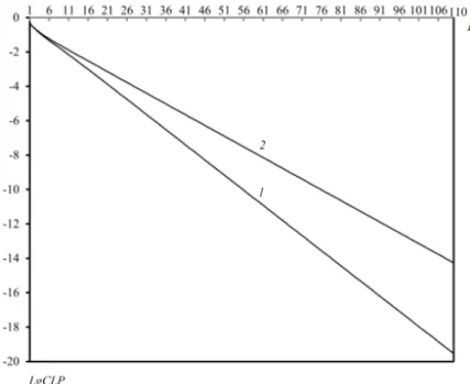
Dependency of functionCLP (as it was mentioned above loss probabilities of heterogeneous calls in this model equal each other, see (3.2)) on the buffer size is shown in Figures 7. It is seen from this figure that in both schemas the loss probability of calls strictly decreases (with high rate) versus the common buffer size and as it was expected schema 1 is favorable for the loss probabilities. Note that differences between values of loss probabilities in different schemas are increased versus buffer size.
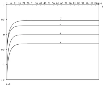
In Figures 8 the dependency of functionsL1andL2on the buffer size is shown.
Figure 5: Dependence of mean length of queues versusR1in model with separate buffers: 1-L1 inschema 1; 2-L1 inschema 2; 3-L2
inschema 1; 4-L2 inschema 2
In both schemas these functions increase versus the common buffer size. From this figure we conclude that schema 1 is favorable for length of the H-calls while schema 2 is favorable for length of the L-calls. As in case of the model with separate buffers, in this model the rate of change (increasing) of these functions are very small too, i.e. aboutR >15they are almost constant.
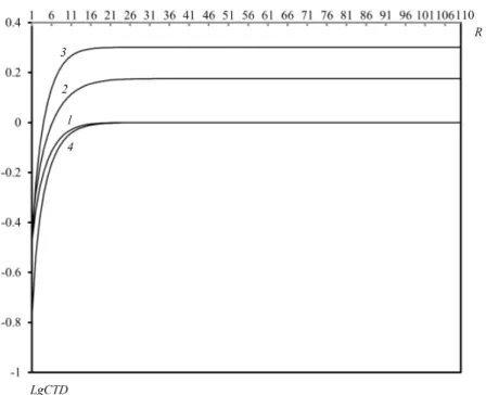
Again behavior of both functionsCT D1andCT D2 is very similar to behavior of functions L1 and L2 respectively (see Figures 9). It is interesting that in this case aboutR >15values of the functionCT D1 in schema 1 are almost same with values of the functionCT D2in schema 2.
Presented numerical results allow to take some comparisons proposed in two buffer management mechanisms. So, for instance, values of both functionsCLP1
and CLP2 in model with separate buffers equal (approximately) 10−6.5 and this value corresponds to buffers sizeR1= 35, R2= 75 (R1+R2= 110).However, the indicated value for both kinds of calls might be provided in model with common buffer at sizeR= 36.In other words, common buffer is essentially effective buffer management mechanisms for call loss probabilities. Other interesting conclusions with respect to the rest QoS metrics in different buffer management mechanisms might be carried out.
Another goal of performing numerical experiments was the estimation of the
Figure 6: Dependence mean transmission delays versusR1in model with separate buffers: 1-CT D1 inschema 1; 2-CT D1 inschema
2; 3-CT D2 inschema 1; 4-CT D2 inschema 2
proposed approximate formulae accuracy. As it was indicated in section 2, the exact values (EV) of the QoS metrics are determined by the appropriate SBE (such an approach allows studying QoS metrics of the model only for small buffer stores).
In order to be short, here in Table 1 and the results only for the model with separate buffers are demonstrated only for the schema 1 (similar results are ob- tained for the model with common buffer in both schemas as well). Here initial data was selected as above, i.e. R1+R2= 110, λ1= 2, λ2= 0.5, µ= 3.
As it is given in the tables accuracy of the proposed approximate formulae are acceptable for engineering practice. The bigger the ratiov1/v2, the higher accuracy of approximate value (AV).
5. Conclusion
This paper proposed a new class of state-dependent JP in queueing systems with finite separate buffers and finite common buffer for heterogeneous calls. An exact and effective approximate approaches for calculating the QoS metrics of heteroge- neous calls in such systems are developed. The important advantage of approximate approach lies in the use of explicit formulae to calculate the QoS metrics, which enables our approach to be used for models of any dimension. In addition, it is possible to use the proposed formulae to find the optimal (in given sense) values of
Figure 7: Dependence of loss probabilities versusR in model with common buffer: 1-schema 1, 2-schema 2
JP-matrix. Latest problems are important especially for the threshold-based non- randomized JP-schemas (see end of section 2) and they are a subject for further study.
Acknowledgements. The publication was supported by the TÁMOP-4.2.2.C- 11/1/KONV-2012-0001 project. The project has been supported by the European Union, co-financed by the European Social Fund.
Figure 8: Dependence of mean length of queues versusRin model with common buffer: 1-L1 inschema 1; 2-L1 inschema 2; 3-L2
inschema 1; 4-L2 inschema 2
R1 CLP1 L1
EV AV EV AV
15 6.76E-03 7.62E-03 1.30929 1.97560 22 1.52E-05 4.46E-05 1.64089 1.99795 29 3.63E-05 2.61E-06 1.75494 1.99984 36 8.87E-06 1.53E-07 1.79172 1.99998 43 2.21E-08 8.93E-09 1.80311 1.99999 50 5.53E-09 5.23E-10 1.80654 2 57 1.43E-10 3.06E-11 1.80756 2 64 3.58E-11 1.79E-12 1.80787 2 71 9.22E-12 1.05E-13 1.80797 2 78 2.39E-13 6.13E-15 1.80808 2 85 6.21E-14 3.59E-16 1.80844 2 92 1.63E-16 2.12E-17 1.80998 2 99 4.46E-17 1.23E-18 1.81776 2 106 1.67E-18 7.24E-20 1.87771 2
Table 1: Comparison for H-calls in model with separate buffers in schema 1
Figure 9: Dependence mean transmission delays versusRin model with common buffer: 1-CT D1inschema 1; 2-CT D1inschema 2;
3-CT D2inschema 1; 4-CT D2 inschema 2 R1 CLP2 L2
EV AV EV AV
15 3.21E-10 5.01E-09 4.193002 4.999998 22 6.25E-09 1.79E-08 4.201397 4.999992 29 4.13E-08 6.43E-08 4.196922 4.999974 36 1.93E-07 2.33E-07 4.193955 4.999914 43 7.84E-07 8.25E-07 4.192694 4.999719 50 9.02E-07 2.96E-06 4.192222 4.999098 57 1.15E-06 1.06E-05 4.192017 4.997138 64 4.36E-06 3.89E-05 4.191798 4.991074 71 1.68E-05 1.36E-04 4.191215 4.972766 78 6.61E-05 4.89E-04 4.189308 4.919352 85 2.67E-04 1.76E-03 4.182937 4.770876 92 1.13E-03 6.462E-03 4.161524 4.386067 99 5.26E-03 2.53E-02 3.08775 3.484102 106 1.20E-02 1.34E-01 1.795528 1.640507 Table 2: Comparison for L-calls in model with separate buffers in
schema 1
References
[1] Jaiswal HK. Priority queues. New York,Academic Press (1968).
[2] Kleinrock L. A delay dependent queue discipline.Naval Research Logistics Quarterly Journal, Vol. 11 (1964), 329–341.
[3] Melikov A, Ponomarenko L, Kim CS., Performance Analysis and Optimization of Multi-Traffic on Communication Networks. Heidelberg: Springer (2010).
[4] Wittevrongel S, De Vuyst S, Sys C, Bruneel H., A reservation-based scheduling mechanism for fair QoS provisioning in packet-based networks. In: Proceeding of the 26th IEEE International Teletraffic Congress, Karlskrona (2014), 55–62.
[5] Lim Y, Kobza JE., Analysis of delay dependent priority discipline in an inte- grated multiclass traffic fast packet switch,IEEE Transactions on Communication, Vol. 38(5)(1990),659–665.
[6] Maertens T, Walraevens J, Bruneel H., On priority queues with priority jumps, Performance Evaluation, Vol. 63(12)(2006): 1235–1252.
[7] Maertens T, Walraevens J, Bruneel H., A modified HOL priority schedul- ing discipline: performance analysis, European Journal of Operation Research, Vol. 180(3)(2007): 1168–1185.
[8] Maertens T, Walraevens J, Moeneclaey M, Bruneel H., A new dynamic priority scheme: performance analysis, In: Proceeding of the 13th International Conference on Analytical and Stochastic Modeling Techniques and Applications, Bonn (2006), 74–84.
[9] Maertens T, Walraevens J, Bruneel H., Performance comparison of several priority schemes with priority jumps, Annals of Operation Research, Vol.! 162 (2008), 109–
125.
[10] Walraevens J, Steyaert B, Bruneel H., Performance analysis of single-server ATM queue with priority scheduling, Computers and Operation Research, Vol. 30(12)(2003), 1807–1829.
[11] Melikov AZ, Ponomarenko LA., Kim CS., Algorithmic approach to analysis of queu- ing system with finite buffers and jump priorities,Journal of Automation and Infor- mation Sciences, Vol. 44(12)(2012),43–54.
[12] Kim CS, Oh Y, Melikov AZ., A space merging approach to the analysis of the per- formance of queueing models with buffers and priority jumps,Industrial Engineering and Management Systems, Vol. 12(3)(2013),274–280.
[13] Melikov AZ, Ponomarenko LA, Kim CS., Approximate method for analysis of queu- ing models with jump priorities,Automation and Remote Control, Vol. 74(1)(2013), 62–75.
[14] Melikov AZ, Ponomarenko LA, Kim CS., Numerical method for analysis of queuing models with priority jumps, Cybernetics and System Analysis, Vol. 49(1)(2013), 55–61.
[15] Melikov A., Ponomarenko L., Multidimensional queueing models in telecommunica- tion networks,Heidelberg: Springer, (2014).
[16] Tran HT., Do TV., Pap L., Analysis of a queue with two priority classes and feedback control,Vietnam Journal of Computer Science, Vol. 1 (2014), 71–78.