arXiv:1912.06707v1 [astro-ph.GA] 13 Dec 2019

Metallicity and α-element Abundance Gradients along the Sagittarius Stream as Seen by APOGEE

Christian R. Hayes,¹Steven R. Majewski,¹ Sten Hasselquist,^2,∗ Borja Anguiano,¹ Matthew Shetrone,³ David R. Law,⁴ Ricardo P. Schiavon,⁵Katia Cunha,^{6, 7} Verne V. Smith,⁸ Rachael L. Beaton,^{9, 10,†} Adrian M. Price-Whelan,^{9, 11} Carlos Allende Prieto,^{12, 13} Giuseppina Battaglia,^{12, 13} Dmitry Bizyaev,^{14, 15}

Joel R. Brownstein,¹⁶ Roger E. Cohen,¹⁷Peter M. Frinchaboy,¹⁸ D. A. Garc´ıa-Hern´andez,^{12, 13} Ivan Lacerna,^{19, 20} Richard R. Lane,²¹ Szabolcs M´esz´aros,^{22, 23, 24} Christian Moni Bidin,²⁵ Ricardo R. M˜unoz,²⁶

David L. Nidever,^{27, 8} Audrey Oravetz,¹⁴ Daniel Oravetz,¹⁴Kaike Pan,¹⁴Alexandre Roman-Lopes,²⁸ Jennifer Sobeck,²⁹and Guy Stringfellow³⁰

1Department of Astronomy, University of Virginia, Charlottesville, VA 22904-4325, USA

2Department of Physics & Astronomy, University of Utah, Salt Lake City, UT, 84112, USA

3University of Texas at Austin, McDonald Observatory, McDonald Observatory, TX 79734, USA

4Space Telescope Science Institute, 3700 San Martin Drive, Baltimore, MD 21218

5Astrophysics Research Institute, Liverpool John Moores University, 146 Brownlow Hill, Liverpool L3 5RF, UK

6Observat´orio Nacional, 77 Rua General Jos´e Cristino, Rio de Janeiro, 20921-400, Brazil

7Steward Observatory, University of Arizona, 933 North Cherry Avenue, Tucson, AZ 85721, USA

8National Optical Astronomy Observatory, 950 North Cherry Avenue, Tucson, AZ 85719, USA

9Department of Astrophysical Sciences, Princeton University, 4 Ivy Lane, Princeton, NJ 08544

10The Observatories of the Carnegie Institution for Science, 813 Santa Barbara St., Pasadena, CA 91101

11Center for Computational Astrophysics, Flatiron Institute, 162 Fifth Ave., New York, NY 10010, USA

12Instituto de Astrof´ısica de Canarias (IAC), V´ıa L´actea, E-38205 La Laguna, Tenerife, Spain

13Departamento de Astrof´ısica, Universidad de La Laguna (ULL), E-38206 La Laguna, Tenerife, Spain

14Apache Point Observatory and New Mexico State University, P.O. Box 59, Sunspot, NM, 88349-0059, USA

15Sternberg Astronomical Institute, Moscow State University, Moscow, Russia

16Department of Physics and Astronomy, University of Utah, 115 S. 1400 E., Salt Lake City, UT 84112, USA

17Space Telescope Science Institute, 3700 San Martin Drive, Baltimore, MD 21218, USA

18Department of Physics & Astronomy, Texas Christian University, Fort Worth, TX 76129, USA

19Instituto de Astronom´ıa y Ciencias Planetarias, Universidad de Atacama, Copayapu 485, Copiap´o, Chile

20Instituto Milenio de Astrof´ısica, Av. Vicu˜na Mackenna 4860, Macul, Santiago, Chile

21Millennium Institute of Astrophysics, Av. Vicu˜na Mackenna 4860, 782-0436 Macul, Santiago, Chile

22ELTE E¨otv¨os Lor´and University, Gothard Astrophysical Observatory, 9700 Szombathely, Szent Imre h. st. 112, Hungary

23Premium Postdoctoral Fellow of the Hungarian Academy of Sciences

24MTA-ELTE Exoplanet Research Group, 9700 Szombathely, Szent Imre h. st. 112, Hungary

25Instituto de Astronom´ıa, Universidad Cat´olica del Norte, Av. Angamos 0610, Antofagasta, Chile

26Universidad de Chile, Av. Libertador Bernardo O’Higgins 1058, Santiago de Chile

27Department of Physics, Montana State University, P.O. Box 173840, Bozeman, MT 59717-3840

28Departamento de F´ısica, Facultad de Ciencias, Universidad de La Serena, Cisternas 1200, La Serena, Chile

29Department of Astronomy, University of Washington, Box 351580, Seattle, WA 98195, USA

30Center for Astrophysics and Space Astronomy, Department of Astrophysical and Planetary Sciences, University of Colorado, 389 UCB, Boulder, CO 80309-0389, USA

ABSTRACT

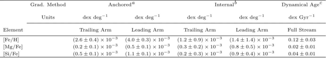
Using 3D positions and kinematics of stars relative to the Sagittarius (Sgr) orbital plane and angular momentum, we identify 166 Sgr stream members observed by the Apache Point Observatory Galactic Evolution Experiment (APOGEE) that also haveGaiaDR2 astrometry. This sample of 63/103 stars in the Sgr trailing/leading arm are combined with an APOGEE sample of 710 members of the Sgr dwarf spheroidal core (385 of them newly presented here) to establish differences of 0.6 dex in median metallicity and 0.1 dex in [α/Fe] between our Sgr core and dynamically older stream samples. Mild chemical gradients are found internally along each arm, but these steepen when anchored by core stars.

crh7gs@virginia.edu

arXiv:1912.06707v1 [astro-ph.GA] 13 Dec 2019

With a model of Sgr tidal disruption providing estimated dynamical ages (i.e., stripping times) for each stream star, we find a mean metallicity gradient of 0.12±0.03 dex/Gyr for stars stripped from Sgr over time. For the first time, an [α/Fe] gradient is also measured within the stream, at 0.02±0.01 dex/Gyr using magnesium abundances and 0.04±0.01 dex/Gyr using silicon, which imply that the Sgr progenitor had significant radial abundance gradients. We discuss the magnitude of those inferred gradients and their implication for the nature of the Sgr progenitor within the context of the current family of Milky Way satellite galaxies, and suggest that more sophisticated Sgr models are needed to properly interpret the growing chemodynamical detail we have on the Sgr system.

Keywords: Galaxy: structure−Galaxy: evolution−Galaxy: halo−stars: abundances −galaxies:

individual: Sagittarius dwarf spheroidal 1. INTRODUCTION

The Sagittarius (Sgr) dwarf spheroidal (dSph) galaxy and its tidal stream provide a nearby and vivid example of a tidally disrupting dwarf galaxy (Ibata et al. 1994;

Majewski et al. 2003) and the hierarchical growth of large galaxies through minor mergers. Because Sgr is in a quite advanced stage of tidal stripping, yet its stars are not yet fully mixed with those of the Milky Way (MW), the system has become a remarkably versatile tool for exploring a great variety of astrophysical problems.

Numerous studies have exploited the extensive tidal debris structure as a sensitive probe of the MW, its dark matter content, and its dynamics. For example, because Sgr’s tidal arms wrap through a large extent of the MW halo and trace the past and future orbit of the core, they can constrain the 3D shape of the MW’s dark matter halo (Helmi 2004; Johnston et al. 2005; Law et al. 2005; Law & Majewski 2010;Deg, & Widrow 2013;

Ibata et al. 2013;Vera-Ciro, & Helmi 2013). Moreover, the alignment of Sgr’s orbit is nearly perpendicular to the MW disk and crosses the disk midplane relatively near the Sun-Galactic Center axis; this fortuitous con- figuration means that the solar rotational velocity can also be gauged directly via the reflex solar motion im- printed in the velocities/proper motions of stars in the stream (Majewski et al. 2006; Law & Majewski 2010;

Carlin et al. 2012;Hayes et al. 2018). Sgr has also been identified as a possible culprit for dynamical perturba- tions observed in the MW disk, and as such provides a case study on the potential effects of minor mergers on the evolution of the stellar and HI disks (Ibata & Ra- zoumov 1998; G´omez et al. 2013; Laporte et al. 2018, 2019).

Obviously, the Sgr system also lends uniquely acces- sible and detailed insights into the tidal disruption and

∗NSF Astronomy and Astrophysics Postdoctoral Fellow

†Hubble Fellow

Carnegie-Princeton Fellow

dynamical evolution of dwarf galaxy satellites. This in- cludes not only clues into potential morphological and dynamical changes in dwarf galaxies induced by the en- counters with larger galaxies like the MW ( Lokas et al.

2010; Pe˜narrubia et al. 2010, 2011; Frinchaboy et al.

2012; Lokas et al. 2012;Majewski et al. 2013), but also effects on their star formation histories and the chemical evolution of their stellar populations. The latter have clearly been shaped by the interplay between episodic star formation incited by gravitational shocking at or- bital pericenter and the stripping of gas (Siegel et al.

2007;Tepper-Garc´ıa & Bland-Hawthorn 2018).

A particularly important lesson learned from studies of the Sgr system is that any assessment of the chem- ical and star formation histories and distribution func- tions of Sgr or another tidally disrupted system will be incomplete and biased without properly accounting for the stellar populations lost via tidal stripping (Chou et al. 2010; Carlin et al. 2018, ; see also earlier discussions of this phenomenon inMajewski et al. 2002;Mu˜noz et al. 2006). This is because tidal stripping preferentially acts on the least bound stars in a dwarf, and those stars tend to be older and less chemically evolved stars in the system.

The discovery of large mean metallicity differences at the level of ∆[Fe/H] ∼0.4-0.6 dex between samples of stars in the Sgr core and the (lower metallicity) Sgr stream (Chou et al. 2007;Monaco et al. 2007) provided early suggestions of the possible metallicity gradients along the Sgr stream. If such chemical gradients do indeed exist along the Sgr stream, they may be the preserved remnants of chemical gradients that existed within the Sgr progenitor galaxy.

N-body modeling of Sgr’s tidal stripping was imple- mented by Law & Majewski (2010, hereafter LM10), who used a prescription for assigning metallicities to model particles based on their initial energy in the bound progenitor, which naturally yielded a radial gra- dient in mean metallicity in the simulated dwarf. Based on this modeling,LM10found that the observed metal-

licity differences between stream and core implied a mean radial metallicity variation as large as 2.0 dex be- fore Sgr’s tidal disruption, exceeding that seen in any other dwarf galaxy.

Since these first identifications of significant metallic- ity differences between the Sgr stream and core, further studies have measured the metallicity of Sgr stream stars and reported metallicity gradients (Keller et al. 2010;

Carlin et al. 2012; Shi et al. 2012; Hyde et al. 2015) along the Sgr stream. However, the sampling and mea- surement of gradients was not consistent across studies, which complicates their comparison. Specifically, some authors report metallicity gradients from the Sgr core through each tidal arm (such that the high end of the gradient is anchored by the metallicity of the core) and find metallicity gradients of about 2.4-2.7 ×10⁻³ dex deg⁻¹along the trailing arm (Keller et al. 2010;Hyde et al. 2015). Other studies measure only the internal metal- licity gradients within each arm (excluding the metallic- ity of the Sgr dSph core), which produces much flatter gradients, around 1.4-1.8 ×10⁻³ dex deg⁻¹ along the trailing arm and about 1.5×10⁻³ dex deg⁻¹ along the leading arm (Carlin et al. 2012;Shi et al. 2012).

Because a large fraction (75% at high latitudes) of the MW halo M giants belong to the Sgr stream (Majewski et al. 2003), some studies have employed a color selection to exclusively study the relatively metal-rich M giants in the stream, since they are subject to less contamination than samples of the more common K giants (Chou et al.

2007;Monaco et al. 2007;Keller et al. 2010;Carlin et al.

2018). However, M giants are only produced by higher metallicity populations, so these samples would have an implicit metallicity bias, and could skew some of these past measurements of metallicity gradients.

Because of the observational demands required by high-resolution spectroscopy, few detailed chemical abundance studies of stream stars have been performed, and only measured abundances for relatively small sam- ples (Monaco et al. 2007; Chou et al. 2010; Keller et al. 2010; Carlin et al. 2018). However, such studies have attempted to explore theα-element abundances of Sgr stream stars, and typically report similarα-element abundance levels to stars in the Sgr coreMonaco et al.

(2007);Chou et al.(2010);Carlin et al.(2018), or equiv- alently suggest no significantα-element gradients along the stream (Keller et al. 2010).

The Apache Point Observatory Galactic Evolution Experiment (APOGEE; Majewski et al. 2017) provides a unique opportunity to study the detailed chemistry of the Sgr stream. APOGEE is a high-resolution (R ∼ 22,500),H-band (1.5-1.7µm) spectroscopic survey that primarily targets red giant stars and samples a relatively

large area of the sky. While the APOGEE survey im- poses a blue color limit to prioritize observations of red giants and minimize contamination from warmer main sequence dwarfs, this limit, (J −K)0 ≥ 0.3 in halo fields (|b| & 16^◦, where most of the Sgr stream lies) and (J−K)0≥0.5 otherwise, is still liberal enough to provide relatively unbiased metallicity coverage for red giant branch stars (RGB; Zasowski et al. 2013, 2017).

In addition, the dual-hemisphere coverage of APOGEE- 2 allows us to sample nearly continuously along large sections of both arms of the Sgr stream.

Observations of Sgr dSph core members were first re- ported in APOGEE by Majewski et al. (2013) using the Sloan Digital Sky Survey (SDSS) Data Release 12 (DR12Alam et al. 2015), and the membership was ex- panded by Hasselquist et al. (2017) using SDSS DR13 (Albareti et al. 2017; Holtzman et al. 2018), both tak- ing advantage of the intentional APOGEE targeting of the Sgr core. While a few APOGEE fields were placed intentionally along the Sgr stream, Hasselquist et al.

(2019) demonstrated that both the trailing and lead- ing arm of the Sgr stream are relatively well-sampled serendipitously by the random targeting employed by the APOGEE survey.

Hasselquist et al. (2019) used chemical tagging to identify 35 relatively metal-rich, [Fe/H] & −1.2, Sgr stream stars in the APOGEE data presented in SDSS DR14 (Abolfathi et al. 2018; Holtzman et al. 2018), which only included APOGEE data in the Northern Hemisphere. However, the chemical tagging method that was used to identify these Sgr stars is limited to these higher metallicities, because it relies on the fact that the chemical abundance profile of Sgr is distinct from the MW at these metallicities (Hasselquist et al.

2017,2019).

At lower metallicities, the chemical abundance profile of Sgr begins to merge with that of the accreted MW halo (Hayes et al. 2018; Hasselquist et al. 2019), so to push to lower metallicities we must use other means to identify Sgr members. Fortunately, the Sgr system, in- cluding the Sgr stream, possesses a relatively unique or- bit that enables Sgr stream members to be readily iden- tified kinematically from surveys of the MW. The Sgr stream is also sufficiently close that Gaia DR2 proper motions (Gaia Collaboration et al. 2018), APOGEE ra- dial velocities, and spectrophotometric distances can be measured to such a precision that complete 6-D phase space information can be obtained for large samples of candidate stars. Because a selection of the Sgr stream candidates from the 6-D phase space distribution of APOGEE-observed stars is relatively free from metal- licity bias, one can reliably measure chemical gradients

along the Sgr stream from the identified stream mem- bers.

In this work we perform such a selection of Sgr stream stars based on their 3D positions and velocities rela- tive to the Sgr orbital plane. We also exploit the fact that APOGEE-2 is now operating in both the Northern and Southern Hemispheres, so that, with the dual hemi- sphere APOGEE data reported in SDSS DR16 (Ahu- mada et al. 2020;J¨onsson et al. in prep.), we can obtain a more complete coverage of both the leading and trail- ing arms of the the Sgr stream. With a relatively large sample of Sgr stream members, and the precise multi- element APOGEE abundances, we can also begin prob- ing gradients in chemical abundance ratios along the Sgr stream as well as metallicity gradients.

Section 2 provides an overview of the data and quality restrictions we employ for our study. Section 3 describes the selection criteria applied for identifying Sgr stream stars based on their 3D positions and kinematics within a Galactocentric coordinate system defined by the Sgr orbital plane. Using the high precision bulk metallici- ties and chemical abundances that APOGEE measures, in Section 4 we discuss the chemical differences found between the Sgr stream and core in Section 4.1, our as- sessment of metallicity gradients along the Sgr stream in Section 4.2, the first measurements of non-zero α- element abundance gradients along the stream in Sec- tion 4.3, and, through the use of an N-body simulation, we collate the data from the two arms to understand the chemical gradients as a function of dynamical age or stripping time in the Sgr stream in Section 4.4. Section 5 discusses the implications that the measured chemical differences and gradients along the stream have for the chemical structure of the progenitor Sgr galaxy. Finally, in Section 6 we present our main conclusions.

2. DATA

The data in this paper come primarily from the APOGEE survey (Majewski et al. 2017) and its succes- sor APOGEE-2. We use the APOGEE data in SDSS- IV DR16 (Blanton et al. 2017; Ahumada et al. 2020;

J¨onsson et al. in prep.) that will be made publicly available in December 2019. This data release includes data taken from both the Northern and Southern Hemi- spheres using the APOGEE spectrographs (Wilson et al. 2019) on the SDSS 2.5-m (Gunn et al. 2006) and the 2.5-m du Pont (Bowen & Vaughan 1973) telescopes re- spectively. The targeting procedure for APOGEE is pre- sented inZasowski et al.(2013,2017) andBeaton et al.

(in prep.), and details of the data reduction pipeline for APOGEE can be found inNidever et al.(2015). Stellar parameters and chemical abundances are derived from

the APOGEE Stellar Parameter and Chemical Abun- dance Pipeline (ASPCAP; Garc´ıa P´erez et al. 2016), based on theferre¹ code, through a similar procedure as in SDSS DR14/15. For SDSS DR16, ASPCAP has now been updated to use a grid of only MARCS stel- lar atmospheres (Gustafsson et al. 2008), rather than Kurucz (Kurucz 1979; J¨onsson et al. in prep.), and us- ing a new H-band line list from Smith et al.(in prep.) that updates the earlier APOGEE line list presented in Shetrone et al.(2015), all of which are used to generate a grid of synthetic spectra (Zamora et al. 2015).

From the full APOGEE sample, we remove stars flagged² as having the starflags: bad pixels, very bright neighbor, or low snrset, or any stars with poorly determined stellar parameters, as may be indicated by the aspcapflags: rotation warn or star bad. Since we do not expect to detect dwarf stars in APOGEE at the distance of the Sgr stream, we limit our analysis to giant stars by selecting stars with calibrated logg <4. In addition we only analyze stars with low velocity uncertainty, Verr ≤0.2 km s⁻¹, and, when considering chemical abundances in Sections 4 and further sections, we require stars to have S/N>70 per pixel spectra to remove stars with lower quality spectra and consequently less reliable ASPCAP-derived stellar parameters and chemical abundances. We also restrict our chemical analysis in Section 4 and beyond to stars with effective temperatures warmer than 3700 K, where APOGEE stellar parameters and chemical abundances are reliably and consistently determined (for more de- tails on the APOGEE DR16 data quality seeJ¨onsson et al. in prep.).

Since we are interested in kinematically identifying distant Sgr Stream stars, we also remove stars that are associated with known globular clusters based on spa- tial and radial velocity cuts (except the globular cluster M54 that lies in the Sgr dSph), which helps reduce con- tamination from globular clusters on similar orbits to Sgr. While some globular clusters may be associated with Sgr, and therefore participated in its overall evo- lution (Da Costa & Armandroff 1995;Ibata et al. 1995;

Dinescu et al. 2000;Bellazzini et al. 2003; Law, & Ma- jewski 2010b), we want to understand the chemical evo- lution of the main Sgr progenitor, and in any case, glob- ular clusters are contaminated with peculiar chemical pollution differentiating the first generation stars from the second generations that appear to exhibit chemistry

1https://github.com/callendeprieto/ferre

2A description of these flags can be found in the online SDSS DR15 bitmask documentation (http://www.sdss.org/dr15/algorithms/

bitmasks/)

unique from the rest of the Galaxy. We additionally re- move the APOGEE fields centered on or near the Large and Small Magellanic Clouds (MCs), which are (unsur- prisingly) dominated by the heavy sampling of MC stars and are unlikely to contain Sgr stream stars anyway, be- cause these fields do not lie along the Sgr stream.

We supplement the APOGEE data with proper mo- tions from Gaia DR2 (Gaia Collaboration et al. 2018) and with spectrophotometric distances calculated with the Bayesian distance calculatorStarHorse(Santiago et al. 2016;Queiroz et al. 2018) using multiple photomet- ric bands, the APOGEE DR16 stellar parameters, and, when possible, parallax priors fromGaiaDR2 (Queiroz et al. in prep.). We use the APOGEE DR16StarHorse distances (Queiroz et al. in prep.) rather than those that are calculated more purely from parallaxes, such as the Bailer-Jones et al.(2018) distances, because, as of Gaia DR2, these astrometric distances are primarily driven by priors for sources beyond heliocentric distances of 5 kpc (where the parallax uncertainties become too large), and therefore have large uncertainties (>20%).

Such large uncertainties are problematic for identi- fying Sgr stream stars given that, at the closest point to the sun, the Sgr stream is still beyond 10 kpc away (Majewski et al. 2003; Koposov et al. 2012), and mo- tivate using spectrophotometric distances, such as the APOGEE DR16 StarHorsedistances, which maintain an internal precision of ∼10%, even at distances much larger than 10 kpc. While other spectrophotometric dis- tance catalogs are publicly available, we have chosen the APOGEE DR16StarHorse distance catalog presented inQueiroz et al.(in prep.) because these distances have been calculated using the new, updated APOGEE DR16 stellar parameters and are available for almost all stars in APOGEE DR16, including the∼170,000 stars added since the last public data release. Thus, the StarHorse distance catalog covers our APOGEE sample more com- pletely and self-consistently than other publicly avail- able spectrophotometric distance catalogs that are lim- ited to smaller APOGEE data releases, older versions of the ASPCAP-derived stellar parameters, or stellar parameters derived from other, unassociated data sets (e.g., Wang et al. 2016; Sanders, & Das 2018; Hogg et al. 2019).

A small fraction of the stars in our sample have StarHorse distances that are flagged with poor solu- tions (due to having poor or high infrared extinction, or too few stellar models from which to estimate dis- tances), so we excise these stars from our sample. Out of the 437,485 unique APOGEE targets, 256,275 are gi- ants that satisfy our spectroscopic quality restrictions, and from which we remove: 2,581 giants because they

are identified as globular cluster members, 8,977 giants that fall in fields around the MCs, and finally 2,595 re- maining stars with flaggedStarHorsedistances. After applying these quality cuts, our cross-matched sample of APOGEE observed stars with Gaia measurements andStarHorsedistances amounts to 242,122 giants hav- ing measured stellar parameters, chemical abundances, radial velocities, proper motions, and distances, from which we identify Sgr stream candidates.

3. TRACING THE SGR STREAM 3.1. Selecting Sgr Stream Candidates

We want to identify Sgr stream members from APOGEE based on their location and kinematics, and now, with the high precision proper motions available fromGaia DR2 and spectrophotometric distances from StarHorsethat are relatively precise even out to large distances, we can find members using full 3D spatial velocities. We calculate the Galactocentric coordinates for our cleaned and cross-matched APOGEE sample, using StarHorse distances assuming RGC, = 8.122 kpc (Gravity Collaboration et al. 2018). We then in- clude the APOGEE radial velocities and theGaiaDR2 proper motions to calculate the 3D heliocentric spatial velocities of these stars using the prescription inJohn- son & Soderblom(1987), and convert these to Galacto- centric space velocities assuming a total solar motion of (V_r, V_φ V_z) = (14,253,7) km s⁻¹ in the right-handed velocity notation (Sch¨onrich et al. 2010;Sch¨onrich 2012;

Hayes et al. 2018).

Because the Sgr stream arches across the sky in a near great circle, it has been historically possible to define relatively precisely the orbital plane of the Sgr system without kinematics (Majewski et al. 2003). While we can use the Galactocentric positions and velocities of stars within our sample to identify Sgr stream stars by their general net motion, we can make an even more careful selection of these members by considering their motion with respect to the very well-defined Sgr orbital plane. Therefore, we take the Galactocentric positions and velocities that we have calculated and rotate them into the Sgr orbital plane according to the transforma- tions described inMajewski et al.(2003, here we use the definition of the Galactocentric Sgr coordinates where ΛGC= 0 is set at the Galactic midplane, sometimes re- ferred to as the Λ4coordinate system).³ This produces a set of position and velocity coordinates (which are most usefully expressed in Cartesian or cylindrical forms) rel-

3See also the publicly available code that can be used to per- form transformations into the Sgr coordinate systems athttp:

//faculty.virginia.edu/srm4n/Sgr/code.html.

ative to the Sgr orbital plane, rather than to the plane of the Galaxy, but still centered on the Galactic center.

Rather than using a model to predict the location and kinematics expected of Sgr stream stars, we want to use a data-driven selection of these stars, and can then com- pare them to models as further verification of their mem- bership status. To first order, we can expect that Sgr stream stars should have conserved their orbital angular momentum, and to the accuracy of our data, the orbital angular momentum of Sgr stream stars within our sam- ple should be the same as the orbital angular momentum of known members of the Sgr dSph. APOGEE has ob- served a considerable number of stars in the Sgr core (Majewski et al. 2013; Hasselquist et al. 2017), which we can use to establish the range of orbital angular mo- menta of the core, and use that range to select stream candidates.

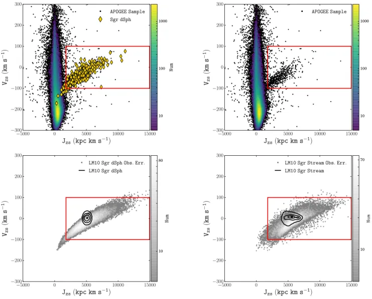
Because the Sgr system is relatively well confined to the nominal Sgr orbital plane (modulo possible preces- sion of the orbital plane; Law et al. 2005; LM10), we should expect that stars in the Stream and the dSph to have conserved the same angular momentum (within our uncertainties), and should not have large velocities perpendicular to the orbital plane. This concept serves as the main selection criteria we employ to select stars in the Sgr dSph and Stream system. We therefore compute the specific angular momentum of stars in our sample along the z-direction of our Galactocentric Sgr coordi- nates, Jzs =RGC,s×Vφ,s (i.e., the angular momentum perpendicular to the Sgr orbital plane), and in Figure1 show the angular momentum of stars in our sample in this direction versus their velocity perpendicular to the Sgr orbital plane (V_z,s). Because the Sgr orbital plane is nearly perpendicular to the Galactic plane, most of the APOGEE sample (which is dominated by stars in the disk of the MW near the sun) are rotating with the Galactic disk out of the Sgr orbital plane in the direction of−Vz,s, and typically have low velocities perpendicular to or radially within the disk of the MW, so they have low velocities in the Sgr orbital plane, and thus a low angular momentum along the direction perpendicular to the Sgr orbital plane.

Known Sgr dSph members from Hasselquist et al.

(2017), however, show a relatively largeJz,s, as seen in Figure1, albeit with a wide spread due to distance un- certainties, but a relatively small velocity perpendicular to the Sgr orbital plane, and identify a range in phase space where we would expect Sgr stream stars to lie. The correlation between Jz,s and Vz,s in the Sgr core is an artifact of distance uncertainties inflating/deflating the velocity and angular momenta of core members, because theVz,sandVφ,sin the direction of the Sgr core predomi-

nantly come from proper motions, which are nearly con- stant across the Sgr core, so a spread in distances will produce a correlated spread in Vz,s and Vφ,s, and thus between theVz,sandJz,sin the core.

The bottom panels of Figure 1 show particles from the LM10model in the Jz,s−Vz,s plane, and compare their distribution in this projection of phase space when measured perfectly (i.e., with no distance errors) ver- sus how they spread when measured with random 10%

distance errors, typical of those in our sample. These simulated observations demonstrate the affects of dis- tance errors alone, yet appear to mimic the observed correlations seen in our distribution of Sgr dSph mem- bers. The simulations also illustrate that the stream will, as expected, cover a similar region of this param- eter space as the Sgr dSph core, and further justifies that the range of Z_sangular momenta and velocities of known Sgr dSph members can indicate where we may find Sgr stream candidates.

To reduce MW contamination, we use a relatively con- servative cut in Jz,s to select Sgr system candidates, selecting stars with Jz,s > 1800 kpc km s⁻¹, and re- move stars with velocities perpendicular to the Sgr or- bital plane |Vz,s| > 100 km s⁻¹ to isolate only those stars with a low velocity perpendicular to the Sgr or- bital plane. To clean out stars that deviate too far from the Sgr orbital plane, we additionally remove any stars that are at Sgr plane latitudes |BGC| >20^◦. We also remove stars that are within a heliocentric distance of 10 kpc, since the Sgr Stream is known to not come this close to the Sun’s position in the MW (Majewski et al.

2003;Belokurov et al. 2014;Hernitschek et al. 2017).

3.2. Removing Halo Contamination

This initial selection of Sgr stream candidates is shown in Figure2. The Sgr stream stands out prominently, as the arc of leading arm stars above the disk,Ys<0, and the curve of trailing arm stars below the disk, Y_s >0, but is still contaminated by what appear to be remaining halo stars, seen as stars with peculiar velocity vectors, which we want to remove. This potential halo contam- ination comes in two flavors: (1) stars moving in di- rections inconsistent with the photometrically implied motion of the Sgr stream (i.e., stars that move nearly perpendicular to the direction of the stream at their lo- cation), and (2) stars that are moving in the correct direction, but are still too close to the Sun to be consis- tent with the location of the stream (despite attempting to remove such contamination by removing stars within 10 kpc of the Sun), even when accounting for distance uncertainties.

−5000 0 5000 10000 15000

Jzs(kpc km s⁻¹)

−300

−200

−100 0 100 200 300

Vzs(kms−1)

APOGEE Sample Sgr dSph

10 100 1000

Num

−5000 0 5000 10000 15000

Jzs(kpc km s⁻¹)

−300

−200

−100 0 100 200 300

Vzs(kms−1)

APOGEE Sample

10 100 1000

Num

−5000 0 5000 10000 15000

Jzs(kpc km s⁻¹)

−300

−200

−100 0 100 200 300

Vzs(kms−1)

LM10 Sgr dSph Obs.Err.

LM10 Sgr dSph

10 80

Num

−5000 0 5000 10000 15000

Jzs(kpc km s⁻¹)

−300

−200

−100 0 100 200 300

Vzs(kms−1)

LM10 Sgr Stream Obs.Err.

LM10 Sgr Stream

10 70

Num

Figure 1. Velocity of stars (top panels) orLM10star particles (bottom panels) perpendicular to the Sgr orbital plane,Vz,svs.

their angular momentum about the axis perpendicular to the Sgr orbital plane,Jz,s. (Top panels) APOGEE observed stars with GaiaDR2 proper motions and StarHorsedistances are shown (black points, and 2D histogram for densely populated regions of this space), and the known members of the Sgr core in APOGEE fromMajewski et al.(2013) andHasselquist et al.(2017) are highlighted (gold diamonds in the left panel only). The red box illustrates our initial selection of Sgr stream candidates in this parameter space, and those candidates are shown more clearly in the right panel. (Bottom left panel) The distribution ofLM10Sgr dSph particles (i.e., particles that are still bound in the model) in this projection of phase space (black contours, containing 95%, 68%, 32%, and 5% of the particles, from the outside-in), are shown over top of simulated observations of these particles when they are measured with random 10% distance errors (gray points and 2D grayscale histogram), typical of our StarHorsedistance uncertainties. (Bottom right panel) Same as the bottom left panel, but now illustrating the effect of 10%

distance uncertainties on the distribution of LM10Sgr stream particles (particles that became unbound within the last three Sgr pericenter passages).

Most of the contamination appears to be above the MW disk (Ys<0), and is particularly noticeable atYs∼

−10 kpc, where there is a spread in theXs distribution of our Sgr stream candidates of about 30 kpc, ranging from Xs∼ −30 kpc to 0 kpc. Because the distance to the stream is known to be ∼ 20 kpc or more in this area of the sky (Belokurov et al. 2014; Hernitschek et al. 2017) the spread of stars between Xs ∼ −15 to 5

kpc and Y_s ∼ −20 to −10 kpc are likely to be halo contamination, because they are too close to the Sun.

While some of these stars have motions that are in the correct direction to be consistent with the Sgr stream, even if their StarHorse distances were un- derestimated, placing them at the distance of the Sgr stream, but keeping their observed proper motions and radial velocities would inflate their space velocities too

−80 −60 −40 −20 0 20 40 Xs(kpc)

−60

−40

−20

0

20

40 Ys(kpc)

+

Sgr Cand,200 km s⁻¹ Sgr dSph,200 km s⁻¹

−60 −40 −20 0 20 40 60

Zs(kpc)

−60

−40

−20

0

20

40 Ys(kpc)

Sgr Cand,200 km s⁻¹ Sgr dSph,200 km s⁻¹

Figure 2. Velocity plot of the Galactocentric distribution of Sgr stream candidates selected as described in Section3.1(black arrows), along with known members of the Sgr core (gold arrows; Hasselquist et al. 2017), as projected onto the Sgr orbital plane of Ys vs. Xs and the Galactocentric Sgr Ys vs. Zs plane. The median 1σ uncertainty on these positions is shown bottom left-hand corner (the orientation of these uncertainties is dominated by the Sgr dSph core and the typical orientation of uncertainties for a given star will have maximal uncertainty parallel to the sun-star direction). The arrows depict the direction and magnitude of the velocity of these stars in this plane. For reference, the location of the sun and the Galactic center are marked (as anand + symbol respectively). While there appears to be some minor contamination from halo field stars, the bulk of this sample of Sgr stream candidates appear to follow the direction of the Sgr stream with coherent change in the magnitude of velocities along the stream as orbits reach apocenter or pericenter (both in magnitude and direction).

high for them to be consistent with the rest of the Sgr stream candidates in our sample. We therefore remove the stars that are too close to the Sun, and are only left with potential halo contamination that is not moving in the correct direction of the stream.

The dominant contributors of stream stars above and below the MW disk midplane are the leading and trailing arms respectively. Therefore, we would expect stream members to be moving along the direction of the re- spective arms when we consider stars above and below the disk. Because we imposed an angular momentum requirement to select our Sgr stream candidates, the stars moving in directions that are inconsistent with the stream around them are primarily stars moving perpen- dicular to the bulk of our candidate sample. However, the arms of the Sgr stream are thought to cross each other, both above and below the disk, and this cross- ing could yield a smaller set of candidates from the less dense arm in that Galactic hemisphere that move per- pendicular to the stars from the more densely populated arm. We want to consider whether we are actually iden- tifying any such stars, or if the stars with peculiar mo- tions are instead contamination from the MW halo.

In the Northern Galactic Hemisphere, above the MW disk (Ys<0), the leading arm is the more densely pop- ulated arm of the Sgr stream, and in the left panel of Figure2 we do see some stars that are moving perpen- dicular to the remainder of our stream candidates in this region. The LM10 model predicts that the trail- ing arm should cross the leading arm above the disk at (Xs, Ys) ∼ (−20,−20) kpc. However, the position of this crossing in the LM10 model is very sensitive to the shape (and possible time-variance) of the MW gravitational potential, and recent studies suggest that the trailing arm instead crosses the leading arm at a point much further above the plane (∼50 kpc), or may pass over it entirely (Hernitschek et al. 2017;Sesar et al.

2017). This means that above the MW disk the trail- ing arm lies in regions where the density of APOGEE targets (and stream candidates) is much lower, and the few stars we see moving perpendicular to the rest of our sample are likely halo contamination.

The crossing of the leading and trailing arms below the MW disk has remained somewhat elusive, with only a few studies suggesting they have observed a few stars in the leading arm below the disk (Majewski et al. 2004;

Chou et al. 2007;Carballo-Bello et al. 2017), but there is still no convincing trace of the extent of the leading arm after plunges through the crowded and dust extin- guished MW plane. We do find four stream candidates that are moving perpendicular to the bulk of our sam- ple below the disk with roughly the correct position and velocity to be in the leading arm, but given the low num- ber of these stars it is hard to confidently associate them with the Sgr stream. To provide a conservative sample of Sgr stream members, we will not include these can- didates in our final sample, but we do note that they may bebona fideSgr Stream members belonging to the leading arm.

To quantitatively remove the aforementioned halo contamination moving in incorrect directions to be members of the Sgr stream, and to remove stars that we cannot confidently associate with the Sgr stream, we assess the candidate stream members’ orbital veloc- ity position angle,φvel,s≡arctan(−Vx,s/−Vy,s), in the Sgr orbital plane. This orbital velocity position angle is defined to be zero in the −Ys direction and increasing through the−Xsdirection, such that as Sgr moves along its orbit it has an increasing orbital velocity position an- gle. If the Sgr system were on a perfectly circular orbit, this orbital velocity position angle would be expected to change linearly with Sgr Stream longitude as measured from the Galactic Center, Λ_GC; however, because the Sgr orbit is somewhat eccentric, this relation will vary from linearity.

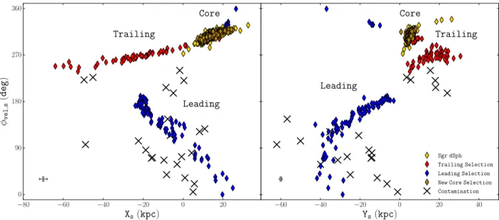
In Figure3we show the orbital velocity position angle, φvel,s, of the Sgr core members and Sgr stream candi- dates as a function of theirXsandYsposition in the Sgr orbital plane. Here the leading and trailing arms stand out differently; the leading arm shows a linear distribu- tion in φvel,s−Ys at Ys .0 kpc that becomes a more tenuous distribution around Y_s ∼ 40 kpc, whereas the trailing arm has a very tight and nearly linear distribu- tion in φvel,s−Xs, but is clumped in the φvel,s−Ys. To remove potential halo contamination, we remove any of the Sgr stream candidates that deviate significantly from the stream loci in one of these two planes, and mark which stars have been removed.

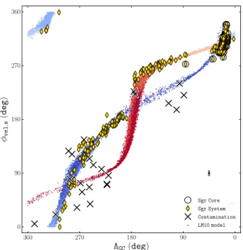
These Sgr stream member selections on orbital ve- locity position angle have been applied to remove the stars most inconsistent with our simple hypothesis that the stream should be dynamically coherent, but we can also compare this final selection of stars with theLM10 model to further justify our criteria. In Figure 4 we compare theφvel,sas a function of Sgr longitude as seen from the Galactic Center, ΛGC, for both our selected sample of Sgr stream stars and the likely MW halo con-

tamination as identified above to predictions from the LM10model.

This comparison shows that the final Sgr stream sam- ple is not only very tightly coherent in its distribution, but that it closely follows the predictions of the model, which is reassuring given that this requires a precise combination of the observed distances, proper motions, and radial velocities in the data. Additionally we see that the stars labeled as likely contamination, by and large, deviate much more significantly from the model.

While there are a few contaminant stars that do line up with the model, they do so along parts of the stream that are poorly modeled/constrained or they physically lie in regions of the halo where the stream (and the rest of our sample) does not pass.

Our final selection identifies 518 new members of the Sgr system in the APOGEE survey, including 133 new Sgr stream stars and 385 new Sgr dSph core stars, and we recover 33 of the 35 metal-rich APOGEE Sgr Stream members found by Hasselquist et al. (2019) through chemical tagging. The advantage here is that our kine- matic selection now allows us to push below the [Fe/H]

∼ −1.2 metallicity that was the limit for the chemi- cal tagging, below which the chemical abundance pro- file of Sgr begins to blend with that of the MW halo (Hasselquist et al. 2019). The two remaining stream stars thatHasselquist et al.(2019) found were not recov- ered because they lack distances measurements in this APOGEE data release.

To constitute a more complete census of the Sgr sys- tem that we analyze throughout the rest of this paper, we combine this sample of new members with (1) the 325 known Sgr dSph stars fromHasselquist et al.(2017) that pass our spectroscopic and distance requirements (299 of which we recover through our Sgr selection; the remaining 26 are excluded by ourJ_z,s−V_z,scuts to avoid MW contamination, as seen in Figure1), and (2) the 33 Sgr stream stars fromHasselquist et al.(2019) that we recover. This gives a total sample of 876 APOGEE ob- served stars in the Sgr system, the largest sample of Sgr stars with high-resolution spectra to date. Of the 166 Sgr Stream stars, 103 of them are in the leading arm, and 63 are in the trailing arm.

The distribution of this full Sgr sample throughout the Galactocentric Sgr coordinate system is shown in Figure 5overlying the LM10 model of the Sgr Stream pulled off of the main body within the past three pericenter pas- sages (P_col≤3), with arrows illustrating the magnitude and direction of each star’s velocity projected onto these planes. Despite not being selected in accordance with the LM10 model, we can see that on average, our Sgr Stream sample aligns well with theLM10model in terms

−80 −60 −40 −20 0 20

Xs(kpc)

0 90 180 270 360

φvel,s(deg)

Trailing

Leading Core

−60 −40 −20 0 20 40

Ys(kpc)

Trailing

Leading

Core

Sgr dSph Trailing Selection Leading Selection New Core Selection Contamination

Figure 3. Orbital velocity position angle,φvel,s, vs. Xs(left panel), and vs. Ys(right panel) of the Sgr stream candidates that have been identified as likely contamination (black crosses), those that are likely real members of the trailing arm and leading arm (red and blue diamonds respectively), new core members (dark yellow diamonds), and known Sgr dSph members (as defined in Figure 1). The median 1σ uncertainties on these positions and angles are shown in the bottom left-hand corner, but note that, as in Figure2, the magnitude of theXs andYs uncertainties change slightly depending on location and these error bars are most representative of stars located in the Sgr core. Stars identified as likely halo contamination move nearly perpendicular to the leading arm at a location where the trailing arm is now established not to cross (φvel,s∼ ±90^◦from the overdensity of likely Sgr stream members at a givenXs orYsposition) and stand away from the Sgr stream locus in one of these two planes, or lie in regions where the leading arm is thought to pass below the MW disk, but the density of Sgr stream stars is low and has not been clearly traced.

of shape and distance for the most part, however, there are two differences: (1) The width of the Sgr stream in our observed sample appears to be slightly inflated in some places due to distance uncertainties that spread stars along the radial direction from the sun (although these distances seem to be precise enough to differenti- ate the narrower width of the leading arm and against wider trailing arm at their points nearest the sun), and (2) there appears to be a difference in the distance scale between the observations and theLM10 model, partic- ularly at the Sgr dSph core and at the apocenter of the leading arm, such that the observed distances are mea- sured closer to the Sun on average.

The median distance to the Sgr core in our sample is about 23 kpc, with a dispersion ofσ = 4 kpc, whereas past studies find slightly larger distances, ranging from 24-28 kpc (Monaco et al. 2004; Siegel et al. 2007; Mc- Donald et al. 2013; Hernitschek et al. 2019), although we note that our median distance to the Sgr core is still within about 1σ of these previously measured dis- tances. One possible source of our smaller distances to the Sgr core, may be the bulge priors used in calcu- lating StarHorse distances. To account for the higher density of stars in the Galactic bulge when calculating

StarHorsedistances, Queiroz et al.(2018) incorporate a prior for stars in the direction of the Galactic Center to lie at distances that place them in the bulge. Because the Sgr dSph core lies opposite the bulge from the Sun, it lies in a part of the sky where this prior is relevant for MW stars, but it may be skewing the distances of Sgr stars to smaller values.

However, we can see that the distances to other parts of the stream are also skewed to smaller values than in theLM10model (by∼15−20%). This may suggest that the Queiroz et al.(2018) values are systematically un- derestimated at these large distances, or that theLM10 model overestimates the distances to the Sgr system (for which there is some evidence in comparison with the distribution of Sgr stream RR Lyrae, which find slightly closer distances for the apocenter of the leading arm Hernitschek et al. 2017). Regardless, neither possibility should have serious impact on the results that follow, be- cause we use the distance independent heliocentric Sgr longitudinal coordinate system for the remaining analy- sis.

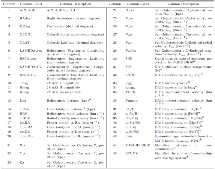
Our final sample of Sgr stars (core and stream) are given in Table 1, along with their positions, kinemat- ics, stellar parameters and chemical abundances (for

0 90

180 270

360

Λ_GC(deg)

0 90 180 270 360

φvel,s(deg)

Sgr Core Sgr System Contamination LM10 model

Figure 4. Orbital velocity position angle,φvel,s, vs. Galac- tocentric Sgr longitude, ΛGC for the final sample of stars selected to be members of the Sgr system (gold diamonds, with the previously known Sgr dSph core members circled in black), and the Sgr stream candidates that were identi- fied as likely halo contamination (black crosses), compared to particles from theLM10Sgr model (colored points), with the median uncertainty on these angles shown as the error- bar to the lower right (above the legend). The LM10 model points have been colored to identify the leading (blue) and trailing (red) arms with darker saturation corresponding to dynamically older material, stripped off of the Sgr galaxy during earlier pericenter passages. Even though this was not originally a criterion for selection, the Sgr stream mem- bers that have been selected via Figure 3closely follow the expectations from the LM10 model, whereas the stars iden- tified as halo contamination deviate more significantly, or lie in regions where the LM10 model is known to not repro- duce observations (namely the dynamically oldest parts of the trailing arm).

the elements explored in below in Section 4), as well as, the source of their identification as members of the Sgr system, and their classification as core, trailing arm, or leading arm members. The stellar parameters for our sample of Sgr stars are shown in the spectroscopic Hertzsprung-Russel diagram in Figure6, in comparison to the rest of the APOGEE giants that satisfy the qual- ity requirements described in Section2. While we have not applied any temperature cuts prior to this point, as mentioned in Section 2, for the following analysis in Section 4, we restrict this sample to calibrated temper- atures warmer than 3700 K, where APOGEE’s stellar

parameters and chemical abundances are most reliably and consistently determined for giants. This only mini- mally reduces our sample of Sgr stream and core stars, and additionally does not seem to significantly affect our results as discussed in Section4.1.

4. CHEMISTRY ALONG THE SGR STREAM 4.1. Metallicity Differences between Sgr dSph and Sgr

Stream

The combination of the identified Sgr stream members and dSph core sample allows us to explore the chem- istry of the complete Sgr system, to the extent that the extant stream so far identified represents all stripped populations. It is immediately evident in Figure7 that the metallicity in each arm of the Sgr stream is lower than that of the Sgr dSph core. The median metallic- ity of the dSph sample is measured to be [Fe/H]_dSph =

−0.57, whereas the median metallicity of our trailing and leading arm samples are [Fe/H]trailing = −0.84 and [Fe/H]_leading = −1.13 respectively. Performing a Kolmogorov-Smirnov (KS) test to compare the metal- licity distributions of the Sgr core, trailing arm, and leading arm samples indicates a 1% probability that the metallicity distributions of the trailing and leading arm samples are drawn from the same distribution, and a much lower probability (1%) that either the trailing arm or leading arm samples are drawn from the same metallicity distribution as the Sgr dSph core.

Figure 5 and Section 4.4 illustrate that, by compar- ison with the LM10 model, our trailing arm sample falls along ranges of the stream predicted to be stripped off of Sgr during the past pericenter passage or two, and is therefore dynamically younger than the leading arm sample that primarily traces material, which was stripped off three pericenter passages ago (i.e., the trail- ing arm sample traces lighter portions of the model than the deeper saturated parts where the leading arm sample lies). Comparing the median metallicities of the three samples shown in Figure 7 to their relative dynamical ages makes it clear that there is a correlation between dynamical age and metallicity, such that dynamically older material is, on average, more metal poor. Figure7 also shows theα-element distributions of these samples, which is discussed more in Section4.3.

Assuming that tidal stripping works predominantly outside-in, these dynamical ages roughly trace back to different depths within the Sgr progenitor. Thus, our leading arm sample would represent the outermost/least bound stars in the progenitor, whereas our trailing arm sample comes from more intermediate radii. In the pres- ence of an initial metallicity gradient within the Sgr pro- genitor, we would expect that our leading arm sample

−80 −60 −40 −20 0 20 40 Xs(kpc)

−60

−40

−20

0

20

40 Ys(kpc)

+

Sgr System,200 km s⁻¹

−60 −40 −20 0 20 40 60

Zs(kpc)

−60

−40

−20

0

20

40 Ys(kpc)

Sgr System,200 km s⁻¹

Figure 5. (Left panel)Ys vs. Xs and (right panel)Ys vs. Zs projections of the Galactocentric Sgr orbital coordinate system with the distribution of our final sample stars in the Sgr system shown with arrows depicting their projected velocities, and overlaid on particles from theLM10N-body model, colored as in Figure4. For reference, the location of the sun and the Galactic center are marked (as anand + symbol respectively), and the typical positional uncertainties are shown as the errorbar in the bottom right-hand corner as in Figure2. The positions and velocity vectors of the Sgr stream stars in this sample closely follow the distribution from the LM10 model (within the typical∼10% median distance uncertainties ), although the Sgr dSph stars appear to be at systematically closer distances than the model and past distance measurements of Sgr dSph.

3000 3500 4000 4500 5000 5500 6000

Teff

−1

0

1

2

3

4

logg

APOGEE Sample Sgr dSph Trailing Arm Leading Arm

10 100

Num

Figure 6. Spectroscopic Hertzsprung-Russel Diagram, showing calibrated log g vs. Teff for our Sgr dSph core (gold diamonds), trailing arm (red diamonds), and leading arm samples (blue diamonds), compared to the remainder of APOGEE giants that meet the quality criteria described in Section 2(black points and 2D histogram where densely populated).

would have a lower metallicity population than the stars from our trailing arm, consistent with our findings.

We first note that our [Fe/H] ∼ −0.57 dex value for the median metallicity in the Sgr dSph is somewhat more metal poor than past measurements around [Fe/H]

∼ −0.4 (e.g.,Monaco et al. 2005;Chou et al. 2007), and we also find similar differences for the metallicities of the trailing and leading arms. They are again some- what more metal-poor than reported by earlier studies of the metallicity in the Sgr stream (particularly in the leading arm), which found the trailing arm to have a metallicity of [Fe/H]∼ −0.6 and the leading arm to be in the range of [Fe/H]∼ −0.7 to−0.8 in the regions of the stream that we observe (Chou et al. 2007;Monaco et al. 2007). While the new APOGEE results are closer to the metallicities of the trailing ([Fe/H]_trailing =−0.68) and leading ([Fe/H]leading=−0.89) arms found byCar- lin et al.(2018), the latter are still slightly more metal rich than we find.

While we apply a temperature cut (which would tend to bias our sample to slighly lower metallicities) to our Sgr sample at 3700 K to measure these median metal- licities, this has less than 0.01 dex affect on the me- dian metallicity of our core sample (compared to when we include core stars cooler than 3700 K), and only re- moves one star from our trailing arm stream sample that

Table 1. Properties of Sgr Stars

Column Column Label Column Description Column Column Label Column Description

1 APOGEE APOGEE Star ID 24 R cys Sgr Galactocentric Cylindrical ra-

dius,RGC,s(kpc)

2 RAdeg Right Ascension (decimal degrees) 25 V xs Sgr Galactocentric CartesianX_s ve- locity,V_x,s(km s⁻¹)

3 DEdeg Declination (decimal degrees) 26 V ys Sgr Galactocentric Cartesian Y_s ve- locity,V_y,s(km s⁻¹)

4 GLON Galactic Longitude (decimal degrees) 27 V zs Sgr Galactocentric CartesianZ_s ve- locity,V_z,s(km s⁻¹)

5 GLAT Galactic Latitude (decimal degrees) 28 V rs Sgr Galactocentric Cylindrical radial velocity,V_r,s(km s⁻¹)

6 LAMBDA sun Heliocentric Sagittarius Longitude, Λ(decimal degrees)

29 V phis Sgr Galactocentric Cylindrical rota- tional velocity,V_φ,s(km s⁻¹) 7 BETA sun Heliocentric Sagittarius Latitude,

B(decimal degrees)

30 SNR Signal-to-noise ratio of spectrum per pixel in APOGEE DR16a

8 LAMBDA GC Galactocentric Sagittarius Longi- tude, ΛGC(decimal degrees)

31 Teff DR16 effective surface temperature (K)a

9 BETA GC Galactocentric Sagittarius Latitude, BGC(decimal degrees)

32 e Teff DR16 uncertainty inTeff(K)a

10 Jmag 2MASS J magnitude 33 logg DR16 surface gravitya

11 Hmag 2MASS H magnitude 34 e logg DR16 uncertainty in logga

12 Kmag 2MASS Ks magnitude 35 Vturb DR16 microturbulent velocity (km

s⁻¹)a

13 Dist Heliocentric distance (kpc)a 36 Vmacro DR16 macroturbulent velocity (km s⁻¹)a

14 e Dist Uncertainty in distancea(kpc) 37 [Fe/H] DR16 log abundance, [Fe/H]a 15 HRV Heliocentric radial velocity (km s⁻¹) 38 e [Fe/H] DR16 uncertainty in [Fe/H]a 16 e HRV Radial velocity uncertainty (km s⁻¹) 39 [Mg/Fe] DR16 log abundance, [Mg/Fe]a 17 pmRA Proper motion in RA (mas yr⁻¹) 40 e [Mg/Fe] DR16 uncertainty on [Mg/Fe]a 18 e pmRA Uncertainty on pmRA (mas yr⁻¹) 41 [Si/Fe] DR16 log abundance, [Si/Fe]a 19 pmDE Proper motion in Dec (mas yr⁻¹) 42 e [Si/Fe] DR16 uncertainty on [Si/Fe]a 20 e pmDE Uncertainty on pmDE (mas yr⁻¹) 43 t un Dynamical age estimated from the

LM10model,tunbound(Gyr)b 21 X s Sgr Galactocentric CartesianXspo-

sition (kpc)

44 MEMBERSHIP Identifies stream or core membershipc

22 Y s Sgr Galactocentric CartesianY_s po- sition (kpc)

45 STUDY Identifies the source of membership with the Sgr systemd

23 Z s Sgr Galactocentric CartesianZspo- sition (kpc)

Note—Table 1 is published in its entirety in the machine-readable format. A portion is shown here for guidance regarding its form and content.

Note—Null entries are given values of -9999.

aPublicly released in SDSS-IV DR16 (Ahumada et al. 2020;J¨onsson et al. in prep.) bDynamical ages of -1 refer to stars that are still bound to the Sgr dSph core.

cStars are listed with a membership of “core,” “trailing,” or “leading,” depending on if they are members of the Sgr dSph core, trailing arm, or leading arm, respectively.

dStars are listed with an associated study of “Has17,” “Has19,” or “Hay19,” to denote that they were identified as members of the Sgr system inHasselquist et al.(2017),Hasselquist et al.(2019), or this work, respectively

has a negligible effect on the median metallicity of this sample. In neither the stream nor the core samples, does this temperature restriction produce a significant enough bias to low metallicities to account for the differ- ences between the values we measure and those reported in past studies.

Instead, the higher metallicities may be because these past studies targeted M giants, which are very effective

tracers of the Sgr stream in the MW halo (Majewski et al. 2003), however, M giants are also more metal rich than warmer, bluer K giants (which are more affected by halo contamination and so have received less atten- tion). Thus, the measurements from these earlier M gi- ant studies were biased to higher metallicities, although the presence of more metal-poor Sgr stream populations was evident through the blue horizontal branch (BHB)