Measuring centrality by a generalization of degree
by
László Csató
C O R VI N U S E C O N O M IC S W O R K IN G P A PE R S
http://unipub.lib.uni-corvinus.hu/1846
CEWP 2 /201 5
Measuring centrality by a generalization of degree *
L´ aszl´ o Csat´ o
†Department of Operations Research and Actuarial Sciences Corvinus University of Budapest
MTA-BCE ”Lend¨ulet” Strategic Interactions Research Group Budapest, Hungary
January 22, 2015
Abstract
Network analysis has emerged as a key technique in communication studies, economics, geography, history and sociology, among others. A fundamental issue is how to identify key nodes in a network, for which purpose a number of centrality measures have been developed. This paper proposes a new parametric family of centrality measures called generalized degree. It is based on the idea that a relationship to a more interconnected node contributes to centrality in a greater extent than a connection to a less central one. Generalized degree improves on degree by redistributing its sum over the network with the consideration of the global structure. Application of the measure is supported by a set of basic properties. A sufficient condition is given for generalized degree to be rank monotonic, excluding counter-intuitive changes in the centrality ranking after certain modifications of the network. The measure has a graph interpretation and can be calculated iteratively.
Generalized degree is recommended to apply besides degree since it preserves most favorable attributes of degree, but better reflects the role of the nodes in the network and has an increased ability to distinguish between their importance.
JEL classification number: D85
Keywords: Networks, Centrality measures, Degree, Axiomatic approach
1 Introduction
In recent years there has been a boom in network analysis. One fundamental concept that researchers try to capture is centrality: a quantitative measure revealing the importance of nodes in the network. The first efforts to formally define centrality were made by Bavelas (1948) and Leavitt (1951). Since then, a lot of centrality measures have been suggested
* We are grateful to Herbert Hamers for drawing our attention to centrality measures, and to Dezs˝o Bednay, Pavel Chebotarev and Tam´as Sebesty´en for useful advices.
The research was supported by OTKA grant K 111797 and MTA-SYLFF (The Ryoichi Sasakawa Young Leaders Fellowship Fund) grant ’Mathematical analysis of centrality measures’, awarded to the author in 2015.
† e-mail: laszlo.csato@uni-corvinus.hu
(for a survey, see Wasserman and Faust (1994); for a short historical account, see Boldi and Vigna (2014); for some applications, see Jackson (2010)).
Despite the agreement that centrality is an important attribute of networks, there is no consensus on its accurate meaning (Freeman, 1979). The central node of a star is obviously more important than the others but its role can be captured in several ways: it has the highest degree, it is the closest to other nodes (Bavelas, 1948), it acts as a bridge along the most shortest paths (Freeman, 1977), it has the largest number of incoming paths (Katz, 1953; Bonacich, 1987), or it maximizes the dominant eigenvector of a matrix adequately representing the network (Seeley, 1949; Brin and Page, 1998).
An important question is the domain of centrality measures. We examine symmetric and unweighted networks, i.e. links have no direction and they are equally important, but non-connectedness is allowed.
The goal of current research is to introduce a centrality concept on the basis of degree by taking into account the whole structure of the network. It is achieved through the Laplacian matrix of the network.
This idea has been applied earlier. For instance, Chebotarev and Shamis (1997) propose a connectivity index from which a number of centrality measures can be derived. Klein (2010) defines an edge-centrality measure exhibiting several nice features. Masuda et al.
(2009), Masuda and Kori (2010) and Ranjan and Zhang (2013) also use the Laplacian matrix in order to reveal the overall position of a node in a network.
We will consider a less known paired comparison-based ranking method calledgeneral- ized row sum (Chebotarev, 1989, 1994) for the purpose.1 In fact, our centrality measure redistributes the pool of aggregated degree (i.e. sum of degrees over the network) by considering all connections among the nodes, therefore it will be called generalized degree.
The impact of indirect connections is governed by a parameter such that one limit of generalized degree results in degree, while the other leads to equal centrality for all nodes (in a connected graph).
While there is a large literature in mathematical sociology on centrality measures, their comparison and evaluation clearly requires further investigation. We have chosen the axiomatic approach, a standard path in cooperative game and social choice theory, in order to confirm the validity of generalized degree for measuring the importance of nodes. This line is followed by the following authors, among others. Freeman (1979) states that all centrality measures have an implicit starting point: the center of a star is the most central possible position. Sabidussi (1966) defines five properties that should be satisfied by a sensible centrality on an undirected graph. These axioms are also accepted by Nieminen (1974). Landherr et al. (2010) analyze five common centrality measures on the basis of three simple requirements concerning their behavior. Boldi and Vigna (2014) introduce three axioms for directed networks, namely size, density and score monotonicity, and check whether they are satisfied by eleven standard centrality measures.
Though, characterizations of centrality measures are scarce. Kitti (2012) provides an axiomatization of eigenvector centrality on weighted networks. Garg (2009) characterizes some measures based on shortest paths and shows that degree, closeness and decay centrality belong to the same family, obtained by adding only one axiom to a set of four. Dequiedt and Zenou (2014) present axiomatizations of Katz-Bonacich, degree and eigenvector centrality founded on the consistency axiom, which relates the properties of the
1 Chebotarev and Shamis (1997, p. 1511) note that ’there exists a certain relation between the problem of centrality evaluation and the problem of estimating the strength of players from incomplete tournaments’. The similarity between the two areas is also mentioned by Monsuur and Storcken (2004).
measure for a given network to its behavior on a reduced network. Similarly to our paper, Garg (2009) and Dequiedt and Zenou (2014) use the domain of symmetric, unweighted networks.
Centrality measures are often used in order to identify the nodes with the highest importance, i.e. the center of the network. Monsuur and Storcken (2004) present an axiomatic characterization of three different center concepts for connected, symmetric and unweighted networks.
However, a complete axiomatization of generalized degree will not be provided. While it is not debated that such characterizations are a correct way to distinguish between centrality measures, we think they have limited significance for applications. If one should determine the centrality of the nodes in a given network, he/she is not much interested in the properties of the measure on smaller networks. Characterizations can provide some aspects of the choice but the consequences of the axioms on the actual network remain obscure. From this viewpoint, the normative approach of Sabidussi (1966), Landherr et al.
(2010), or Boldi and Vigna (2014) seems to be more advantageous.
Our axiomatic scrutiny is mainly based on Sabidussi (1966) with a modification (in fact, strengthening) of two properties to eliminate the possibility of counter-intuitive changes in the centrality ranking of nodes. This requirement is well-known in paired comparison-based ranking (see, for instance, Gonz´alez-D´ıaz et al. (2014)). In the case of centrality measures, it has been discussed by Chien et al. (2004) (with a proof that PageRank satisfies it) and proposed by Boldi and Vigna (2014) as an essential counterpoint to score monotonicity.
Landherr et al. (2010) analyze similar properties of centrality measures, however, they mainly concentrate on the change of centrality scores (with the exception of Property 3, not discussed here). Given the aim of most applications, i.e. to distinguish the nodes with respect to their influence, it makes sense to take this relative point of view.
Our requirements are calledswitching rank monotonicity andadding rank monotonicity.
A sufficient condition is given for the proposed measure to satisfy them. Since, besides degree, Sabidussi (1966) provides no measure performing well with respect to his axioms, it is an important contribution of us.
It will also be presented that in a star network, generalized degree associates the highest value to tits center, and it means a good tie-breaking rule of degree with an appropriate parameter choice. On the basis of these results, it is recommended to use besides degree since the measure preserves most favorable attributes of degree but better reflects the role of the nodes in the network and has a much higher differential level.
The axiomatic point of view is not exclusive. Borgatti and Everett (2006) criticize Sabidussi (1966)’s approach because it does not ’actually attempt to explain what centrality is’. Instead of this, Borgatti and Everett (2006) present a graph-theoretic review of centrality measures that classifies them according to the features of their calculation. Thus a clear interpretation of generalized degree on the network graph will also be given, which reveals that it is similar to degree-like walk-based measures: a node’s centrality is a function of the centrality of the nodes it is connected to, and a relationship to a more interconnected node contributes to the own centrality to a greater extent than a connection to a less central one.
The paper proceeds as follows. Section 2 defines the framework, introduces the centrality measure and presents its properties. In Section 3, we discuss the parameter choice by an axiomatic analysis including two rank monotonicity properties, and highlight the differences to degree. Section 4 gives an interpretation for generalized degree on the network graph through an iterative decomposition. Finally, Section 5 summarizes the
main results and draws the directions of future research. Because of a new measure is presented, the paper contains more thoroughly investigated examples than usual.
2 Generalized degree centrality
We consider a finite set of nodes 𝑁 = {1,2, . . . , 𝑛}. A network defined on 𝑁 is an unweighted, undirected graph (without loops or multiple edges) with the set of nodes 𝑁. The adjacency matrix representation is adopted, the network is given by (𝑁, 𝐴) such that 𝐴 ∈R𝑛×𝑛 is a symmetric matrix, 𝑎𝑖𝑗 = 1 if nodes 𝑖and 𝑗 are connected and𝑎𝑖𝑗 = 0 otherwise. If it does not cause inconvenience, the underlying graph will also be referred to as the network. Two nodes 𝑖, 𝑗 ∈𝑁 are called symmetric if a relabeling is possible such that the positions of 𝑖and𝑗 are interchanged and the network still has the same structure.
The Laplacian matrix 𝐿= (ℓ𝑖𝑗)∈R𝑛×𝑛 of a network (𝑁, 𝐴) is given by ℓ𝑖𝑗 =−𝑎𝑖𝑗 for all 𝑖̸=𝑗 and ℓ𝑖𝑖=𝑑𝑖 for all 𝑖= 1,2, . . . , 𝑛.
Apath between two nodes𝑖, 𝑗 ∈𝑁 is a sequence (𝑖= 𝑘0, 𝑘1, . . . , 𝑘𝑚 =𝑗) of nodes such that 𝑎𝑘ℓ𝑘ℓ+1 = 1 for all ℓ= 0,1, . . . , 𝑚−1. The network is calledconnected if there exists a path between two arbitrary nodes. The network graph should not be connected. A maximal connected subnetwork of (𝑁, 𝐴) is acomponent of the network. Let𝒩 denote the finite set of networks defined on 𝑁, and 𝒩𝑛 denote the class of all networks (𝑁, 𝐴)∈ 𝒩 with |𝑁|=𝑛.
Vectors are indicated by bold fonts and assumed to be column vectors. Lete ∈R𝑛 be given by 𝑒𝑖 = 1 for all 𝑖= 1,2, . . . , 𝑛 and 𝐼 ∈R𝑛×𝑛 be the identity matrix, i.e., 𝐼𝑖𝑖= 1 for all 𝑖= 1,2, . . . , 𝑛and 𝐼𝑖𝑗 = 0 for all 𝑖̸=𝑗.
Definition 1. Centrality measure: Let (𝑁, 𝐴)∈ 𝒩𝑛 be a network. Centrality measure 𝑓 is a function that assigns an 𝑛-dimensional vector of nonnegative real numbers to (𝑁, 𝐴) with 𝑓𝑖(𝑁, 𝐴) being the centrality of node 𝑖.
A centrality measure will be denoted by 𝑓 : 𝒩𝑛 → R𝑛. We focus on the centrality ranking, so centrality measures are invariant under multiplication by positive scalars (normalization): node 𝑖 is said to be at least as central as node 𝑗 in the network (𝑁, 𝐴) if
and only if 𝑓𝑖(𝑁, 𝐴)≥𝑓𝑗(𝑁, 𝐴).
Definition 2. Degree: Let (𝑁, 𝐴)∈ 𝒩𝑛 be a network. Degree centrality d:𝒩𝑛 →R𝑛 is given by d=𝐴e.
A network is called regular if all nodes have the same degree.
Degree is probably the oldest measure of importance ever used. It is usually a good baseline to approximate centrality. The major disadvantage of degree is that indirect connections are not considered at all, it does not reflect whether a given node is connected to central or peripheral nodes (Landherr et al., 2010). This attribute is captured by the following property.
Definition 3. Independence of irrelevant connections (𝐼𝐼𝐶): Let (𝑁, 𝐴) ∈ 𝒩𝑛 be a network and𝑖, 𝑗, 𝑘, ℓ∈𝑁 be four distinct nodes. Let 𝑓 :𝒩𝑛 →R𝑛be a centrality measure such that 𝑓𝑖(𝑁, 𝐴)≥𝑓𝑗(𝑁, 𝐴) and (𝑁, 𝐴′)∈ 𝒩𝑛 be a network identical to (𝑁, 𝐴) except for 𝑎′𝑘ℓ= 1−𝑎𝑘ℓ (and 𝑎′ℓ𝑘 = 1−𝑎ℓ𝑘). 𝑓 is called independent of irrelevant connections if 𝑓𝑖(𝑁, 𝐴′)≥𝑓𝑗(𝑁, 𝐴′).
Independence of irrelevant connections is an adaptation of the axiom independence of irrelevant matches, defined for general tournaments (Rubinstein, 1980; Gonz´alez-D´ıaz et al., 2014). It is used in a modified form for a characterization of the degree center (i.e. nodes with the highest degree) under the name partial independence (Monsuur and
Storcken, 2004).
Lemma 1. Degree satisfies 𝐼𝐼𝐶.
Example 1 shows that independence of irrelevant connections is an axiom one would rather not have.
Figure 1: Networks of Example 1 (a) Network (𝑁, 𝐴)
1 2 3 4 5
(b) Network (𝑁, 𝐴′)
1 2 3 4 5
Example 1. Consider the networks (𝑁, 𝐴),(𝑁, 𝐴′)∈ 𝒩5 on Figure 1. Note that nodes 1 and 4, and 2 and 3 are symmetric in (𝑁, 𝐴), moreover, nodes 1 and 5, and 2 and 4 are symmetric in (𝑁, 𝐴′). 𝑑2 =𝑑3 = 2 in both cases, but node 3 seems to be more central in (𝑁, 𝐴′) than node 2.
Our measure will be able to eliminate this shortcoming of degree.
Definition 4. Generalized degree: Let (𝑁, 𝐴) ∈ 𝒩𝑛 be a network. Generalized degree centrality x(𝜀) :𝒩𝑛→R𝑛 is given by (𝐼+𝜀𝐿)x(𝜀) =d, where 𝜀 >0 is a parameter.
Parameter 𝜀 reflects the role of indirect connections, it is responsible for taking into account the centrality of neighbors, hence for breaking 𝐼𝐼𝐶.
Example 2. Consider the networks (𝑁, 𝐴),(𝑁, 𝐴′)∈ 𝒩5 on Figure 1. Generalized degree centrality is as follows:
x(𝜀)(𝑁, 𝐴) =
[︂1 + 3𝜀
1 + 2𝜀, 2 + 3𝜀
1 + 2𝜀, 2 + 3𝜀
1 + 2𝜀, 1 + 3𝜀 1 + 2𝜀,0
]︂⊤
;
x(𝜀)(𝑁, 𝐴′) = 1
1 + 8𝜀+ 21𝜀2+ 20𝜀3 + 5𝜀4
⎡
⎢
⎢
⎢
⎢
⎢
⎢
⎣
1 + 9𝜀+ 27𝜀2+ 30𝜀3+ 8𝜀4 2 + 15𝜀+ 37𝜀2+ 33𝜀3+ 8𝜀4 2 + 16𝜀+ 40𝜀2+ 34𝜀3+ 8𝜀4 2 + 15𝜀+ 37𝜀2+ 33𝜀3+ 8𝜀4 1 + 9𝜀+ 27𝜀2+ 30𝜀3+ 8𝜀4
⎤
⎥
⎥
⎥
⎥
⎥
⎥
⎦
.
Thus𝑥2(𝜀)(𝑁, 𝐴) =𝑥3(𝜀)(𝑁, 𝐴) but 𝑥2(𝜀)(𝑁, 𝐴′)< 𝑥3(𝜀)(𝑁, 𝐴′).
Remark 1. Generalized degree violates 𝐼𝐼𝐶 for any 𝜀 >0.
Some basic attributes of generalized degree are listed below.
Proposition 1. Generalized degree satisfies the following properties for any fixed parameter 𝜀 >0:
1. Existence and uniqueness: a unique vector x(𝜀) exists for any network (𝑁, 𝐴)∈ 𝒩. 2. Anonymity (𝐴𝑁 𝑂): if the networks (𝑁, 𝐴),(𝜎𝑁, 𝜎𝐴)∈ 𝒩 are such that (𝜎𝑁, 𝜎𝐴) is given by a permutation of nodes 𝜎 : 𝑁 → 𝑁 from (𝑁, 𝐴), then 𝑥𝑖(𝜀)(𝑁, 𝐴) = 𝑥𝜎𝑖(𝜀)(𝜎𝑁, 𝜎𝐴) for all 𝑖∈𝑁.
3. Degree preservation: ∑︀𝑖∈𝑁𝑥𝑖(𝜀) =∑︀𝑖∈𝑁𝑑𝑖 for any network (𝑁, 𝐴)∈ 𝒩.
4. Agreement: lim𝜀→0x(𝜀) = d and lim𝜀→∞x(𝜀) = (∑︀𝑖∈𝑁𝑑𝑖/𝑛)e for any connected network (𝑁, 𝐴)∈ 𝒩.
5. Boundedness: min{𝑑𝑖 :𝑖 ∈ 𝑁} ≤𝑥𝑗(𝜀)≤ max{𝑑𝑖 :𝑖 ∈𝑁} for all 𝑗 ∈ 𝑁 and for any network (𝑁, 𝐴)∈ 𝒩.
6. Zero presumption (𝑍𝑃): 𝑥𝑖(𝜀) = 0 if and only if the network (𝑁, 𝐴)∈ 𝒩 is such that𝑑𝑖 = 0.
7. Independence of disconnected parts (𝐼𝐷𝐶𝑃): if the networks (𝑁, 𝐴),(𝑁, 𝐴′)∈ 𝒩 are such that 𝑁1∪𝑁2 = 𝑁, 𝑁1 ∩𝑁2 = ∅ and 𝑎𝑖𝑘 = 0, 𝑎′𝑖𝑘 = 0 for all 𝑖 ∈ 𝑁1, 𝑘 ∈ 𝑁2 and 𝑎𝑖𝑗 = 𝑎′𝑖𝑗 for all 𝑖, 𝑗 ∈ 𝑁1, then 𝑥𝑖(𝜀)(𝑁, 𝐴) = 𝑥𝑖(𝜀)(𝑁, 𝐴′) for all 𝑖∈𝑁1 and ∑︀𝑖∈𝑁1𝑥𝑖(𝜀)(𝑁, 𝐴) =∑︀𝑖∈𝑁1𝑥𝑖(𝜀)(𝑁, 𝐴′) = ∑︀𝑖∈𝑁1𝑑𝑖.2
8. Flatness preservation (𝐹 𝑃): 𝑥𝑖(𝜀) =𝑥𝑗(𝜀)for all 𝑖, 𝑗 ∈𝑁 if and only if the network is regular.
Proof. The statements above will be proved in the corresponding order.
1. The Laplacian matrix of an undirected graph is positive semidefinite (Mohar, 1991, Theorem 2.1), hence 𝐼+𝜀𝐿 is positive definite.
2. Generalized degree is invariant under isomorphism, it depends just on the structure of the graph and not on the particular labeling of the nodes.
3. Sum of columns of𝐿 is zero.
4. The first identity is obvious. Let lim𝜀→∞𝑥𝑗(𝜀) = max{lim𝜀→∞𝑥𝑖(𝜀) : 𝑖 ∈ 𝑁}.
If lim𝜀→∞𝑥𝑗(𝜀) > lim𝜀→∞𝑥𝑚(𝜀) for any 𝑚 ∈ 𝑁, then exists 𝑘 ∈ 𝑁 such that lim𝜀→∞𝑥𝑘(𝜀) = lim𝜀→∞𝑥𝑗(𝜀) = max{lim𝜀→∞𝑥𝑖(𝜀) : 𝑖 ∈ 𝑁} and 𝑎𝑘𝑚 = 1 due to the connectedness of (𝑁, 𝐴). But 𝑑𝑘 = 𝑥𝑘(𝜀) +𝜀∑︀ℓ∈𝑁𝑎𝑘ℓ[𝑥𝑘(𝜀)−𝑥ℓ(𝜀)] ≥ 𝜀[𝑥𝑘(𝜀)−𝑥𝑚(𝜀)], which is impossible when𝜀 → ∞.
5. Let𝑥𝑗(𝜀) = min{𝑥𝑖(𝜀) :𝑖∈𝑁}. In the equation 𝑥𝑗(𝜀) +𝜀∑︁
𝑘∈𝑁
𝑎𝑗𝑘[𝑥𝑗(𝜀)−𝑥𝑘(𝜀)] = 𝑑𝑗,
the second term of the sum on the left-hand side is non-positive and𝑑𝑗 ≥min{𝑑𝑖 : 𝑖∈𝑁}. The other inequality can be shown analogously.
6. If 𝑑𝑖 = 0, then 𝑥𝑖(𝜀) = 0 since the corresponding row of 𝐿contains only zeros. If 𝑥𝑖(𝜀) = 0 then 𝑥𝑗(𝜀)≥𝑥𝑖(𝜀) for any𝑗 ∈𝑁, so 𝑖 is an isolated node.
2 Degrees in the component given by the set of nodes𝑁1 are the same in (𝑁, 𝐴) and (𝑁, 𝐴′) due to the condition 𝑎𝑖𝑗=𝑎′𝑖𝑗 for all𝑖, 𝑗∈𝑁1.
7. The equation corresponding to node𝑖∈𝑁1 is the same for (𝑁, 𝐴) and (𝑁, 𝐴′), and generalized degree is unique. Sum of equations corresponding to nodes in 𝑁1 gives
∑︀
𝑖∈𝑁1𝑥𝑖(𝜀)(𝑁, 𝐴) =∑︀𝑖∈𝑁1𝑥𝑖(𝜀)(𝑁, 𝐴′) =∑︀𝑖∈𝑁1𝑑𝑖.
8. It can be verified that𝑥𝑖(𝜀) =𝑑𝑖 satisfies (𝐼+𝜀𝐿)x(𝜀) =d if𝑑𝑖 =𝑑𝑗 for all𝑖, 𝑗 ∈𝑁. 𝑥𝑖(𝜀) = 𝑥𝑗(𝜀) for all 𝑖, 𝑗 ∈𝑁 implies𝐿x(𝜀) = 0, so x(𝜀) =d.
o 𝐴𝑁 𝑂 contains symmetry (Garg, 2009), namely, two symmetric nodes have equal centrality. It provides that all nodes have the same centrality in a complete network, too.
The name comes from the property degree preservation, it can be perceived as a centrality measure redistributing the sum of degree among the nodes. According to agreement, its limits are degree and equal centrality on all components of a network (because of independence of disconnected parts).
Boundedness means that centrality is placed on an interval not broader than in the case of degree. It is easy to prove that the stronger condition of min{𝑑𝑖 :𝑖∈𝑁}< 𝑥𝑗(𝜀) or 𝑥𝑗(𝜀)<max{𝑑𝑖 :𝑖∈𝑁} is also satisfied if 𝑗 is at least indirectly connected to a node with a greater or smaller degree, respectively.
𝑍𝑃 and 𝐼𝑁 𝑅𝑃 address the issue of disconnected networks. 𝑍𝑃 is an extension of the axiom isolation (Garg, 2009), demanding that an isolated node has zero centrality.
𝐼𝑁 𝑅𝑃 shows that the centrality in a component of the network are independent from other components.
𝐹 𝑃 means that generalized degree results in a tied centrality between any nodes if and only if degree also gives equal centrality for all nodes. Note that it is true for any fixed 𝜀, so it could not occur that generalized degrees are tied between any two nodes only for certain parameter values. It also shows that two nodes may have the same generalized degree for any 𝜀 > 0 not only if they are symmetric as there exists regular graphs with non-symmetric pairs of nodes.
Degree also satisfies the properties listed in Proposition 1 (except for agreement).
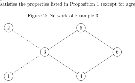
Figure 2: Network of Example 3
1 2
3
4 5
6
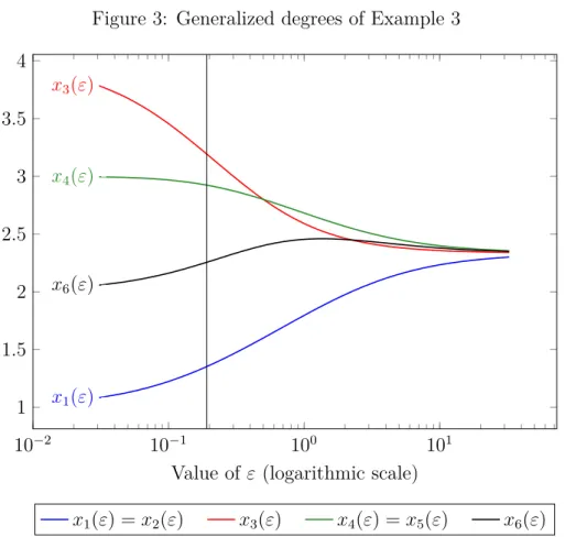
Example 3. Consider the network on Figure 2 where both normal and dashed lines indicate connections. Generalized degrees with various values of 𝜀 are given on Figure 3.
Nodes 1 and 2, and 4 and 5 are symmetric thus the two pairs have the same centrality for any parameter values. Degree gives the ranking 3≻(4∼5)≻6≻(1∼2). Generalized degrees of nodes 3, 4 and 5 monotonically decrease, while generalized degree of nodes 1
Figure 3: Generalized degrees of Example 3
10−2 10−1 100 101
1 1.5 2 2.5 3 3.5 4
𝑥1(𝜀) 𝑥3(𝜀)
𝑥4(𝜀)
𝑥6(𝜀)
Value of 𝜀 (logarithmic scale)
𝑥1(𝜀) = 𝑥2(𝜀) 𝑥3(𝜀) 𝑥4(𝜀) = 𝑥5(𝜀) 𝑥6(𝜀)
and 2 increases. However, the centrality of node 6 is not monotonic, for certain 𝜀-s it becomes larger than its limit of 7/3 (see the property agreement in Proposition 1).
It results in two changes in the centrality ranking with the watersheds of𝜀1 = 1/2 and 𝜀2 =(︁2 +√
6)︁/2. In the case of 0 < 𝜀 < 𝜀1 the central node is 3, while for 𝜀 > 𝜀1 the suggestion is 4 and 5. If 𝜀 > 𝜀2, then node 6 becomes more central than node 3.
3 An axiomatic review of generalized degree
The interpretation of generalized degree on the network gives few information about the appropriate value of parameter 𝜀. Here we use the axiomatic approach in order to get an insight into it. After the introduction of some simple, basic properties, it will be examined whether generalized degree satisfies them.
Freeman (1979) remarks that all centrality measures have an implicit starting point:
the central node of a star is the most central possible position.
Definition 5. Star center base (𝑆𝐶𝐵): Let (𝑁, 𝐴)∈ 𝒩𝑛 be a star network with 𝑖 ∈𝑁 at the center, that is, 𝑎𝑖𝑗 = 1 for all 𝑗 ̸=𝑖 and 𝑎𝑗𝑘 = 0 for all 𝑗, 𝑘 ∈𝑁 ∖ {𝑖}. Centrality measure 𝑓 :𝒩𝑛 →R𝑛 is star center based if 𝑓𝑖(𝑁, 𝐴)> 𝑓𝑗(𝑁, 𝐴) for all 𝑗 ∈𝑁 ∖ {𝑖}.
Sabidussi (1966, Definition 1) introduces five properties for a centrality measure, approved by Nieminen (1974), too. It is easy to verify that 𝒩 is closed under isomorphism (A1) as well as under the transformations switching an edge and adding an edge (A2).
Anonymity corresponds to the third axiom (A3). The other two, (A4) and (A5), deal with the consequences of switching an edge and adding an edge. They will be defined with respect to the centrality ranking.
Definition 6. Switching rank monotonicity (𝑆𝑅𝑀): Let (𝑁, 𝐴)∈ 𝒩𝑛 be a network and 𝑖, 𝑗, 𝑘 ∈𝑁 be three distinct nodes such that 𝑎𝑖𝑗 = 0 and 𝑎𝑗𝑘 = 1. Let (𝑁, 𝐴′)∈ 𝒩𝑛 be a network such that 𝐴′ =𝐴 but 𝑎′𝑖𝑗 = 1 and 𝑎′𝑗𝑘 = 0. Centrality measure 𝑓 :𝒩𝑛 →R𝑛 is switching rank monotonic if 𝑓𝑖(𝑁, 𝐴)≥𝑓ℓ(𝑁, 𝐴)⇒𝑓𝑖(𝑁, 𝐴′)≥𝑓ℓ(𝑁, 𝐴′) and 𝑓𝑖(𝑁, 𝐴)>
𝑓ℓ(𝑁, 𝐴)⇒𝑓𝑖(𝑁, 𝐴′)> 𝑓ℓ(𝑁, 𝐴′) for all ℓ∈𝑁 ∖ {𝑖, 𝑗, 𝑘}.3
Definition 7. Adding rank monotonicity: (𝐴𝑅𝑀) Let (𝑁, 𝐴) ∈ 𝒩𝑛 be a network and 𝑖, 𝑗 ∈ 𝑁 be two distinct nodes such that 𝑎𝑖𝑗 = 0. Let (𝑁, 𝐴′) ∈ 𝒩𝑛 be a network such that 𝐴′ = 𝐴 but 𝑎′𝑖𝑗 = 1. Centrality measure 𝑓 : 𝒩𝑛 → R𝑛 is adding rank monotonic if 𝑓𝑖(𝑁, 𝐴) = 𝑓𝑘(𝑁, 𝐴) ⇒𝑓𝑖(𝑁, 𝐴′) ≥ 𝑓𝑘(𝑁, 𝐴′) and 𝑓𝑖(𝑁, 𝐴) > 𝑓𝑘(𝑁, 𝐴)⇒ 𝑓𝑖(𝑁, 𝐴′) >
𝑓𝑘(𝑁, 𝐴′) for all 𝑘∈𝑁 ∖ {𝑖, 𝑗}.
Following Sabidussi (1966) and Nieminen (1974), the transformations of the original network (𝑁, 𝐴) in Definitions 5 and 6 are called switching an edge to 𝑖 andadding an edge to 𝑖, respectively.
We think they capture the essence of dynamic monotonicity. 𝑆𝑅𝑀 means that switching an edge to 𝑖is always favorable for 𝑖. 𝐴𝑅𝑀 implies that, from adding an edge between 𝑖 and𝑗, other nodes cannot benefit more than the nodes involved with respect to the centrality ranking of nodes. The supplementary conditions exclude the possibility that 𝑖 is more central than another node in the network (𝑁, 𝐴) but they are tied in (𝑁, 𝐴′).
According to our knowledge, 𝐴𝑅𝑀 was first introduced by Chien et al. (2004) for directed graphs. Boldi and Vigna (2014) also argue for the use of rank monotonicity in order to exclude pathological, counter-intuitive changes in centrality. However, they leave the study of such an axiom for future work. A review of other monotonicity axioms can be found in Landherr et al. (2010) and Boldi and Vigna (2014).
Sabidussi (1966)’s condition (A4) requires that 𝑓𝑖(𝑁, 𝐴′) > 𝑓𝑖(𝑁, 𝐴), 𝑓𝑗(𝑁, 𝐴′) >
𝑓𝑗(𝑁, 𝐴) and 𝑓𝑘(𝑁, 𝐴′) ≥ 𝑓𝑘(𝑁, 𝐴) for all 𝑘 ∈ 𝑁 ∖ {𝑖, 𝑗} after adding an edge between nodes 𝑖 and 𝑗. It seems to be not enough for us since it does not exclude the case 𝑓𝑖(𝑁, 𝐴) > 𝑓𝑘(𝑁, 𝐴) and 𝑓𝑖(𝑁, 𝐴′) < 𝑓𝑘(𝑁, 𝐴′) for some 𝑘 ∈ 𝑁 ∖ {𝑖, 𝑗}. Sabidussi (1966)’s other condition (A5) demands 𝑓𝑖(𝑁, 𝐴′)> 𝑓𝑖(𝑁, 𝐴) and 𝑓𝑖(𝑁, 𝐴)≥𝑓𝑘(𝑁, 𝐴)⇒ 𝑓𝑖(𝑁, 𝐴′) ≥ 𝑓𝑘(𝑁, 𝐴′) for all 𝑘 ∈ 𝑁 ∖ {𝑖, 𝑗} if 𝑓𝑖(𝑁, 𝐴) ≥ 𝑓ℓ(𝑁, 𝐴) for all ℓ ∈ 𝑁 after switching or adding an edge to node 𝑖. It is close to our requirements 𝑆𝑅𝑀 and 𝐴𝑅𝑀, but restricts the axiom to the elements of the center (nodes with the highest centrality).
Note that the centrality measure associating a constant value to every node of every network satisfies 𝑆𝑅𝑀 and 𝐴𝑅𝑀 but does not meet 𝑆𝐶𝐵. Degree is star center based, switching and adding rank monotonic.
Proposition 2. Generalized degree satisfies 𝑆𝐶𝐵.
Proof. Let 𝑥ℓ = 𝑥ℓ(𝜀)(𝑁, 𝐴) for all ℓ∈𝑁. Due to anonymity (see Proposition 1), 𝑥𝑗 =𝑥𝑘 for any 𝑗, 𝑘 ∈𝑁 ∖ {𝑖}. Definition 4 gives two conditions for the two variables:
[1 +𝜀(𝑛−1)]𝑥𝑖−𝜀(𝑛−1)𝑥𝑗 = 𝑛−1 (1 +𝜀)𝑥𝑖−𝜀𝑥𝑗 = 1.
It can be checked that the solution is 𝑥𝑖 = (𝑛−1)(1 + 2𝜀)
1 +𝜀𝑛 and 𝑥𝑗 = 1 +𝜀(2𝑛−1) + 2𝜀2(𝑛−1) (1 +𝜀)(1 +𝜀𝑛) ,
3Note that implication (⇒) is the same as equivalence (⇔) by changing the role of (𝑁, 𝐴) and (𝑁, 𝐴′).
hence
𝑥𝑖−𝑥𝑗 = 𝑛−2 +𝜀(𝑛−2) (1 +𝜀)(1 +𝜀𝑛) >0.
o 𝑆𝐶𝐵 means only a validity test, it is a natural requirement for any centrality measure.
Proposition 3. Generalized degree satisfies 𝑆𝑅𝑀.
Proof. Let 𝑥ℓ = 𝑥ℓ(𝜀)(𝑁, 𝐴) and 𝑥′ℓ = 𝑥ℓ(𝜀)(𝑁, 𝐴′) for all ℓ ∈ 𝑁. Let 𝑢 = 𝑥′𝑖−𝑥𝑖 and 𝑣 = max{𝑥′ℓ−𝑥ℓ :𝑗 ∈𝑁 ∖ {𝑖}}=𝑥′𝑚−𝑥𝑚. It will be verified that 𝑢≥𝑣.
Assume to the contrary that 𝑢 < 𝑣. Take the difference of equations for node 𝑚:
(𝑥′𝑚−𝑥𝑚) +𝜀 ∑︁
ℓ∈𝑁∖{𝑖,𝑚}
𝑎𝑚ℓ[(𝑥′𝑚−𝑥𝑚)−(𝑥′ℓ−𝑥ℓ)] +
+𝜀𝑎𝑚𝑖[(𝑥′𝑚−𝑥𝑚)−(𝑥′𝑖−𝑥𝑖)] = 𝑑′𝑚−𝑑𝑚 ≤0.
Since𝑣 ≥𝑥′ℓ−𝑥ℓ for allℓ∈𝑁∖{𝑖, 𝑚}, we get𝑣+𝜀𝑎𝑚𝑖(𝑣−𝑢)≤0, thus𝑣 ≤0. But switching an edge does not change the sum of degrees, therefore 0 =∑︀ℓ∈𝑁(𝑥′ℓ−𝑥ℓ)≤(𝑛−1)𝑣+𝑢,
resulting in a contradiction as 𝑢 < 𝑣 ≤0. o
Now a sufficient condition is given for generalized degree to be adding rank monotonic.
Let d= max{𝑑𝑖 :𝑖∈𝑁}be the maximal and d= min{𝑑𝑘 :𝑘∈𝑁} be the minimal degree, respectively, in a network (𝑁, 𝐴)∈ 𝒩.
Theorem 1. If
(d−d)[︁(2d+ 4)𝜀3+ 2𝜀2+𝜀]︁≤1, then generalized degree satisfies 𝐴𝑅𝑀.
The proof of this statement is not elegant, therefore one can see it in the Appendix.
In a certain sense, the result of Theorem 1 is not surprising because degree satisfies 𝐴𝑅𝑀 andx(𝜀) is close to it when 𝜀 is small.4 Our main contribution is the calculation of a sufficient condition. Note that it depends only on the minimal and maximal degree as well as on 𝜀 but not on the the number of nodes. It is always satisfied for a regular network where d=d. The value of 𝜀 is decreasing in the maximal degree and, especially, in the difference of maximal and minimal degree. However, it does not become extremely small for sparse networks with a relatively few edges compared to the number of nodes.
Parameter𝜀 is called reasonable if it satisfies (d−d) [(2d+ 4)𝜀3+ 2𝜀2+𝜀]≤1 for the network (𝑁, 𝐴)∈ 𝒩.
Remark 2. Generalized degree satisfies 𝐴𝑅𝑀 for any reasonable 𝜀 >0.
Note the analogy to the (dynamic) monotonicity of generalized row sum method (Chebotarev, 1994, Property 13).
It can be checked that generalized degree satisfies Sabidussi (1966)’s original axioms, too, if𝜀 is reasonable. Sabidussi (1966) gives only degree as a centrality measure satisfying the five conditions.
Similarly to Sabidussi (1966), strict inequalities can be demanded in𝑆𝑅𝑀 and 𝐴𝑅𝑀 (i.e. switching or adding an edge to 𝑖eliminates ties with 𝑖in the centrality ranking) but it does not affect our discussion, all results remain valid with a corresponding modification of inequalities.
According to the following example, violation of 𝐴𝑅𝑀 can be a problem in practice.
4 There exists an appropriately small𝜀satisfying the condition of Theorem 1 for anydandd.
Example 4. Consider the networks (𝑁, 𝐴),(𝑁, 𝐴′) ∈ 𝒩6 on Figure 2, where (𝑁, 𝐴) is given by the normal edges and (𝑁, 𝐴′) is obtained from (𝑁, 𝐴) by adding the two dashed edges between nodes 1 and 3, and nodes 2 and 3.
Axiom𝐴𝑅𝑀 demands that 𝑥𝑖(𝜀)(𝑁, 𝐴)≥𝑥𝑘(𝜀)(𝑁, 𝐴)⇒𝑥𝑖(𝜀)(𝑁, 𝐴′)≥𝑥𝑘(𝜀)(𝑁, 𝐴′) and 𝑥𝑖(𝜀)(𝑁, 𝐴) > 𝑥𝑘(𝜀)(𝑁, 𝐴) ⇒ 𝑥𝑖(𝜀)(𝑁, 𝐴′) > 𝑥𝑘(𝜀)(𝑁, 𝐴′) for all 𝑖 = 1,2,3 and 𝑗 = 4,5,6. However, 𝑥3(𝜀 = 3)(𝑁, 𝐴) = 𝑥6(𝜀 = 3)(𝑁, 𝐴) since nodes 3 and 6 are symmetric in (𝑁, 𝐴) but 𝑥3(𝜀= 3)(𝑁, 𝐴′)< 𝑥6(𝜀= 3)(𝑁, 𝐴′) as can seen on Figure 3. It is difficult to argue for this ranking since nodes 1 and 2 are only connected to node 3.5
The root of the problem is the excessive influence of neighbors’ degrees: the low values of 𝑑1 and 𝑑2 decrease generalized degree of node 1 despite its degree becomes greater. For large 𝜀-s this effect is responsible for breaking of the property 𝐴𝑅𝑀.
Theorem 1 gives the condition of reasonableness as 30𝜀3+ 6𝜀2+ 3𝜀≤1,
because d=𝑑3 =𝑑4 =𝑑5 = 3 andd=𝑑1 =𝑑2 = 0. It is satisfied if 𝜀 ≤ 1
15
⎛
⎝
3
√︃
266 + 15√ 334
4 − 13
√︁3
532 + 30√ 334
−1
⎞
⎠≈0.1909.
This upper bound of 𝜀 is indicated by the vertical line on Figure 3. Note that 𝐴𝑅𝑀 is violated only if 𝜀 >(︁2 +√
6)︁/2 according to Example 3, Theorem 1 does not give a necessary condition for 𝐴𝑅𝑀.
It is worth to scrutinize the connection of degree and generalized degree further.
Example 3 verifies that generalized degree (with an appropriate value of 𝜀) is not only a tie-breaking rule of degree, there exists networks where a node with a smaller degree has a larger centrality by x(𝜀).
A special type of networks is provided by a given degree sequence. Then degree of nodes is fixed along with the reasonableness of 𝜀 (depending only on degrees), while generalized degree may result in different rankings.
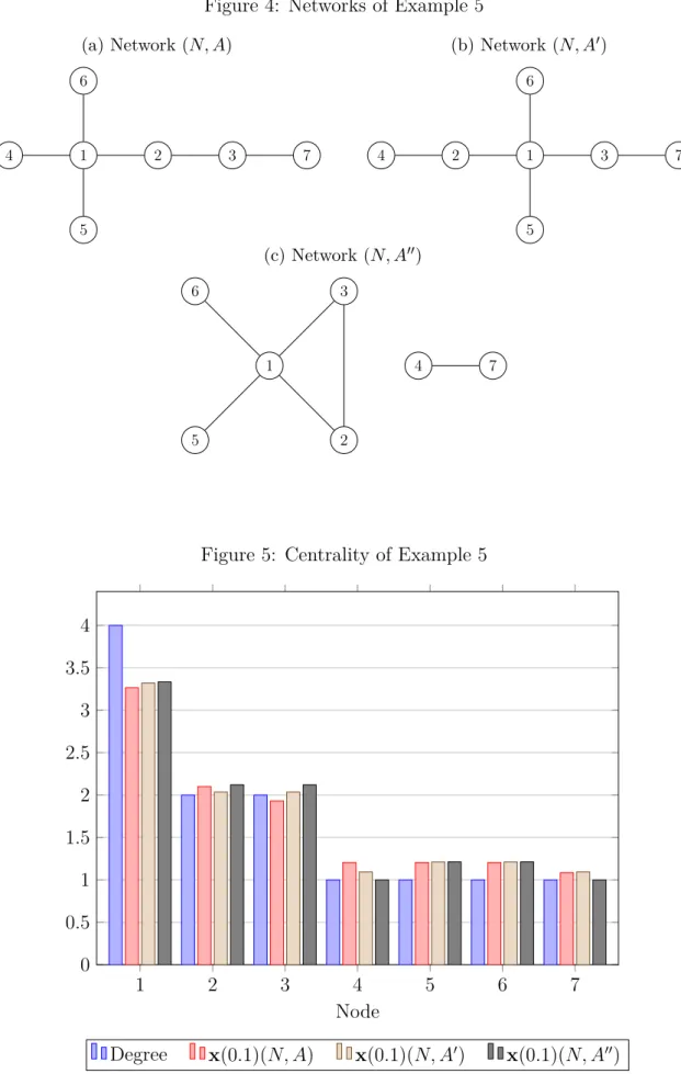
Example 5. Consider the degree sequence d = [4, 2, 2, 1, 1, 1, 1]⊤. There exist three networks with this attribute up to isomorphism, depicted on Figure 4.6 It can be checked that 𝜀= 0.1 is reasonable. Generalized degrees with this value are presented on Figure 5.
Degree provides the centrality ranking 1≻(2∼3)≻(4∼5∼6∼7) in all networks.
For (𝑁, 𝐴) (Figure 4.a), generalized degree results in 1 ≻ 2 ≻ 3 ≻ (4 ∼ 5 ∼ 6) ≻ 7 as nodes 4, 5 and 6 are symmetric, they are closer to the center 1 than 7, which is also the case with nodes 2 and 3.
For (𝑁, 𝐴′) (Figure 4.b), generalized degree gives the ranking 1 ≻(2 ∼3) ≻(5 ∼6) ≻ (4∼7) as nodes 2 and 3, 4 and 7, and 5 and 6 are symmetric, and the last pair is closer
to the center than the middle pair.
For (𝑁, 𝐴′′) (Figure 4.c), generalized degree results in the ranking 1 ≻ (2 ∼ 3) ≻ (5 ∼
5 Nevertheless, the lower rank of node 3 can be explained. Landherr et al. (2010) mention cannibal- ization and saturation effects, which sometimes arise when an actor can devote less time to maintaining existing relationships as a result of adding new contacts. Similarly, the edges can represent not only opportunities, but liabilities, too. For example, a service provider may have legal constraints to serve unprofitable customers. Investigation of these models is leaved for future research.
6 See the proof athttp://www.math.unm.edu/~loring/links/graph_s09/degreeSeq.pdf.
Figure 4: Networks of Example 5 (a) Network (𝑁, 𝐴)
1 2 3
4
5 6
7
(b) Network (𝑁, 𝐴′)
1
2 3
4
5 6
7
(c) Network (𝑁, 𝐴′′)
1
2 3
4
5 6
7
Figure 5: Centrality of Example 5
1 2 3 4 5 6 7
0 0.5 1 1.5 2 2.5 3 3.5 4
Node
Degree x(0.1)(𝑁, 𝐴) x(0.1)(𝑁, 𝐴′) x(0.1)(𝑁, 𝐴′′)
6)≻(4∼7) as nodes 2 and 3, 4 and 7, and 5 and 6 are symmetric, and the last pair is connected to the center contrary to the middle pair.
Note that generalized degree is only a tie-breaking rule of degree but all changes can be justified. The centrality values may also have a meaning: 𝑥1(0.1)(𝑁, 𝐴′)> 𝑥1(0.1)(𝑁, 𝐴) as node 1 can more easily communicate with node 7 in the network (𝑁, 𝐴′), for example. It is also remarkable that𝑥2(0.1)(𝑁, 𝐴)> 𝑥2(0.1)(𝑁, 𝐴′) and𝑥5(0.1)(𝑁, 𝐴)< 𝑥5(0.1)(𝑁, 𝐴′)<
𝑥5(0.1)(𝑁, 𝐴′′) (nodes 5 and 6 are symmetric in all cases).
4 An interpretation of the measure
In the following we present the meaning of the proposed measure on the network. Let 𝐶 ∈ R𝑛×𝑛 be a matrix such that 𝑐𝑖𝑗 = 𝑎𝑖𝑗 for all 𝑖 ̸= 𝑗 and 𝑐𝑖𝑖 = d−𝑑𝑖 for all 𝑖 = 1,2, . . . , 𝑛. 𝐶 is a modified adjacency matrix with equal row sums: its diagonal elements are nonnegative but at least one of them is zero. In other words, 𝐶 = d𝐼 − 𝐿 and x(𝜀) = [𝐼+𝜀(d𝐼−𝐶)]−1d. Let introduce the notation
𝛽 = 𝜀 1 +𝜀d. It gives
x(𝜀) = 1
1 +𝜀d(𝐼−𝛽𝐶)−1d= (1−𝛽d) (𝐼 −𝛽𝐶)−1d.
Matrix (𝐼−𝛽𝐶)−1 can be written as a limit of an infinite sequence according to its Neumann series (Neumann, 1877) if all eigenvalues of 𝛽𝐶 are in the interior of the unit circle (Meyer, 2000, p. 618).
Proposition 4. Let (𝑁, 𝐴)∈ 𝒩𝑛 be a network. Then x(𝜀) = (1−𝛽d)
∞
∑︁
𝑘=0
(𝛽𝐶)𝑘d= (1−𝛽d)(︁d+𝛽𝐶d+𝛽2𝐶2d+𝛽3𝐶3d+. . .)︁. Proof. According to the Gerˇsgorin theorem (Gerˇsgorin, 1931), all eigenvalues of 𝐿 lie within the closed interval [0,2d], so eigenvalues of 𝛽𝐶 are within the unit circle if𝛽 <1/d.
It is guaranteed due to 𝛽 =𝜀/(1 +𝜀d). o
Multiplier (1−𝛽d) >0 in the decomposition of x(𝜀) is irrelevant for the centrality ranking, it just provides that ∑︀𝑛𝑖=1𝑥𝑖(𝜀) =∑︀𝑛𝑖=1𝑑𝑖.
Lemma 2. Generalized degree centrality measure x(𝜀) = lim𝑘→∞x(𝜀)(𝑘) where x(𝜀)(0) = (1−𝛽d)d,
x(𝜀)(𝑘)=x(𝜀)(𝑘−1)+ (1−𝛽d) (𝛽𝐶)𝑘d, 𝑘 = 1,2, . . . .7
Proof. It is the immediate consequence of Proposition 4. o Lemma 2 has an interpretation on the network. In the following description the multiplier (1−𝛽d) is disregarded for the sake of simplicity. Let 𝐺′ be a graph identical to the network except that d−𝑑𝑖 loops are assigned for node 𝑖. In this way balancedness is achieved with the minimal number of loops, at least one node (with the maximal degree)
7 Superscript (𝑘) indicates the centrality vector obtained after the 𝑘th iteration step.
has no loops. Graph 𝐺′ is said to be thebalanced network of 𝐺. It is the same procedure as balancing a multigraph by loops in Chebotarev (2012, p. 1495) and in Csat´o (2015), where𝐺′ is called the balanced-graph and balanced comparison multigraph of the original graph, respectively.
Initially all nodes are endowed with an own estimation of centrality by their degree.
In the first step, degree of nodes connected to the given one is taken into account: 𝐶d corresponds to the sum of degree of neighbors (including the nodes available on loops).
Adding d−𝑑𝑖 loops provides that the number of 1-long paths from node𝑖 is exactly d.8 Then this aggregated degree of objects connected to the given one is added to the original estimation with a weight 𝛽, resulting in d+𝛽𝐶d.
In the𝑘th step, the summarized degree of nodes available on all𝑘-long paths (including loops) 𝐶𝑘d is added to the previous centrality, weighted by 𝛽𝑘 according to the length of the paths. This iteration converges to the generalized degree ranking due to Lemma 2.
Example 6 illustrates the decomposition.
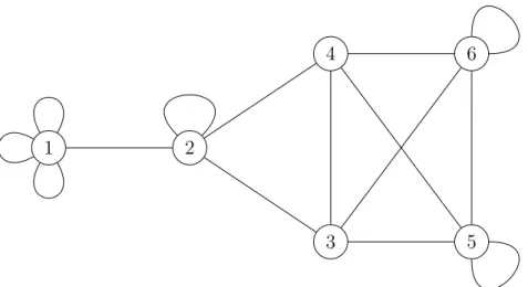
Figure 6: Network of Example 6
1 2
3 4
5 6
Example 6. Consider the network whose balanced network is shown on Figure 6, where the number of loops are determined by the differences d−𝑑𝑖. Nodes 3 and 4, and 5 and 6 are symmetric, the two pairs have the same centrality for any 𝜀. Generalized degree gives the rather natural ranking of (3∼4)≻(5∼6)≻2≻1.
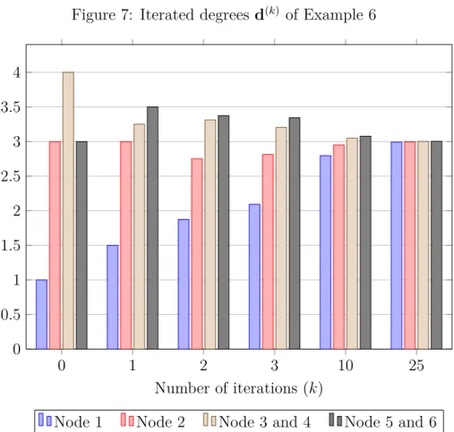
Figure 7 shows the average degree of neighbors available along a𝑘-long path for various 𝑘-s, that is, d(𝑘) = [(1/d)𝐶]𝑘d. Their sum is equal to ∑︀𝑛𝑖=1𝑑𝑖. Lemma 2 means that, for instance, x(𝜀)(2) = (1−𝛽d)[︁d(0)+𝛽dd(1)+𝛽2d2d(2)]︁. It reveals that nodes 5 and 6 are connected to more central nodes than 3 and 4. Another interesting fact is that d(𝑘) is monotonic only in its first coordinate. The elements of d(25) are almost equal, large powers does not count much. Now x(𝜀)(1) immediately gives the final ranking of nodes.
Two observations can be taken on the basis of examples scrutinized. The first is that ties in degree are usually eliminated after taking the network structure into account, which
8 In the limit it corresponds to the average degree of neighbors in𝐺′ since lim𝜀→∞𝛽= 1/d.
Figure 7: Iterated degrees d(𝑘) of Example 6
0 1 2 3 10 25
0 0.5 1 1.5 2 2.5 3 3.5 4
Number of iterations (𝑘)
Node 1 Node 2 Node 3 and 4 Node 5 and 6
can be advantageous in practical applications: in the analysis of terrorist networks, a serious problem can be that standard centrality measures struggle to identify a given number of key thugs because of ties (Lindelauf et al., 2013). In other words, generalized degree has a good level of differentiation.
The second is the possibly slow convergence: in a sparse graph, long paths should be considered in order to get the final centrality ranking of the nodes, however, it is not clear why they still have some importance. Since the iteration depends on the network structure, it will be challenging to give an estimate for how many iteration steps are necessary to approach the final centrality.
5 Conclusion
The paper has introduced a new centrality measure called generalized degree. It is based on degree and the Laplacian matrix of the network graph. The method carries out a redistribution of the pool filled with the sum of degrees. The effect of neighbors centrality is controlled by a parameter, placing our method between degree and equal centrality for all nodes of a component. Inspired by the idea of Sabidussi (1966), two rank monotonic axioms have been defined, and a sufficient condition has been provided in order to satisfy them. Besides PageRank (Chien et al., 2004), we do not know any other centrality measure with these properties. Furthermore, an iterative formula has been given for the calculation of generalized degree along with an interpretation on the network.
The main advantage of our measure is its degree-based concept. It is recommended to use with a low value of 𝜀 instead of degree, which preserves most favorable properties of degree but has a much stronger ability to differentiate among the nodes and better reflect
their role in the network (see Example 6). It is especially suitable to be a tie-breaking rule of degree, possible applications involve all fields where degree is used in order to measure centrality.
Besides that, it is suggested to test various parameters and follow all changes in the centrality ranking. It is not necessary to restrict the interval to reasonable values, generalized degree may give an insight about the importance of nodes even if adding rank monotonicity is not guaranteed and its other properties remain valid.
This research has opened some ways for future work. Generalized degree can be compared with other centrality measures, for example, through the investigation of their behavior on randomly generated networks. Rank monotonicity is worth to consider in an axiomatic comparison of centrality measures in the traces of Landherr et al. (2010) and Boldi and Vigna (2014). The iterative formula and the graph interpretation may also inspire a characterization of generalized degree.
Finally, some papers have used centrality measures just to describe the network by a single value of centrality index. For instance, Sabidussi (1966) has suggested that 1/max{𝑓𝑖(𝑁, 𝐴) :𝑖 ∈ 𝑁} is a good centrality index if centrality measure 𝑓 : 𝒩𝑛 →R𝑛 satisfies the five axioms (A1)-(A5). It has been shown that generalized degree (for certain values of 𝜀) meets these requirements. Moreover, it improves on a failure of degree:
1/max{𝑑𝑖 :𝑖∈𝑁} is the same in a complete and a star network of the same order but 1/max{𝑥𝑖(𝜀) : 𝑖 ∈ 𝑁} is larger in a complete one. We think this observation deserves more attention.
Appendix
Proof of Theorem 1. Let𝑥ℓ =𝑥ℓ(𝜀)(𝑁, 𝐴) and 𝑥′ℓ =𝑥ℓ(𝜀)(𝑁, 𝐴′) for all ℓ∈𝑁. It can be assumed without loss of generality that 𝑥′𝑖−𝑥𝑖 ≥𝑥′𝑗 −𝑥𝑗. Let 𝑠= 𝑥′𝑖−𝑥𝑖, 𝑡 = 𝑥′𝑗−𝑥𝑗, 𝑢= max{𝑥′ℓ−𝑥ℓ :ℓ∈𝑁∖ {𝑖, 𝑗}}=𝑥′𝑘−𝑥𝑘and𝑣 = min{𝑥′ℓ−𝑥ℓ :ℓ∈𝑁∖ {𝑖, 𝑗}= 𝑥′𝑚−𝑥𝑚. It will be verified that 𝑡≥𝑢.
Assume to the contrary that𝑡 < 𝑢. Take the difference of equations concerning node 𝑘:
(𝑥′𝑘−𝑥𝑘) +𝜀 ∑︁
ℓ∈𝑁∖{𝑖,𝑗,𝑘}
𝑎𝑘ℓ[(𝑥′𝑘−𝑥𝑘)−(𝑥′ℓ−𝑥ℓ)] +
+𝜀𝑎𝑘𝑖[(𝑥′𝑘−𝑥𝑘)−(𝑥′𝑖−𝑥𝑖)] +𝜀𝑎𝑘𝑗[︁(𝑥′𝑘−𝑥𝑘)−(︁𝑥′𝑗 −𝑥𝑗)︁]︁ = 𝑑′𝑘−𝑑𝑘= 0.
Since 𝑢=𝑥′𝑘−𝑥𝑘 ≥𝑥′ℓ−𝑥ℓ for all ℓ∈𝑁 ∖ {𝑖, 𝑗} and 𝑢≥𝑡, we get 𝑢≤𝜀𝑎𝑘𝑖(𝑠−𝑢) ⇔ 𝑢≤ 𝜀𝑎𝑘𝑖
1 +𝜀𝑎𝑘𝑖𝑠. (1)
Now take the difference of equations concerning node𝑖:
𝑠+𝜀 ∑︁
ℓ∈𝑁∖{𝑖,𝑗}
𝑎𝑖ℓ[𝑠−(𝑥′ℓ−𝑥ℓ)] +𝜀(︁𝑥′𝑖−𝑥′𝑗)︁=𝑑′𝑖−𝑑𝑖 = 1.
Since 𝑢≥𝑥′ℓ−𝑥ℓ for all ℓ∈𝑁 ∖ {𝑖, 𝑗}, we get 𝑠+𝜀 ∑︁
ℓ∈𝑁∖{𝑖,𝑗}
𝑎𝑖ℓ(𝑠−𝑢) +𝜀(︁𝑥′𝑖−𝑥′𝑗)︁=𝑠+𝜀𝑑𝑖(𝑠−𝑢) +𝜀(︁𝑥′𝑖−𝑥′𝑗)︁≤1.
An upper bound for 𝑢is known from (1), thus 1 +𝜀(︁𝑥′𝑗−𝑥′𝑖)︁≥𝑠+𝜀𝑑𝑖(𝑠−𝑢)≥𝑠+𝜀𝑑𝑖
(︂
1− 𝜀𝑎𝑘𝑖 1 +𝜀𝑎𝑘𝑖
)︂
𝑠= 1 +𝜀𝑎𝑘𝑖+𝜀𝑑𝑖
1 +𝜀𝑎𝑘𝑖 𝑠. (2)