Research Article
Optimal Payments to Connected Depositors in Turbulent Times:
A Markov Chain Approach
Dávid Csercsik
1and Hubert János Kiss
2,31Faculty of Information Technology and Bionics, P´azm´any P´eter Catholic University, P.O. Box 278, Budapest 1444, Hungary
2MTA KRTK KTI, T´oth K´alm´an U. 4., Budapest 1097, Hungary
3Department of Economics, E¨otv¨os Lor´and University, P´azm´any P´eter S´et´any 1/a, Budapest 1117, Hungary
Correspondence should be addressed to D´avid Csercsik; csercsik@itk.ppke.hu Received 25 August 2017; Accepted 19 February 2018; Published 2 April 2018
Academic Editor: Ahmet Sensoy
Copyright © 2018 D´avid Csercsik and Hubert J´anos Kiss. This is an open access article distributed under the Creative Commons Attribution License, which permits unrestricted use, distribution, and reproduction in any medium, provided the original work is properly cited.
We propose a discrete time probabilistic model of depositor behavior which takes into account the information flow among depositors. In each time period each depositors’ current state is determined in a stochastic way, based on their previous state, the state of other connected depositors, and the strategy of the bank. The bank offers payment to impatient depositors (those who want to withdraw their funds) who accept or decline them with certain probability, depending on the offered amount. Our principal aim is to see what are the optimal offers of the bank if it wants to keep the expected chance of a bank run under a certain level and minimize its expected payments, while taking into account the connection structure of the depositors. We show that in the case of the proposed model this question results in a nonlinear optimization problem with nonlinear constraints and that the method is capable of accounting for time-varying resource limits of the bank. Optimal offers increase (a) in the degree of the depositor, (b) in the probability of being hit by a liquidity shock, and (c) in the effect of a neighboring impatient depositor.
1. Introduction
Banks and other financial intermediaries convert short-term liabilities into long-term and often illiquid assets, a process called maturity transformation. Liquidating the assets is gen- erally costly; hence if many depositors or investors attempt to withdraw their funds from the bank or from other forms of financial intermediation, then liquidity problems may arise that may spark a bank run and result in solvency problems through fire sales. If depositors anticipate such potential problems, then it may in turn make them more prone to withdraw. Moreover, during financial crisis it is even more likely that depositors are concerned about the liquidity and solvency of their bank, making bank runs more probable also.
In traditional bank run models [1, 2] banks are supposed to determine payment to those who withdraw as a result of a maximization problem. The bank maximizes the overall expected utility of its depositors. Depending on the specified environment, these models either allow a bank run outcome [1] or do not [2]. In this paper we take a different approach.
In times of crises, it makes sense to assume that the most important objective of the bank is to survive. More precisely, it wants to keep the probability of a potentially devastating bank run very low at a minimum cost. The bank’s intention to minimize the cost (in our case the payments to depositors) in times of financial distress is due to the uncertainty about the duration of the crisis and unforeseeable contingencies.
Hence, the bank wants to keep as much funds available as possible to be prepared for future potential difficulties.
However, it aims also to pay to those who withdraw smoothly so that rumours about problems of receiving a payment from the bank do not set off a bank run.
Our main aim is to understand the optimal payments of the bank during crises when the bank wants to minimize payments but also maintain sufficiently low the probability of bank runs given the connections between depositors.
Unlike in other models, depositors’ decision is assumed to be determined in the following way. Each bank customer starts as a depositor without urgent liquidity needs (i.e., they are patient in bank run parlance). However, in any period
Volume 2018, Article ID 9434608, 14 pages https://doi.org/10.1155/2018/9434608
each depositor may be hit by a liquidity shock, turning a patient depositor into an impatient one. Impatient depositors have immediate liquidity needs so they withdraw money from the bank as soon as they can. When they contact the bank to withdraw money, the bank makes them an offer that they can accept or reject. The probability of accepting the offer depends on the amount that is being offered. The larger the amount, the more likely that the depositor accepts it. Accepting or not does not only affect the bank and the depositor in question, but may have an additional effect.
Depositors are connected by an underlying social network and if a patient depositor is connected to an impatient depositor, then the probability to become impatient increases.
A possible explanation is that if a depositor notes that the number of those who want to withdraw from the bank increases, then she may interpret it as people trying to get out their funds due to some problem with the bank. In such a case it may be optimal to withdraw as well, because if a depositor waits too long while the rest withdraws, then she may have problems to recover her funds. Once an impatient depositor accepts the offer from the bank, she ceases to be impatient and her effect on other depositors disappears as well. We define a bank run as a situation in which there is no more patient depositor because everybody wants to withdraw or has done so already. We compute how the payments to depositors who want to withdraw should be so as to minimize these payments, but also to keep the probability of a bank run low, taking into account how depositors affect each other through the underlying social network.
Even though bank run models differ in important points (e.g., whether there is aggregate uncertainty about the liq- uidity needs), almost all models have multiple equilibria, one of which involves bank runs. This paper also admits bank runs as the bank sets payments in a way that the probability of runs is reduced but need not be zero. However, we do not have equilibria as depositors do not make strategic decisions. Depositors in our model react as an automaton to what happens around them, in a nonstrategic way. Our focus is on how banks determine payment optimally in such an environment. We show that the problem can be neatly formalized as an optimization problem. However, the general formulation is too complex to be analyzed. Hence, we focus in detail on a small, tractable problem. We find that depositors with more connections receive larger optimal offers from the bank,ceteris paribus, reflecting the idea that the bank attempts to avoid that these depositors increase the probability that the depositors they are connected to become also impatient. We also find that the lower is the probability of bank runs that a bank tolerates, the larger is the optimal offer, all other things held constant. It is intuitive because through larger offers the bank reduces the probability of rejected offers that may lead to a bank run. As expected, the optimal payment to impatient depositors increases as the probability of liquidity shocks increases. In our examples, the optimal offers are almost linear in the probability of being hit by the liquidity shock, but the expected cost increases often nonlinearly in the same parameter. We show also through our example that the larger is the effect that an impatient depositor exerts on her neighbors, the larger is the optimal
offer, ceteris paribus. We find also that the sparser is the connection structure between depositors, the less they affect each other; hence the optimal offers from the bank are also smaller. We show also that the same analysis can be carried out in more complicated models that take into account feasibility constraints and allow for time-varying offers. Most importantly, even in these more intricate setups we find that more connected depositors receive larger offers from the bank.
There are several institutions and policies that are designed to handle problems that may arise during crises.
The most prominent is deposit insurance that guarantees the recovery of deposits in case the bank has liquidity or other problems. There are several issues that make deposit insurance an imperfect solution. It entails moral hazard since the insurance of deposits may motivate banks to take on excessive risks. The coverage is limited both in size and scope, so depositors with a large deposit and investors with uninsured investments still remain a concern for the bank.
For these reasons other ways of coping with financial distress have been used also. The most frequent alternative is liquidity suspension and rescheduling of payments. Our paper can be viewed as an attempt to formalize how this rescheduling should be if connections between depositors matter and the bank aims at minimizing payments to depositors but also wants to keep the probability of bank runs low. In many instances, the renegotiation of payments is done by the banking authority. Ennis and Keister [3] have examples of how such rescheduling occurred in some countries.
Note that many nonbank institutions (like mutual funds) engage also in maturity transformation and in their case short-term liabilities also retain a debt-like structure. Gener- ally, the investments these institutions have are susceptible to investor run as well. In general, consider any firm or financial institution that owes to investors and negotiates with them about the terms of repayment, knowing that those investors may be connected. Our analysis applies to them as well. A further motivating example may be countries that struggle to pay their sovereign debt. Consider for instance Argentina that restructured its debt several times in the last decade. During this process the affected bondholders are offered payments (often in form of longer term bonds) that are lower than the original bonds promised. Obviously, the country that is dealing with the bondholders tries to minimize the payments but wants the bondholders to accept the offers it makes.
If a bondholder accepts an offer, then it may influence the willingness of other bondholders to accept the offer as well [4].
Next we show that that depositors react to the decisions of other depositors that they observe and then discuss issues related to the importance of setting the right payment to depositors.
In our model, depositors react to other depositors’
observed decisions. More precisely, we assume that the chance that a depositor becomes impatient is growing in the number of impatient depositors that she is linked to.
Empirical studies support this idea. Kelly and O’Grada [5]
investigate a bank run episode in New York in the 19th century and show that the most important factor determining
whether an individual panicked or not was her county of origin in Ireland. Immigrants from the same country clustered in the same neighborhood and observed each other, so if a depositor saw a large number of individuals trying to withdraw, then she was more likely to do so as well. Iyer and Puri [6] study a bank run that occurred in India in 2001 and demonstrate that observing withdrawals in one’s social network increases the probability that the depositor in question follows suit. Starr and Yilmaz [7] show that, during a bank run incident in 2001 that occurred in Turkey, small and medium-sized depositors of an Islamic bank seemed to observe withdrawals of their peers and the larger the mass that withdrew, the more depositors did the same the next day.
Experimental evidence also suggests that observability plays an important role in the emergence of bank runs (see, e.g., [8–
11]). A common finding of these experimental studies is that if previous withdrawals are observed, then they induce fur- ther withdrawals. These empirical and experimental findings make it clear that depositors are affected by the withdrawal decision of depositors they are connected to. That is why we consider it important to introduce this feature into our model.
In the theoretical literature banks are supposed to act in the interest of the depositors and hence they set payments in a way that maximizes the overall utility of depositors.
Important for our study, Green and Lin [2] find that the optimal payment depends on the self-reported type of the depositors and their position in the sequence of decision. As a consequence, depositors who withdraw early may end up with quite different payments. Our model has that feature as well, although in our case differences in payments are due to the connection structure between depositors. Ennis and Keister [3] use a Diamond and Dybvig [1] model and show that if the bank realizes that a bank run is underway, then it reoptimizes the payments to the subsequent depositors.
Our idea is similar in the sense that the bank adapts to hard times, but the optimization problem in our model is very different. Unlike [3], we do not maximize the utility of the remaining depositors but minimize the payments to them so that they accept it with sufficiently large probability and do not ignite a bank run. Considering that reactions to the first withdrawal may appear within days (or even hours), this seems to be a plausible scenario. According to this, the most straightforward interpretation for the discrete time periods of our model is the scale of days.
Note that as the depositors in our model are automatons that do not decide in a strategic way to maximize their own utilities and neither does the bank set payments in order to maximize the overall utility of the depositors, this study is clearly not a strictly neoclassical economic model for bank runs.
We are aware of only one paper that uses Markov chains to study bank runs. Temzelides [12] studies how depositors are affected by the number of withdrawals from their and other banks in the previous period. He investigates myopic best response in an evolutionary banking setup. In his model there is no underlying social network that determines who affects whom, but each depositor observes other depositors’
past action. Neither does he study the optimal payment, so our approaches are quite different.
2. Materials and Methods
Assume that there are𝑛depositors that are located at the nodes of a network and connections enable observability.
Hence, a link connecting two depositors implies that they can observe each other’s action.
To define a Markov chain model, we have to specify the possible states of the model and the state transition matrix 𝑄which contains the state transition probabilities. Since the connections of a certain depositor to another ones matter, we will distinguish them. This means that the set of the possible states of the model (S) can be determined as the Descartes product over the set of possible states of the depositors (𝑆).
To keep the model as simple as possible, we will assume three possible state for each depositor:
(i)Patient(𝑃): this is the basic state of each depositor and following the literature a patient depositor does not have urgent liquidity need.
(ii)Impatient (𝐼): if a liquidity shock hits a depositor, her state changes from𝑃 to𝐼, meaning that she is demanding money from the bank. Furthermore, if two depositors are connected and one is impatient, she increases the probability of the other one becom- ing impatient. We assume that this effect is additive, so two impatient acquaintances double the chance of a𝑃 → 𝐼transition.
(iii)Out (𝑂): we assume that the bank offers a certain amount of money to impatient depositors, who may accept or reject the offer. We suppose that the chance that the impatient depositor accepts the offered quan- tity increases with the offered sum. If the depositor accepts the offered amount of money, her state will turn from𝐼to𝑂and ceases to affect her neighbors thereafter. If she rejects, then she stays in state𝐼for the next step.
Hence, 𝑆 = {𝑃, 𝐼, 𝑂}. Note that all depositors start being patient and then may turn impatient. Those impatient depositors who accept the offer of the bank enter state𝑂. It is not possible to go directly from𝑃to𝑂and any move in the reverse direction (for example from𝐼to𝑃) is disregarded also. Given this setup, the total number of states of the system will be3𝑛where𝑛is the number of depositors. For the sake of tractability we use the following assumptions:
(i)Connection structure: the structure of the links con- necting the depositors may be described by a simple undirected graph, whose adjacency matrix is 𝐴(a straightforward generalization of the model could be where we assume asymmetric information, and thus a directed A). Take any two depositors. If they are linked, then the corresponding entry in the adjacency matrix is 1. If one of them is impatient, while the other one is patient, then the former affects the latter one by increasing the probability that it turns impatient as well. Following the standard language of network analysis, if two depositors are connected, then they are neighbors, and the number of connections a depositor has is called degree. Hereafter, we assume that the
bank knows the connection structure. We admit that this is a strong assumption, but banks may have a lot of information about depositors including information about connections between them. Based on [5, 6], depositors living in the same neighborhood are likely to observe each other. Starr and Yilmaz [7] suggest that deposit size also may be a determinant of which depositor observes which other depositors. Banks may take into account such information.
(ii)Homogeneity: depositors are homogeneous in the following senses: (i) the chance of being hit by the liquidity shock is the same for all patient depositors (and independent of the degree); (ii) when offered a certain amount by the bank, the probability of accepting that amount (and hence change into the state𝑂) is also the same for all impatient depositors (and again independent of the degree).
(iii)Degree-dependent payments: let𝑜𝑖,deg(𝑖)(𝑡)be the sum offered to depositor𝑖 at time 𝑡where deg(𝑖) is the number of neighbors of 𝑖. The bank distinguishes depositors based only on their degree. In other words, assuming time-independent payments, two deposi- tors with the same degree receive always the same offer from the bank if in any given state and time.
Since 𝑜𝑖,deg(𝑖)(𝑡) = 𝑜𝑗,deg(𝑗)(𝑡) if deg(𝑖) = deg(𝑗), hereafter we use𝑜deg(𝑖)(𝑡).
Note that the assumptions on the connection structure and homogeneity imply that depositors in the model differ only in their degree. As a consequence, there are2𝑛−1possible connection structures.
2.1. State Transition Probabilities. Now we are ready to define the state transition probabilities. Any state 𝜎 in S can be composed as 𝑠1𝑠2⋅ ⋅ ⋅ 𝑠𝑛 where 𝑠𝑖 ∈ 𝑆 = {𝑃, 𝐼, 𝑂}. Let us furthermore use the following notation convention: 𝜎(𝑡, 𝑖) denotes𝑠𝑖(𝑡), the state of depositor𝑖at time𝑡.
Within a given time period, we assume that the following events take place simultaneously:
(i) Patient depositors turn impatient with some probabil- ity (that is determined by the probability of being hit by the liquidity shock and the number of impatient neighbors).
(ii) Impatient depositors decide if they accept or reject the offers by the bank.
We assume that transition events of the depositors in one step are independent, so the transition probability from state 𝜎(1) = 𝑠1(1)𝑠2(1) ⋅ ⋅ ⋅ 𝑠𝑛(1) at 𝑡 = 1 to 𝜎(2) = 𝑠1(2)𝑠2(2) ⋅ ⋅ ⋅ 𝑠𝑛(2)at𝑡 = 2can be written as
𝑝 (𝜎 (1) → 𝜎 (2)) =∏𝑛
𝑖=1
𝑝 (𝑠𝑖(1) → 𝑠𝑖(2)) , (1) where𝑝(𝑠𝑖(1) → 𝑠𝑖(2))denotes the probability that depositor 𝑖changes her state from𝑠𝑖(1)to𝑠𝑖(2)where𝑠𝑖(1), 𝑠𝑖(2) ∈ 𝑆.
Next, we determine the single transition probabilities.
(i) The chance of a liquidity shock hitting each patient depositor at each time period is denoted by𝑝𝑠. We assume that impatient depositors affect the behavior of patient neighbors and may induce𝑃 → 𝐼transi- tions:𝛿denotes the level of how much an impatient depositor connected to a patient one increases the 𝑃 → 𝐼 transition. This way the patient-impatient transition at time 𝑡 for patient depositor𝑖 may be calculated as
𝑝𝑠+ 𝑘𝐼𝑖(𝑡) 𝛿, (2) where 𝑘𝐼𝑖(𝑡) is the number of impatient depositors connected to𝑖at time𝑡(in general we do not assume the connection structure to change, but the model framework is capable of handling such cases). The chance of staying in the𝑃state is1 − 𝑝(𝑃 → 𝐼).
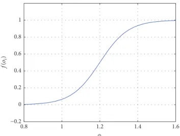
(ii) The chance that an impatient depositor𝑖accepts the offered money at time 𝑡 is denoted by 𝑓(𝑜deg(𝑖)(𝑡)) where𝑓is a monotone increasing function, assumed to be the same for each depositor. The chance of staying in the𝐼state is1 − 𝑝(𝐼 → 𝑂).
To characterize the evolution of the system we introduce a lexicographic ordering of the states (e.g.,𝑃𝑃𝑃 ⋅ ⋅ ⋅ 𝑃𝑃 = 𝜎1; 𝑃𝑃𝑃 ⋅ ⋅ ⋅ 𝑃𝐼 = 𝜎2; e.g., see Appendix A). Furthermore, we define the state transition matrix𝑄 ∈ R3𝑛×3𝑛.𝑄𝑖,𝑗 is equal to the probability of the transition from state𝜎𝑖 to𝜎𝑗. The probability of state𝑖at time𝑡is given by the𝑖th element of the vector𝑝(𝑡) ∈R3𝑛. We will denote the probability of state 𝑗 (𝜎 = 𝜎𝑗)at time𝑡shortly with𝑝𝑡𝑗(𝑝𝑡𝑗equals the𝑗th element of𝑝(𝑡)). Therefore,
𝑝 (𝑡) = (𝑄𝑇)𝑡𝑝 (0) , (3) where 𝑝(0) ∈ R3𝑛 is a vector describing the initial state of the system. Thus,𝑝(0) = (1, 0, 0, . . . , 0)denotes that the probability of the initial state (in our lexicographic ordering 𝜎1= 𝑃𝑃𝑃 ⋅ ⋅ ⋅ 𝑃) is 1.
Let us define the cost of a given state𝜎at time𝑡as the sum of offers accepted in the last time period (corresponding to𝐼 → 𝑂transitions from𝑡 − 1to𝑡)
𝑐 (𝜎 (𝑡)) = ∑
𝑗:𝜎(𝑡,𝑗)=𝑂,𝜎(𝑡−1,𝑗)=𝐼
𝑜deg(𝑗)(𝑡 − 1) . (4) That is, the sum of offers that have been accepted at time period𝑡 (but not before) by depositors with degree 𝑗 that ranges from 0 to𝑛 − 1. The total (or cumulated) cost (𝐶) of 𝜎(𝑡)may be defined as
𝐶 (𝜎 (𝑡)) =∑𝑡
𝑘=2
𝑐 (𝜎𝑖(𝑘)) . (5) As already pointed out, it is plausible to believe that in turbulent times banks attempt to minimize the payments to depositors who want to withdraw, but at the same time the bank tries to keep the probability of a bank run at a low level.
As we will show, with the proposed formalized model we are able to exactly grasp this intuition.
3. Results and Discussion
3.1. Optimization with No Offer Constraints and Time-Inde- pendent Offers. In this section we assume that the offers are time-independent, which means that a depositor with a certain number of neighbors receives the same offer in each time period if in impatient state (and so we omit the argument 𝑡in𝑜deg(𝑖)(𝑡)).
Let𝐸[𝐶(𝑡)]denote the expected payments to depositors at time𝑡. In general,
𝐸 [𝐶 (𝑡)] = ∑
𝑖
𝐶 (𝜎𝑖(𝑡)) 𝑝𝑖(𝑡) , (6) where𝑝𝑖(𝑡)is the probability of state𝜎𝑖at time𝑡, which may be calculated from𝑥(𝑡). However, since the offers are time- independent, we may write
𝐸 [𝐶 (𝑡)] = ∑
𝑗:𝑂∈𝜎𝑗
𝑜deg(𝑗)𝑝𝑖(𝑡) , (7) so we omit the argument𝑡in𝑜deg(𝑖)(𝑡).
Assuming time-independent offers, the expected cost of the bank𝐸[𝐶(𝑡)]depends on the probability of those states at time𝑡, which have at least one𝑂, and the position of those𝑂- s in𝜎. The position determines the degree which determines the payment (since payments only depend on the depositors’
degree) to those depositors that were impatient and accepted the offer.
Actual payments are made only to those impatient depos- itors who accept the offer. Since offers are assumed to be time- independent, in this case it does not matter when the given state changed from𝐼to𝑂(in other words, when the offer was accepted), since amounts offered for a certain (impatient) node are time-independent.
To formulate the optimization problem, we also need to define what we consider a bank run.
Definition 1. Any state where no patient depositor is present is considered as a bank run event. The probability of a bank run event at time𝑡is denoted by𝑃BR(𝑡)(note the irreversibility:
since there is no 𝑂 → 𝐼, 𝑂 → 𝑃, or 𝐼 → 𝑃 transition, once the system is in a state of bank run event, all following states will be bank run events).
The precise interpretation of the above event is that for a time instance𝑡 a bank run is present at time𝑡 or it has already occurred before. Intuitively, we assume that the bank run itself means that active depositors are present, who are all impatient. Since the state where all depositors are in the state𝑂also fulfills the definition, it is contra-intuitive in the sense that at that time the bank run is already over. However if all depositors are in the state𝑂, it is sure that a bank run has already occurred.
The optimization problem of the bank is the following at time𝑡and given a connection structure𝐴:
𝑜min1,...,𝑜𝑑 𝐸 [𝐶 (𝑡)]
subject to 𝑃BR(𝑡) < 𝑃BR, (8)
1
2 3
Figure 1: Topology 1: connection of the depositors in the case of Example 1.
where𝑑is the maximal degree in the connection structure, and
𝑃BR(𝑡) = ∑
𝑖:𝑃∉𝜎𝑖
𝑝𝑖(𝑡) , (9)
where 𝑃 ∉ 𝜎𝑖 refers to those states which do not include patient (𝑃) depositors.𝑃BR(𝑡) < 𝑃BRdenotes that we want to keep the probability of bank run event below some given threshold.
While this is a general optimization, it is too complex to be analyzed. The size of the state transition matrix grows exponentially with the number of the modelled depositors, and the complexity of the resulting expressions may be very high even in the case of quite simple examples that we show next. One may partially overcome this problem by merging states or doing simplifications regarding the Markov chain model. Moreover, nonlinear optimization problems with nonlinear constraints such as, for example, (8), are not easy to handle, and the solvers may run into local extrema (Bertsekas 1999). Furthermore, the needed computing capacity may be also significant due to the complexity of the functions. For these reasons, in the rest of the paper we limit ourselves to small examples to gain insight into how the optimal payments and expected costs vary as the environment changes.
In this section we assume that the quantities offered by the bank to the impatient depositors are not constrained by any consideration regarding their upper bound. In other words, the bank may offer arbitrarily high sums in order to control the expected chance of a bank run event; there is no feasibility constraint.
3.1.1. Example 1. Consider an example with three depositors.
We fix the connection structure as depicted in Figure 1.
Furthermore, we assume the most simple possible case regarding the function𝑓that determines the probability of accepting an offer, namely,𝑓(𝑜deg(𝑖)) = 𝑜deg(𝑖). This implies that we assume 𝑜𝑛 ∈ [0, 1) ∀𝑛. We use a lexicographic ordering of the states described in Appendix A.
We are interested in the bank’s optimal strategy. Con- cretely, let us determine which offers should the bank make to impatient depositors, if the initial state of the system (e.g., 𝑃𝑃𝑃) is known, and the bank wants to keep the chance of a bank run event (𝑃BR) under a certain probability level while also aiming to minimize the expected cost.
At𝑡 = 1the probability of a bank run event is independent of the offered sums and is equal to𝑃BR(1) = 𝑝3𝑠. Regarding𝑡 = 2,𝑃BR(2)is equal to𝑝8(2)+𝑝15(2)+𝑝16(2)+𝑝17(2)+𝑝18(2) +𝑝19(2)+ 𝑝20(2) +𝑝21(2), which can be calculated from (3), assuming𝑥0 = [1 0 0 ⋅ ⋅ ⋅ 0]𝑇(i.e., at the beginning
each depositor is patient). Note that in Appendix A we define all potential states that may arise with three depositors, and states 8, 15, 16, 17, 18, 19, 20, and 21 are those that do not contain any patient depositor. In Appendix A, we develop the probabilities for all the possible 27 states and it yields that at 𝑡 = 2the probability of bank run event is
𝑃BR(2) = 𝛿2𝑝3𝑠− 2𝛿2𝑝2𝑠+ 𝛿2𝑝𝑠+ 4𝛿𝑝4𝑠− 12𝛿𝑝3𝑠
+ 8𝛿𝑝𝑠2− 𝑝𝑠6+ 6𝑝5𝑠− 12𝑝𝑠4+ 8𝑝3𝑠, (10) which is also independent of the offers. This is not surprising.
If a depositor becomes impatient at𝑡 = 1, with the offer we may influence the probability that she changes to𝑂at𝑡 = 2.
However, regarding patient depositors (on whom the bank run event definition is based on), the important thing is how long their impatient neighbors remain in the𝐼state.
Consider the following example. At 𝑡 = 1 the state 𝐼𝑃𝑃 appears. With the offer at 𝑡 = 1 we may affect the probability of, for example,𝐼𝑃𝑃 and 𝑂𝑃𝑃at𝑡 = 2, but it makes no difference in terms of whether the next state will be considered as a bank run event or not. Recall the bank run event definition according to which, for example,𝐼𝑃𝑃and 𝑂𝑃𝑃are regarded as the same. Depositors 2 and 3 are affected by the𝐼state of player 1 at the transition from𝑡 = 1to𝑡 = 2, irrespective of the offer to depositor 1 at𝑡 = 1. On the other hand, at𝑡 = 3it matters whether depositor 1 remained in state 𝐼at𝑡 = 2as well or not (which in turn already depends on the offer).
As expected, the offers first appear in the probability of bank run at𝑡 = 3 (𝑃BR(3)):
𝑃BR(3) = 36𝛿𝑝2𝑠+ 7𝛿2𝑝𝑠− 120𝛿𝑝3𝑠 − 4𝛿3𝑝𝑠+ 156𝛿𝑝4𝑠 + 𝛿4𝑝𝑠− 100𝛿𝑝𝑠5+ 32𝛿𝑝𝑠6− 4𝛿𝑝𝑠7+ 27𝑝3𝑠
− 81𝑝𝑠4+ 108𝑝5𝑠 − 81𝑝6𝑠+ 36𝑝7𝑠 − 9𝑝𝑠8+ 𝑝𝑠9
− 43𝛿2𝑝2𝑠 + 70𝛿2𝑝3𝑠 + 12𝛿3𝑝2𝑠 − 46𝛿2𝑝𝑠4
− 12𝛿3𝑝3𝑠 − 2𝛿4𝑝2𝑠+ 13𝛿2𝑝5𝑠+ 4𝛿3𝑝4𝑠 + 𝛿4𝑝3𝑠− 𝛿2𝑝𝑠6− 6𝛿𝑝𝑠2𝑜1− 6𝛿𝑝2𝑠𝑜2
+ 18𝛿𝑝3𝑠𝑜1− 3𝛿2𝑝𝑠𝑜2+ 18𝛿𝑝3𝑠𝑜2− 20𝛿𝑝4𝑠𝑜1 + 4𝛿3𝑝𝑠𝑜2− 20𝛿𝑝𝑠4𝑜2+ 10𝛿𝑝5𝑠𝑜1− 𝛿4𝑝𝑠𝑜2 + 10𝛿𝑝5𝑠𝑜2− 2𝛿𝑝6𝑠𝑜1− 2𝛿𝑝𝑠6𝑜2+ 8𝛿2𝑝2𝑠𝑜1 + 18𝛿2𝑝2𝑠𝑜2− 14𝛿2𝑝3𝑠𝑜1− 30𝛿2𝑝3𝑠𝑜2 + 8𝛿2𝑝4𝑠𝑜1− 12𝛿3𝑝2𝑠𝑜2+ 20𝛿2𝑝𝑠4𝑜2
− 2𝛿2𝑝5𝑠𝑜1+ 12𝛿3𝑝3𝑠𝑜2+ 2𝛿4𝑝𝑠2𝑜2
− 5𝛿2𝑝5𝑠𝑜2− 4𝛿3𝑝𝑠4𝑜2− 𝛿4𝑝3𝑠𝑜2.
(11)
Since there are significantly more possible ways for a bank run event to form at𝑡 = 3than at𝑡 = 2, this expression is more complex than the one in (10).
o2whileo1= 0.1 Increase of
Increase of
o1whileo2= 0.1 0.0104
0.0105 0.0106 0.0107 0.0108 0.0109 0.011 0.0111
P"2(3)
1
0 0.2 0.4 0.6 0.8
Value of the increased parameter
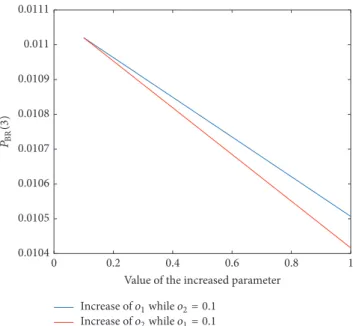
Figure 2:𝑃BR(3)as function of the offer. The blue line illustrates the effect when the offer to the degree 1 depositor is increased while the offer to the degree 2 depositor is kept constant at 0.1, while the red line illustrates the dual case.
In our case the expected costs are as follows:
𝐸 [𝐶 (3)] = 𝑝𝑠(3𝑜22− 2𝑜31+ 6𝑜21− 𝑜32+ 2𝑜12𝛿 + 2𝑜22𝛿
− 2𝑜21𝑝𝑠− 𝑜22𝑝𝑠− 2𝑜21𝛿𝑝𝑠− 2𝑜22𝛿𝑝𝑠) . (12) To fix ideas, we compute the probability of bank run event and the expected costs at𝑡 = 3. Without loss of generality, assume that the probability of being hit by a liquidity shock is 7% and having an impatient neighbor increases by 2.5% the chances that a patient depositor turns impatient as well (𝑝𝑠= 0.07,𝛿 = 0.025) and suppose that𝑓(𝑜deg(𝑖)) = 𝑜deg(𝑖).
Given the payments to depositors with different degree, the probability of bank run event is depicted in Figure 2.
As expected, an increase of the offers implies the decrease of the chance of a bank run event. Second, by increasing the offer to the depositor with the higher degree is more effi- cient. This highlights how important may be to differentiate between depositors regarding the offers.
To determine the optimal strategy of the bank at𝑡 = 3, we have to solve the following nonlinear optimization problem with nonlinear inequality constraints:
min𝑜
1,𝑜2 𝐸 [𝐶 (3)]
subject to 𝑃BR(3) < 𝑃BR. (13) Regarding the above problem, the NLOPT function [13]
of the MATLAB OPTI toolbox was used [14] with the algorithm LDSLSQP. NLOPT was chosen based on its ability of handling nonlinear objective function and constraints, on its numerical stability, and on its advantageous convergence properties. Considering𝛿 = 0.08, the following figures show how the optimal payments and expected cost depend on
10−7 10−6 10−5 10−4 10−3 10−2 10−1 100
c2
0.055 0.06 0.065 0.07 0.075 0.08 0.085 0.09 0.05
ps 0.055 0.06 0.065 0.07 0.075 0.08 0.085 0.09
0.05
ps 10−7
10−6 10−5 10−4 10−3 10−2 10−1 100
c1
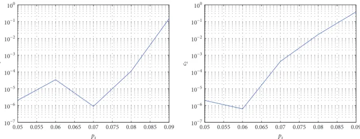
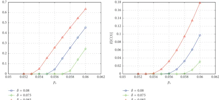
Figure 3: The dependence of optimal offers𝑜opt1 and𝑜opt2 on𝑝𝑠at various levels of𝑃BR.
the model parameters. In these figures we see that if the chance of a liquidity shock (𝑝𝑠) is low enough, the probability of a bank run event remains under the defined threshold even if we offer 0 return to impatient depositors. However, as the probability of becoming impatient (𝑝𝑠) increases, the importance of these offers becomes significant. Furthermore, if we observe the𝑦-axis in the graphs of Figure 3, we see that the optimal offer to a depositor connected to two other depositors is larger, as expected. We defined the function of accepting offer (𝑓) as the identity function, and thus the offered sum is equal to the acceptance probability, so we restrict our analysis to the range where𝑜1, 𝑜2< 1.
Figure 3 shows that the optimal offers to depositors with one and two connected depositors (𝑜opt1 and 𝑜opt2 ) increase as the probability of being hit by a liquidity shock (𝑝𝑠) is increased (as expected) and also shows how the maximum probability of bank run events that the bank admits (𝑃BR) modulates this increase. The larger is the acceptable proba- bility of bank runs, the lower is the offer,ceteris paribus.
Figure 4 shows how the expected cost changes in function of the probability of a liquidity shock (𝑝𝑠) and the acceptable probability of bank run events (𝑃BR). Note that while optimal offers are often almost linear in𝑝𝑠, the expected cost increases nonlinearly in𝑝𝑠.
Finding 1. Anything else held constant, optimal offers increase in the probability of a liquidity shock and in the number of connections. The larger is the probability of bank run event that a bank tolerates, the lower are the optimal offers and hence the expected costs,ceteris paribus.
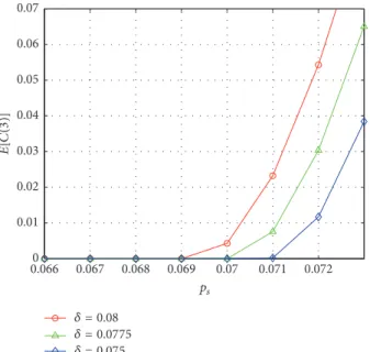
Figures 5 and 6 show how the sensitivity to neighbor depositors who are impatient (𝛿) affects the dependence of the optimal offers (𝑜opt1 ,𝑜opt2 ) and the expected cost (𝐸[𝐶(3)]) on the probability of being hit by a liquidity shock (𝑝𝑠). We assume𝑃BR = 0.02in these cases. As expected, the more an impatient depositor increases the probability of turning impatient of her neighbor(s) (𝛿), the larger is the optimal offer to her so that the probability of bank run event can be kept at the desired level. Note also that the expected cost increases
10−12 10−10 10−8 10−6
E[C(3)]
10−4 10−2 100
0.055 0.06 0.065 0.07 0.075 0.08 0.085 0.09 0.05
ps
Figure 4: The dependence of𝐸[𝐶(3)]on𝑝𝑠at various levels of𝑃BR.
nonlinearly in𝛿as the probability of being hit by a liquidity shock (𝑝𝑠) grows beyond a certain threshold (in our example it is around 0.07).
The interpretation of the bank run event definition may be subject to different considerations. Here we applied a simple approach; however one may define more complex scenarios (e.g., we may consider a state as a bank run if less than half of the depositors is in𝑃state). Such alternative bank run definitions may be easily interpreted in the proposed framework.
The Role of Connections. To get an impression how the connections of the depositors affects the results, we modify the connection structure of Example 1. Now, as depicted in Figure 7, depositor 1 is not connected to depositor 2.
In this case we obtain that
𝑃BR(2) = 𝑝2𝑠(2 − 𝑝𝑠) (2𝛿 + 4𝑝𝑠− 2𝛿𝑝𝑠− 4𝑝𝑠2+ 𝑝𝑠3) , (14)
= 0.08
= 0.0775
= 0.075
= 0.08
= 0.0775
= 0.075
0.067 0.068 0.069 0.07 0.071 0.072 0.066
ps
0 0.1 0.2 0.3 0.4 0.5 0.6
oIJN 2
0.067 0.068 0.069 0.07 0.071 0.072 0.066
ps
0 0.05 0.1 oIJN 1
Figure 5: The dependence of optimal offers𝑜opt1 and𝑜opt2 on𝑝𝑠at various levels of the parameter𝛿, describing the strength of the connections.
= 0.08
= 0.0775
= 0.075 0
0.01 0.02 0.03 0.04 0.05
E[C(3)]
0.06 0.07
0.067 0.068 0.069 0.07 0.071 0.072 0.066
ps
Figure 6: The dependence of𝐸[𝐶(3)]on𝑝𝑠at various levels of the parameter𝛿, describing the strength of the connections.
𝑃BR(3) = 𝑝2𝑠(𝑝𝑠2− 3𝑝𝑠+ 3) (6𝛿 + 9𝑝𝑠− 14𝛿𝑝𝑠− 2𝛿𝑜1 + 10𝛿𝑝𝑠2+ 2𝛿2𝑝𝑠− 2𝛿𝑝3𝑠+ 2𝛿2𝑜1− 2𝛿2− 18𝑝𝑠2 + 15𝑝3𝑠− 6𝑝𝑠4+ 𝑝𝑠5− 2𝛿𝑝2𝑠𝑜1− 2𝛿2𝑝𝑠𝑜1+ 4𝛿𝑝𝑠𝑜1) .
(15)
Moreover,
𝐸 [𝐶 (3)] = 𝑝𝑠(6𝑜12− 𝑜30+ 3𝑜20− 2𝑜31+ 2𝑜21𝛿 − 𝑜20𝑝𝑠
− 2𝑜12𝑝𝑠− 2𝑜21𝛿𝑝𝑠) . (16) Now we have only depositors with zero or one neighbor.
Note that offer to depositors without any connection (𝑜0) does
1
2 3
Figure 7: Topology 2: Connection of the depositors in the case of example2.
not appear in (14) and (15) since an isolated depositor does not affect anybody else. The offer𝑜0does not influence the probability of an isolated depositor changing to𝐼. Once an isolated depositor is in state𝐼, we may enhance her transition to𝑂with a larger𝑜0, but this does not affect the probability of a bank run event. This is the case because an isolated depositor in state𝐼does not influence anybody else, so from the perspective of bank run it does not matter if she is in state 𝐼or𝑂. Trivially, if we want to minimize the expected cost, we choose𝑜0to be zero.
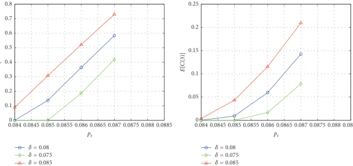
Without loss of generality, we consider the following parameters: 𝛿 = 0.025, 𝑃BR = 0.02. We determine now the optimal offer to depositors with one connection (𝑜1). In Figure 8 we see that, in the case of less connections (i.e., compared to topology 1), a larger 𝑝𝑠 value is required to trigger the role of the offers (about 0.08 instead of about 0.07).
The connection parameter𝛿modulates the results similarly to the previous case depicted in Figure 5. As expected, if the connection structure is sparser (topology 2), the depositors influence each other less, so the expected cost to prevent a bank run is always lower. It reflects the intuitive idea that less connection implies fewer channels to affect other depositors, so the peril of contagion between depositors is more limited.
When there is no connection between depositors, the optimal offer to depositors is zero as we explained before.
In the case when all depositors are connected to each other (topology 3),
= 0.08
= 0.075
= 0.085
= 0.08
= 0.075
= 0.085 0
0.1 0.2 0.3 0.4 0.5 0.6 0.7 0.8
oIJN 1
0.0845 0.085 0.0855 0.086 0.0865 0.087 0.0875 0.088 0.0885 0.084
ps
0 0.05 E[C(3)] 0.150.1 0.2 0.25
0.0845 0.085 0.0855 0.086 0.0865 0.087 0.0875 0.088 0.0885 0.084
ps
Figure 8: The dependence of𝑜opt1 and𝐸[𝐶(3)]on𝑝𝑠and𝛿, in the case of topology 2.
𝑃BR(3) = 54𝛿𝑝𝑠2+ 21𝛿2𝑝𝑠− 180𝛿𝑝3𝑠 − 18𝛿3𝑝𝑠 + 234𝛿𝑝4𝑠+ 3𝛿4𝑝𝑠− 150𝛿𝑝𝑠5+ 48𝛿𝑝𝑠6
− 6𝛿𝑝7𝑠+ 27𝑝3𝑠 − 81𝑝𝑠4+ 108𝑝𝑠5− 81𝑝6𝑠 + 36𝑝𝑠7− 9𝑝𝑠8+ 𝑝9𝑠− 111𝛿2𝑝2𝑠
+ 174𝛿2𝑝3𝑠+ 48𝛿3𝑝2𝑠 − 114𝛿2𝑝𝑠4
− 42𝛿3𝑝3𝑠− 6𝛿4𝑝2𝑠+ 33𝛿2𝑝5𝑠+ 12𝛿3𝑝4𝑠 + 3𝛿4𝑝3𝑠− 3𝛿2𝑝𝑠6− 18𝛿𝑝𝑠2𝑜2− 9𝛿2𝑝𝑠𝑜2 + 54𝛿𝑝3𝑠𝑜2+ 12𝛿3𝑝𝑠𝑜2− 60𝛿𝑝4𝑠𝑜2
− 3𝛿4𝑝𝑠𝑜2+ 30𝛿𝑝5𝑠𝑜2− 6𝛿𝑝𝑠6𝑜2 + 60𝛿2𝑝2𝑠𝑜2− 96𝛿2𝑝3𝑠𝑜2− 36𝛿3𝑝𝑠2𝑜2 + 60𝛿2𝑝4𝑠𝑜2+ 36𝛿3𝑝3𝑠𝑜2+ 6𝛿4𝑝𝑠2𝑜2
− 15𝛿2𝑝5𝑠𝑜2− 12𝛿3𝑝4𝑠𝑜2− 3𝛿4𝑝𝑠3𝑜2,
(17)
𝐸 [𝐶 (3)] = 3𝑜2𝑝𝑠(3 − 𝑝𝑠+ 2𝛿 − 𝑜2− 2𝛿𝑝𝑠) . (18) In Figure 9 we see that, in the case of full connectedness, a lower𝑝𝑠value, compared to the previous cases, is required to trigger the role of the offers (about 0.05), and the expected cost is also higher even in the case of relatively low𝑝𝑠values (compared to Figure 6).
Finding 2. The connection structure between depositors matters. The more connections there are between depositors, the larger are the optimal offers and the expected cost of the bank,ceteris paribus.
3.2. Optimization Problem with Offer Constraints and Time- Dependent Offers. It is a natural to extend the model in a direction which takes into account the bank’s investments, returns, and liquidity, which affects the possible offers.
Moreover, in this section we also allow for the case that the offer changes in time. This is consonant with some papers that we cited before, as, for instance, [2, 3] also show that banks adjust the payments to the new situations. However, we assume that the bank does not reevaluate the situation between time periods (in this case the realized states could be taken into account as certain starting state of the model, and the optimization could be performed according to this), all offers are determined prior. While these features make the model more realistic, they make it more complicated also. Hence, in this section we focus on the example that we introduced in the last section.
Consider again the topology depicted in Figure 1 and a time horizon of 4 periods. The state transition matrix𝑄will be time-dependent, since the offers at𝑡 = 1and𝑡 = 2may differ. We denote the offer to a depositor with𝑛neighbors at time𝑡as𝑜𝑛(𝑡).
Since the offers (𝑜𝑛) are time-dependent, the resulting values of the acceptance functions (𝑓(𝑜𝑛(𝑡))) are also time dependent. We assume that they are the same for all deposi- tors with the same degree.
Since the main risk is to leave depositors too long in the impatient state, we expect that earlier offers should be larger.
On the other hand early offers are limited by early returns. In the optimization problem below we take this consideration into account.
In this case the probability of bank run event at𝑡 = 3is
𝑃BR(3) = 36𝛿𝑝𝑠2+ 7𝛿2𝑝𝑠− 120𝛿𝑝3𝑠− 4𝛿3𝑝𝑠+ 156𝛿𝑝𝑠4 + 𝛿4𝑝𝑠− 100𝛿𝑝5𝑠 + 32𝛿𝑝6𝑠 − 4𝛿𝑝7𝑠 + 27𝑝𝑠3
= 0.08
= 0.075
= 0.085
= 0.08
= 0.075
= 0.085
0.052 0.054 0.056 0.058 0.06 0.062
0.05
ps
0 0.02 0.04 0.06 0.08 0.1
E[C(3)]
0.12 0.14 0.16 0.18
0.052 0.054 0.056 0.058 0.06 0.062
0.05
ps
0 0.1 0.2 0.3 0.4 0.5 0.6 0.7
oIJN 2
Figure 9: The dependence of𝑜opt2 and𝐸[𝐶(3)]on𝑝𝑠and𝛿, in the case of topology 3 (full connectedness).
− 81𝑝𝑠4+ 108𝑝5𝑠− 81𝑝𝑠6+ 36𝑝7𝑠− 9𝑝8𝑠 + 𝑝𝑠9
− 43𝛿2𝑝2𝑠+ 70𝛿2𝑝3𝑠+ 12𝛿3𝑝2𝑠− 46𝛿2𝑝4𝑠
− 12𝛿3𝑝3𝑠− 2𝛿4𝑝2𝑠+ 13𝛿2𝑝5𝑠+ 4𝛿3𝑝𝑠4 + 𝛿4𝑝𝑠3− 𝛿2𝑝6𝑠 − 6𝛿𝑝2𝑠𝑓 (𝑜1(1))
− 6𝛿𝑝𝑠2𝑓 (𝑜2(1)) + 18𝛿𝑝3𝑠𝑓 (𝑜1(1))
− 3𝛿2𝑝𝑠𝑓 (𝑜2(1)) + 18𝛿𝑝𝑠3𝑓 (𝑜2(1))
− 20𝛿𝑝4𝑠𝑓 (𝑜1(1)) + 4𝛿3𝑝𝑠𝑓 (𝑜2(1))
− 20𝛿𝑝4𝑠𝑓 (𝑜2(1)) + 10𝛿𝑝5𝑠𝑓 (𝑜1(1))
− 𝛿4𝑝𝑠𝑓 (𝑜2(1)) + 10𝛿𝑝𝑠5𝑓 (𝑜2(1))
− 2𝛿𝑝𝑠6𝑓 (𝑜1(1)) − 2𝛿𝑝6𝑠𝑓 (𝑜2(1)) + 8𝛿2𝑝2𝑠𝑓 (𝑜1(1)) + 18𝛿2𝑝2𝑠𝑓 (𝑜2(1))
− 14𝛿2𝑝3𝑠𝑓 (𝑜1(1)) − 30𝛿2𝑝3𝑠𝑓 (𝑜2(1)) + 8𝛿2𝑝4𝑠𝑓 (𝑜1(1)) − 12𝛿3𝑝2𝑠𝑓 (𝑜2(1)) + 20𝛿2𝑝4𝑠𝑓 (𝑜2(1)) − 2𝛿2𝑝5𝑠𝑓 (𝑜1(1)) + 12𝛿3𝑝3𝑠𝑓 (𝑜2(1)) + 2𝛿4𝑝2𝑠𝑓 (𝑜2(1))
− 5𝛿2𝑝5𝑠𝑓 (𝑜2(1)) − 4𝛿3𝑝4𝑠𝑓 (𝑜2(1))
− 𝛿4𝑝𝑠3𝑓 (𝑜2(1)) ;
(19) the above expression (19) is a slight modification of (11).
𝑃BR(4), which depends also on𝑓(𝑜1(2))and𝑓(𝑜2(2)), can be similarly derived; however the expression is too long to be detailed here.
Regarding the expected cost, the derivation is not as simple as in Section 3.1, since if a state ends up in𝑂, it does matter when did it change from𝐼to𝑂. As detailed earlier, the offers in𝑡 = 3do not affect the probability of the bank run event at𝑡 = 4, so it is enough to derive the expected costs of the states at𝑡 = 3.Consider a simple example. The expected cost of the state𝑃𝑂𝑂at time𝑡 = 3may be calculated as
𝑝12(3) (𝑝5(2) (2𝑜1(2)) + 𝑝22(2) (𝑜1(1) + 𝑜1(2)) + 𝑝23(2) (𝑜1(1) + 𝑜1(2)) + 𝑝12(2) (2𝑜1(1))) , (20) where𝑝12(3)is the probability of state 12 at time𝑡 = 3and so on. Let us discuss this expression a bit more in detail. The expected cost of state𝑃𝑂𝑂at𝑡 = 3 is proportional to its probability 𝑝12(3). Furthermore there are 4 ways to get to 𝑃𝑂𝑂 = 𝜎12:
(i) From𝑃𝐼𝐼 = 𝜎5: in this case both depositor 2 and depositor 3 (depositors with one neighbor) accept the offer at 𝑡 = 2, so the relevant term is 𝑝5(2𝑜1(2)) (remember that𝑜1(2)refers to offers with one neigh- bor at time𝑡 = 2).
(ii) From𝑃𝐼𝑂 = 𝜎22: in this case depositor 3 accepted the offer at𝑡 = 1(since he is already in𝑂state), while depositor 2 accepted the offer at𝑡 = 2which implies 𝑝22(𝑜1(1) + 𝑜1(2)).
(iii) From𝑃𝑂𝐼 = 𝜎23: in this case depositor 3 accepted the offer at𝑡 = 2, while depositor 2 accepted the offer at 𝑡 = 1which implies𝑝23(𝑜1(1) + 𝑜1(2)).
(iv) From𝑃𝑂𝑂 = 𝜎12: in this case both depositors 2 and 3 accepted the offer at𝑡 = 1:𝑝12(2𝑜1(1)).
With the summation of all such expressions we can derive the expression for the expected cost at𝑡 = 3.