1
Habitat heterogeneity as a key to high conservation value in forest-grassland mosaics 1
2
Abstract 3
4
Forest-grassland mosaics are widespread features at the interface between tree- and grass- 5
dominated ecosystems. However, the importance of habitat heterogeneity in these mosaics is 6
not fully appreciated, and the contribution of individual woody and herbaceous habitats to the 7
overall conservation value of the mosaic is unclear. We distinguished six main habitats in the 8
forest-grassland mosaics of the Kiskunság Sand Ridge (Hungary) and compared the species 9
composition, species richness, Shannon diversity, naturalness, selected structural features, 10
environmental variables, and the number of protected, endemic, red-listed and specialist 11
species of the plant communities. Each habitat had species that were absent or rare elsewhere.
12
Grasslands had the highest conservation importance in most respects. North-facing forest 13
edges had the highest species richness, while south-facing edges were primarily important for 14
tree recruitment. Among the forest habitats, small forest patches were the most valuable, 15
while large and medium forest patches had the lowest conservation importance. We showed 16
that the current single-habitat focus of both research and conservation in the studied forest- 17
grassland mosaics is not justified. Instead, an integrated view of the entire mosaic is 18
necessary. Management practices and restoration projects should promote habitat 19
heterogeneity, e.g., by assisting tree and shrub establishment and survival in grasslands. The 20
legislative background should recognize the existence of fine-scale forest-grassland mosaics, 21
which are neither grasslands nor forests, but a mixture.
22 23
Keywords: Complexity, Conservation management, Forest edge, Forest patches, Forest- 24
steppe, Landscape heterogeneity 25
26
1. Introduction 27
28
The intensification of land-use practices and the resulting habitat homogenization pose 29
major challenges for current conservation (Ernst et al., 2017; Foley et al., 2005; Rembold et 30
al., 2017; Stoate et al., 2001). Likewise, land abandonment often leads to homogenization 31
(Bergmeier et al., 2010; Plieninger et al., 2015; Ernst et al. 2017). Generally, heterogeneous 32
areas are expected to contain more niches and, consequently, more species than homogeneous 33
areas (Bazzaz, 1975; Chesson, 2000; Tilman, 1982). In fact, spatial heterogeneity seems 34
necessary for the maintenance of biodiversity, ecosystem services, and endangered species 35
(Armengot et al., 2012; Dorresteijn et al., 2015; Valkó et al., 2012). Thus, from a 36
conservation perspective, the presence of various habitat patches in close proximity is 37
considered beneficial (Jakobsson and Lindborg, 2015; Tölgyesi et al., 2017).
38
Habitat heterogeneity and its conservation implications are relatively well studied in 39
agricultural and agroforestry landscapes (e.g., Bennett et al., 2006; Benton et al., 2003;
40
Jakobsson and Lindborg, 2015; Lee and Martin, 2017; Manning et al., 2006; Moreno et al., 41
2017; Plieninger et al., 2015; Stoate et al., 2001; Tscharntke et al., 2005). Unfortunately, the 42
importance of habitat heterogeneity for conservation has received less attention in natural 43
mosaics at the interfaces of tree- and grass-dominated biomes (cf. Tews et al., 2004).
44
Forest-grassland mosaics typically consist of numerous types of forest and grassland 45
patches of various sizes, as well as intervening edge communities, with strongly different 46
physiognomies and environmental conditions (Breshears, 2006; Schultz, 2005). In such 47
mosaics, appropriate conservation actions and adequate management strategies require an 48
integrated view of the complex ecosystem (Luza et al., 2014).
49
2
Forest-grassland mosaics represent high conservation significance (Erdős et al., 2018;
50
Prevedello et al., 2018). However, in Eastern Europe, most of these mosaics have been 51
transformed to croplands or non-native tree plantations, while the remaining fragments are 52
threatened by different forms of homogenization (Wesche et al., 2016). In some regions, the 53
spontaneous or human-induced spread of woody species may result in the disappearance of 54
grassland habitats. At the same time, woody habitats are diminishing in other regions due to 55
the combined effects of climate change, sinking groundwater level, and fire (Molnár, 1998;
56
Wesche et al., 2016).
57
The conservation importance of habitat heterogeneity in the natural forest-grassland 58
mosaics of Eastern Europe is, as yet, not fully appreciated. Ecological studies have typically 59
focused on either the grassland or the forest component separately, disregarding the mosaic 60
character (Erdős et al., 2015). The same bias exists in conservation practice. For example, 61
restoration efforts usually aim to reconstruct only one of the components (e.g., Filatova and 62
Zolotukhin, 2002; Halassy et al., 2016; Szitár et al., 2016; Török et al., 2014). Projects that 63
intend to restore entire mosaic complexes (i.e., both woody and herbaceous components) are 64
scarce (Török et al., 2017). While grazing and mowing are traditional and effective tools in 65
both restoration and conservation management, changes in land-use in the form of either 66
intensification (e.g., overgrazing, mechanized mowing) or abandonment may reduce 67
heterogeneity and may thus have a detrimental effect on these complex systems (Bergmeier et 68
al., 2010; Öllerer, 2014; Tölgyesi et al., 2017).
69
In this study, our aim was to explore the contribution of individual woody and 70
herbaceous habitats to the overall conservation value of the entire mosaic. Our questions were 71
the following: (1) If we aim to protect the entire species pool of the mosaic, is it sufficient to 72
conserve one or a few keystone habitats, or is it necessary to conserve all of them? (2) What is 73
the importance of individual habitats in terms of conservation-related characteristics (species 74
richness, diversity, the number of species with special conservation relevance, naturalness, 75
tree size-classes and recruitment, adventives)? (3) How does environmental heterogeneity 76
support the observed vegetation pattern?
77 78
2. Material and methods 79
80
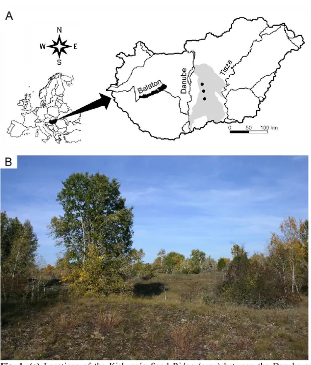
2.1. Study area 81
The study was conducted in the Kiskunság Sand Ridge, which is a lowland area 82
between the Danube and Tisza rivers in Hungary. Three study sites were selected:
83
Tatárszentgyörgy (N 47°02’, E 19°22’), Fülöpháza (N 46°52’, E 19°25’), and Bócsa (N 84
46°41’, E 19°27’) (Fig. 1a). All three sites are part of the Natura 2000 network of protected 85
areas, and the Fülöpháza and Bócsa sites belong to the Kiskunság National Park. The mean 86
annual temperature is 10.3-10.5 °C, and the mean annual precipitation is 520-550 mm 87
(Tölgyesi et al., 2016). The study sites are characterized by stabilized calcareous sand dunes 88
and interdune depressions that are covered by humus-poor sandy soils with low water 89
retention capacities (Várallyay, 1993).
90
The vegetation is a mosaic of woody and herbaceous components (Fig. 1b). The open 91
perennial sand grassland (Festucetum vaginatae, Natura 2000 category: 6260, *Pannonic sand 92
steppes, a habitat of community importance in the European Union) is the most widespread 93
natural herbaceous community of the study sites. The total cover of vascular plants usually 94
varies between 40 and 70%, and the rest of the area is covered by mosses, lichens, or bare 95
sand. The dominant species are Festuca vaginata, Stipa borysthenica, and S. capillata, while 96
Alkanna tinctoria, Dianthus serotinus, Euphorbia segueriana, Fumana procumbens, and Poa 97
bulbosa are also common.
98
3
Patches of the juniper-poplar forest (Junipero-Populetum albae, Natura 2000 category:
99
91N0, Pannonic inland sand dune thicket) are scattered in the grassland. The canopy layer has 100
a cover of 40-60% and is co-dominated by 10-15 m tall Populus alba and P. × canescens 101
individuals. The shrub layer cover varies between 5 and 80% with heights of 1-5 m, and is 102
composed of Berberis vulgaris, Crataegus monogyna, Juniperus communis, and Ligustrum 103
vulgare. The most common species in the herb layer include Anthriscus cerefolium, 104
Asparagus officinalis, Carex liparicarpos, Cynoglossum officinale, Poa angustifolia, and tree 105
and shrub seedlings. Some xeric species, such as Eryngium campestre, Festuca rupicola, and 106
Potentilla arenaria, are mainly found under canopy gaps. The sizes of the forest patches 107
range from a few individual trees (approx. 50 m2) to a few hectares, although patches larger 108
than 1 ha are rare.
109
The study sites were extensively grazed till the end of the 19th century. In the 20th 110
century, the Fülöpháza and the Bócsa sites were used for military exercises, which stopped in 111
1974 (Biró et al., 2013; Kertész et al., 2017). Currently the level of anthropogenic 112
disturbances is very low (strictly regulated tourism and research). There is strong evidence 113
that the mosaic character is a result of climatic features and soil characteristics, and the 114
grassland component persists even without grazing or other forms of disturbances 115
(Bodrogközy, 1982; Erdős et al., 2015; Fekete, 1992). Both the position and the extent of the 116
studied habitat patches are relatively stable at a decadal time-scale: grassland-to-forest or 117
forest-to-grassland transitions are rare and occur very slowly (Erdős et al., 2015; Fekete, 118
1992).
119 120
2.2. Sampling design 121
Based on previous research (Erdős et al., 2015), six habitat types were distinguished in 122
the present study: large forest patches (> 0.5 ha), medium forest patches (0.2-0.4 ha), small 123
forest patches (< 0.1 ha), north-facing forest edges, south-facing forest edges, and grasslands.
124
Patches were selected randomly for the study. Plots within the individual patches were placed 125
so as to ensure representativeness and avoid degraded areas such as road or path margins and 126
plantations. Edge plots were established in more or less straight peripheral zones of forest 127
patches > 0.2 ha outward from the outermost tree trunks but still under the canopy. We 128
sampled a total of 90 permanent plots (3 sites × 6 habitats × 5 replicates). Plot size was 25 m2 129
(2 m × 12.5 m at edges, 5 m × 5 m elsewhere). The sizes and shapes of the plots were 130
determined according to the local circumstances: the size was small enough to sample even 131
the smallest forest patches but large enough for a standard coenological relevé, whereas the 132
elongated form of the edge plots ensured that they did not extend into the forest or grassland 133
interiors.
134
Within each plot, the percent covers of all vascular plant species in all vegetation 135
layers were visually estimated in April (spring aspect) and July (summer aspect) 2016. Visual 136
estimations were done by the same person in all plots. Of the spring and summer cover 137
values, for each species, the largest value was used for subsequent data analyses.
138
All individual trees were inventoried in the plots, and the diameter at breast height 139
(DBH) was measured for trees taller than 1.3 m.
140
As potential environmental drivers of vegetation in the different habitats, microclimate 141
variables and soil moisture content were measured in 30 plots (6 habitats × 5 replicates) at the 142
Fülöpháza site. Among the three study sites, Fülöpháza lies in the middle, in an almost equal 143
distance from the other two sites. Air temperature (°C) and relative air humidity (%) were 144
measured synchronously for 24 hours at 25 cm above the ground surface in the centre of each 145
plot using MCC USB-502 data loggers (Measurement Computing Corp). Microclimate 146
loggers were housed in naturally ventilated radiation shields to avoid direct solar radiation, 147
4
and the logging interval was set to 1 min. Measurements occurred from 3 to 4 August under 148
clear weather conditions. Soil moisture values were measured in the upper 20 cm layer on 26 149
July using a FieldScout TDR300 Soil Moisture Meter (Spectrum Technologies Inc). Five 150
measurements were carried out for each plot, which were then averaged.
151 152
2.3. Data analyses 153
To assess the compositional relations of the six habitat types, we performed a non- 154
metric multidimensional scaling (NMDS) using Bray-Curtis distance on the square root 155
transformed cover scores. We conducted the analysis with one to six axes and found that 156
using three or more axes caused only slight and linear decreases of the stress factors compared 157
with the two-dimensional solution, so we decided to use only two axes. The analysis was 158
performed in R 3.4.3 (R Core Team, 2017) using the ‘metaMDS’ function of the vegan 159
package (Oksanen et al., 2016).
160
To identify the species that prefer one specific habitat type and are absent or rare in 161
other habitats, we performed a diagnostic species analysis. The phi coefficient was applied as 162
an indicator of the fidelity of a species to certain habitats (Chytrý et al., 2002). The phi 163
coefficient varies between -1 and +1; higher values reflect higher diagnostic values. In this 164
study, species with phi values > 0.200 were considered. Significant (P < 0.01) diagnostic 165
species were identified by applying Fisher’s exact test. Analyses were performed with JUICE 166
7.0.45 (Tichý, 2002).
167
Species richness and Shannon diversity were computed for each plot, and the per plot 168
number of species with special conservation relevance was also enumerated, which included 169
all protected, endemic, red-listed and specialist species and was based on Borhidi (1995), 170
Király (2007), and the Database of Hungarian Natural Values (www.termeszetvedelem.hu).
171
As a numeric descriptor of habitat naturalness, we used the relative naturalness indicator 172
values of Borhidi (1995), defined for the Hungarian flora. Naturalness indicator values are 173
defined along an ordinal scale and reflect the observed tolerances of species against habitat 174
degradation. Species that tend to be related to natural habitats have higher values, while 175
species that are more frequent in degraded sites have lower values. Despite some criticism, 176
bio-indication in general and naturalness indicators in particular have solid theoretical bases 177
and obvious practical advantages (Diekmann, 2003). Earlier analyses have shown that mean 178
naturalness values are able to indicate habitat naturalness/degradation (Erdős et al., 2017;
179
Sengl et al., 2016, 2017). Here, we calculated the unweighted mean value for each plot, as it is 180
more efficient in site indication than cover-weighted approaches (Tölgyesi et al., 2014).
181
The species richness, Shannon diversity, number of species with special conservation 182
relevance, and naturalness values were analysed in the R environment with linear mixed- 183
effects models. Site was included as the random factor and habitat was the fixed factor. We 184
used a Poisson error term for the count data (species richness and the number of species with 185
special conservation relevance) and assumed a Gaussian distribution for the continuous 186
variables (Shannon diversity and mean naturalness value). We used the ‘glmer’ function of 187
the lme4 package (Bates et al., 2015) for the former situation, and the ‘lme’ function of the 188
nlme package (Pinheiro et al., 2016) for the latter one. The full models were tested for 189
significance with analysis of variance, and if the model explained a significant proportion of 190
the variability, we considered pairwise comparisons of the levels of the fixed factor. To 191
account for multiple comparisons, we adjusted the resulting P values with the false discovery 192
rate (FDR) method.
193
The size-class distribution of the trees was studied using 5 cm diameter classes. The 194
distributions were compared with the Kolmogorov-Smirnov test. Stand characteristics, such 195
as the mean and maximum DBH and number of trees per ha, were calculated for both native 196
5
and adventive species. The nativeness or adventiveness of the tree species was defined 197
according to Király (2009), as shown in Table A1.
198
Using the collected microclimate data, we calculated the following variables: mean 199
daily air temperature, mean daytime air temperature, mean nighttime air temperature, mean 200
daily relative air humidity, mean daytime relative air humidity, and mean nighttime relative 201
air humidity. Daytime was defined here as the interval from 7:01 a.m. to 7:00 p.m., while 202
nighttime was the interval from 7:01 p.m. to 7:00 a.m.
203
To assess the relationships between environmental variables and vegetation pattern, 204
we conducted a distance-based redundancy analysis (dbRDA) in the R environment using the 205
‘capscale’ function of the vegan package (Oksanen et al., 2016). The ordination was 206
performed using Bray-Curtis distance on the square root transformed species cover scores.
207
For a preliminary dbRDA model, we included seven environmental variables (all six 208
microclimatic variables mentioned above, and soil moisture) and calculated the variance 209
inflation factor (VIF) of each variable to check for multicollinearity. We then removed the 210
variable with the highest VIF and recreated the model. We continued this step-by-step 211
refinement until every VIF was less than five. Finally, we retained only daily mean 212
temperature, nighttime mean temperature, daily mean relative humidity, and mean soil 213
moisture. To find the best model using any of these four explanatory variables, we used the 214
forward selection method (‘ordistep’ function). We tested the final dbRDA model and the 215
effect of each explanatory variable for significance with analysis of variance using 1000 216
permutations each.
217
The plant species names follow Király (2009), while the plant community names are 218
according to Borhidi et al. (2012).
219 220
3. Results 221
222
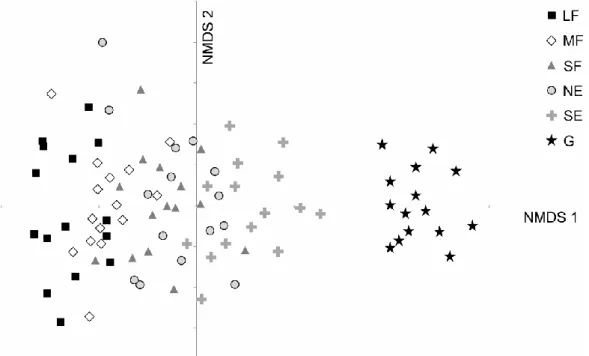
We found a total of 182 plant species in the 90 plots. The NMDS ordination indicated 223
a well-defined gradient in the following sequence: large forest patches – medium forest 224
patches – small forest patches and north-facing edges – south-facing edges – grasslands (Fig.
225
2). Most groups overlapped considerably (especially small forest patches and north-facing 226
edges), but grasslands were distinct from the other habitats.
227
The significant (P < 0.01) diagnostic species of the six habitats are shown in Table A2.
228
Large forest patches had seven diagnostic species, mostly native shrubs (e.g., Cornus 229
sanguinea, Prunus spinosa). Two native shrubs (Crataegus monogyna, Berberis vulgaris) 230
were identified as diagnostic species for medium forest patches. Seven species were 231
significantly associated with small forest patches, most of which were herbs (e.g., Solanum 232
dulcamara, Eryngium campestre). North-facing edges had ten diagnostic species (e.g., 233
Carlina vulgaris, Polygala comosa). South-facing edges also had ten diagnostic species (e.g., 234
Koeleria glauca, Poa bulbosa), of which they shared four species with the grassland habitat.
235
Twenty species were associated with grasslands (e.g., Alkanna tinctoria, Fumana 236
procumbens).
237
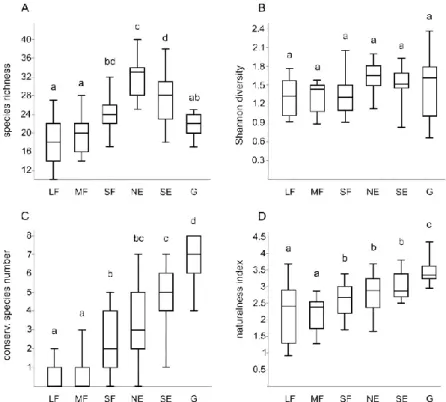
Habitat type had significant effects on species richness (χ2 = 70.62, P < 0.001), 238
Shannon diversity (χ2 = 12.31, P = 0.031), the number of species with special conservation 239
relevance (χ2 = 129.16, P < 0.001), and the mean naturalness value (χ2 = 70.84, P < 0.001).
240
Considering the pairwise comparisons (Table A3), north-facing edges had the highest species 241
richness followed by south-facing edges (Fig. 3a). Species richness was lowest in large and 242
medium forest patches, while grasslands and small forest patches had intermediate species 243
richness. There were no significant differences among the Shannon diversities of the different 244
habitats, although north-facing edges and south-facing edges seemed to have somewhat 245
6
higher Shannon diversity values than large, medium, and small forest patches (Fig. 3b). These 246
differences were significant in only the uncorrected set of P values. The number of species 247
with special conservation relevance showed a gradually increasing trend from the large forest 248
patches towards the grasslands (Fig. 3c). A similar pattern was detected for the mean 249
naturalness values (Fig. 3d).
250
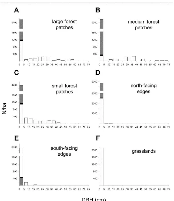
Recruitment of native trees (mainly Populus alba and P. × canescens, to a much lesser 251
degree Quercus robur) seemed to occur in mainly the south-facing edges and to a lesser 252
degree in the north-facing edges and grasslands (Fig. 4, Table 1). In contrast, the recruitment 253
of adventive trees (e.g., Ailanthus altissima, Celtis occidentalis, Padus serotina, and Robinia 254
pseudoacacia) was concentrated in the forest interiors of all patch sizes and north-facing 255
edges, while it was rare in the south-facing edges and completely absent in grasslands. The 256
numbers of larger native trees (DBH > 5 cm) were almost equal in large, medium, and small 257
forest patches, while adventive trees with DBH > 5 cm were present in only large forest 258
patches. Large native trees (DBH > 50 cm) were present in mainly large and medium forest 259
patches and to a lesser degree in small forest patches. Adventive tree species were not able to 260
develop to large sizes in any of the studied habitats. According to the Kolmogorov-Smirnov 261
tests (Table 2), the six habitats formed two groups: large, medium, and small forest patches 262
were similar to one another, but differed significantly from the other three habitats (north- 263
facing edges, south-facing edges, and grasslands).
264
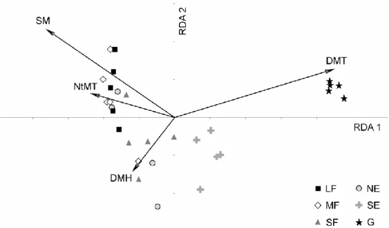
The results of the environmental measurements are shown in Table A4. The best 265
dbRDA model contained all four explanatory variables that were retained (daily mean 266
temperature, nighttime mean temperature, daily mean relative humidity, and soil moisture), 267
and it was significant (R2 = 0.276, F = 3.76, P < 0.001). Although three of the variables were 268
retained during variable selection, they had nonsignificant effects (nighttime mean 269
temperature: F = 1.28, P = 0.214, daily mean humidity: F = 0.98, P = 0.394, and soil 270
moisture: F = 1.67, P = 0.099), and only daily mean temperature had a significant effect 271
(F = 2.81, P = 0.019). The dbRDA biplot (Fig. 5) indicated that woody (forest and edge) and 272
non-woody (grassland) habitats were separated according to daily mean temperature, with 273
higher values pointing towards the grassland. Interestingly, soil moisture, although having 274
only a marginally significant effect, explained the distribution of the woody habitat types in 275
the ordination space.
276 277
4. Discussion 278
279
4.1. Compositional differences among habitats 280
The composition of the studied habitats formed a gradient from large forest patches to 281
grasslands. However, species turnover was not continuous, and two well-defined groups 282
emerged. The first group contained the grassland habitat, which had the most distinct species 283
composition and the highest number of diagnostic species, suggesting that the grassland 284
species pool is poorly represented in other habitats. The second group consisted of all other 285
(woody) habitats with partly overlapping species compositions and fewer diagnostic species.
286
This most basic distinction (woody vs. herbaceous habitats) defines the minimum 287
conservation requirement in the studied ecosystem: To represent a considerable proportion of 288
the species pool of the landscape, it is necessary to preserve both the grassland and at least 289
some of the woody habitats.
290
Given its relatively large variation, the woody habitat group may be further subdivided 291
into edge-like habitats (small forest patches, north-facing edges, and south-facing edges) and 292
forests with core areas (large forest patches and medium forest patches). To achieve a higher 293
landscape-level diversity, it is recommended to conserve at least some edge-like habitats and 294
7
some forest patches with core areas. However, our results emphasize that all six habitats have 295
their typical species composition and species that are significantly concentrated within each of 296
them. Thus, all habitats deserve special consideration in conservation policy and practice if 297
we aim to protect the highest possible proportion of the species pool.
298
Until very recently, between-habitat compositional differences have received 299
surprisingly little attention in Eastern European forest-grassland mosaics, where conservation 300
efforts usually focus on only the grassland component (Erdős et al., 2013). In line with the 301
results of Bátori et al. (2018), Kelemen et al. (2017) and Tölgyesi et al. (2017), our study 302
revealed low redundancy between the woody and herbaceous components, which calls for 303
increased efforts to conserve forest habitats in the studied ecosystem.
304 305
4.2. Conservation-related characteristics of the habitats 306
One of our most important findings was that the six habitats in the studied ecosystem 307
had strongly different conservation-related characteristics. Grasslands had the highest per plot 308
number of species with special conservation relevance (protected, endemic, red-listed, and 309
specialist species). Similarly, in a mosaic of oak forests and xeric grasslands, Molnár (1998) 310
found that grasslands contained more specialist species than either forest interiors or forest 311
edges. Our results show that the grassland habitat had the highest naturalness. In addition, 312
adventive tree seedlings were completely absent from grasslands, which is in good agreement 313
with earlier studies that indicated low invasibility of undisturbed sand grasslands in the region 314
(Bagi, 2008; Csecserits et al., 2016; Szigetvári, 2002). The conservation importance of the 315
grassland habitat is probably further enhanced by other taxa that were not analysed in this 316
study. For example, sandy grasslands are rich in mosses and lichens, including the endemic 317
species Cladonia magyarica (Borhidi et al., 2012).
318
In our study, edges (especially north-facing ones) had the highest species richness, 319
which is in line with the edge-effect theory (Risser, 1995). Similarly, forest edges were 320
proven to be quite species-rich in other natural and near-natural mosaics in Eastern Europe 321
(Erdős et al., 2013; Molnár, 1998), Asia (Bátori et al., 2018), and South America (de 322
Casenave et al., 1995; Pinder and Rosso, 1998). In addition to hosting high fine-scale species 323
richness, edges play an important role in tree recruitment: The number of native tree seedlings 324
and saplings was the highest in south-facing edges, but it was also considerable in north- 325
facing ones. Thus, forest edges may play a crucial role in the dynamics of forest-grassland 326
mosaics (Erdős et al., 2015).
327
Forest patches of different sizes may be substantially dissimilar in several respects, 328
although most earlier studies have been conducted in anthropogenic mosaics (e.g., Carranza et 329
al., 2012; Gignac and Dale, 2007; Kolb and Diekmann, 2005; Rosati et al., 2010). In the fine- 330
scale natural mosaics of Hungary, forest patches are usually very small (typically up to a few 331
hectares) (Wesche et al., 2016). The small range of forest patch sizes may explain why forest 332
patches of different sizes have received little attention. Interestingly, despite this small 333
variation in size (the lower threshold of the large forest category was only 0.5 ha in our 334
study), considerable differences were found among small forest patches on the one hand, and 335
medium and large forest patches on the other.
336
Small forest patches had significantly higher species richness, more species of special 337
conservation interest, and higher naturalness than large and medium forest patches. The 338
differences in stand characteristics were less pronounced, although the number of large trees 339
(DBH > 50 cm) in small forests was low compared to the numbers in medium and large forest 340
patches. Medium and large forest patches had low species richness, only a few species of 341
special conservation relevance, and low naturalness values. In addition, large and medium 342
forest patches hosted the largest proportions of adventive trees; thus, these forests should be 343
8
regarded as potential invasion hot-spots. Csecserits et al. (2016) identified the following 344
habitats as invasion hot-spots in our study region: tree plantations, agricultural habitats, old- 345
fields, and oak forests. Pándi et al. (2014) concluded that abandoned farms are invasion 346
centres. From these sources, adventive species with good dispersal abilities can easily reach 347
all six habitat types evaluated in this study, but they probably have the best establishment 348
chances in relatively humid and cool habitats such as medium and large forest patches.
349
Medium and large forest patches seemed to have relatively low conservation 350
importance. However, they added structural characteristics to the landscape that small forest 351
patches lacked. The noticeable number of native shrubs and large trees (DBH > 50 cm) should 352
be considered important from a conservation perspective. For example, large trees provide 353
habitat for several protected animals, including insects (e.g., Aegosoma scabricorne and 354
Oryctes nasicornis) and birds (e.g., Coracias garrulus and other cavity-nesting birds) (Foit et 355
al., 2016; Gaskó, 2009). It should also be kept in mind that the existence of edges depends on 356
forest patches of sufficient size.
357 358
4.3. Environmental heterogeneity 359
Environmental parameters are expected to differ between woody and herbaceous 360
patches in mosaic ecosystems (e.g., Breshears, 2006; Schmidt et al., 2017). In our study, the 361
daily mean temperature differed significantly between woody and herbaceous habitats, while 362
soil moisture showed conspicuous differences among the different woody habitats. Although 363
the causal relations between vegetation and the environment are complex, it may be assumed 364
that trees modify their environment in a way that has a profound effect on the herb layer (cf.
365
Scholes and Archer, 1997). This moderating effect is expected to be especially strong in harsh 366
environments (Callaway and Walker, 1997) such as the semi-arid Kiskunság Sand Ridge.
367
Soil moisture and daily mean and daytime mean air humidity were higher in the forest 368
patches than in the grasslands, while the daily mean and daytime mean temperature were 369
lower, and the maxima and minima of both temperature and humidity were less extreme in the 370
forest patches. Thus, conserving woody habitats is important for creating environments that 371
are suitable for mesic plants that would be unable to survive in the dry grassland component 372
of the mosaic. This role of trees and groves is predicted to become increasingly important 373
with ongoing climate change (Manning et al., 2009).
374 375
4.4. Conclusions and implications for conservation policy and practice 376
Our study implies that maintaining habitat heterogeneity through the protection of 377
various habitats is of crucial conservation importance. Some habitats have outstanding species 378
richness, some possess high resistance against invasion, and others are important mainly for 379
tree recruitment or structural reasons. In addition, all habitats have characteristic species 380
compositions with species that are absent or rare elsewhere.
381
In concordance with the findings of Török et al. (2017) and Weking et al. (2016), our 382
study suggests that it is not sufficient to focus on either the grassland or the forest components 383
in conservation-oriented research and practice. Rather, an integrated view of the entire mosaic 384
is urgently needed. For example, the establishment of native trees should be promoted in areas 385
where they have been reduced through cutting, overgrazing or fire (e.g., by deploying safe 386
sites for seedlings). Management practices should be adapted to support native tree 387
recruitment (e.g., by decreasing grazing pressure). During restoration projects, the 388
reconstruction of forest patches should be of high priority.
389
Inappropriate legislation is a possible explanation why the complexity of forest- 390
grassland mosaics has been neglected in both research and management in Eastern Europe 391
(Babai et al., 2015; Hartel et al., 2013; Korotchenko and Peregrym, 2012; Tölgyesi et al., 392
9
2017; Varga et al., 2016). From a legal perspective, an area may be treated as either forest or 393
grassland, but not as a mosaic of both. These two categories (i.e., forest and grassland) do not 394
match reality in Eastern Europe, where the natural vegetation of large areas is actually a 395
mosaic of woody and herbaceous patches.
396
Adapting conservation policy and practice to fit the complexity of forest-grassland 397
mosaics may be a difficult task; however, there is no alternative if the natural values of these 398
unique ecosystems are to be conserved.
399 400
Statement of competing interests 401
The authors have no competing interests to declare.
402 403
Funding sources and acknowledgements 404
Funding: This work was supported by the Hungarian Scientific Research Fund [grant 405
number OTKA PD 116114]; the National Youth Excellence Program [grant number NTP- 406
NFTÖ-16-0623]; and the National Research, Development and Innovation Office [grant 407
number NKFIH K 124796]. The funding sources played no role in study design and research 408
conduct. We are thankful to Dolly Tolnay and Mihály Szőke-Tóth for their help with the field 409
work and data analyses.
410 411
References
412 Armengot, L., Sans, F.X., Fischer, C., Flohre, A., José‐María, L., Tscharntke, T., Thies, C., 413 2012. The β‐diversity of arable weed communities on organic and conventional cereal 414
farms in two contrasting regions. Appl. Veg. Sci. 15, 571–579.
415
Babai, D., Tóth, A., Szentirmai, I., Biró, M., Máté, A., Demeter, L., Szépligeti, M., Varga, A., 416
Molnár, Á., Kun, R., Molnár, Zs., 2015. Do conservation and agri-environmental 417
regulations effectively support traditional small-scale farming in East-Central European 418
cultural landscapes? Biodivers. Conserv. 24, 3305–3327.
419
Bagi, I., 2008. Common milkweed (Asclepias syriaca L.), in: Botta-Dukát, Z., Balogh, L.
420
(Eds.), The most important invasive plants in Hungary. MTA ÖBKI, Vácrátót, pp. 151– 421
159.
422
Bates, D., Maechler, M., Bolker, B., Walker, S., 2015. Fitting linear mixed-effects models 423
using lme4. J. Stat. Softw. 67, 1–48.
424
Bátori, Z., Erdős, L., Kelemen, A., Deák, B., Valkó, O., Gallé, R., Bragina, T.M., Kiss, P.J., 425
Kröel-Dulay, G., Tölgyesi, C., 2018. Diversity patterns in sandy forest-steppes – a 426
comparative study from the western and central Palaearctic. Biodivers. Conserv. 27, 1011– 427
1030.
428
Bazzaz, F.A., 1975. Plant species diversity in old-field successional ecosystems in southern 429
Illinois. Ecology 56, 485–488.
430
Bennett, A.F., Radford, J.T., Haslem, A., 2006. Properties of land mosaics: Implications for 431
nature conservation in agricultural environments. Biol. Conserv. 133, 250–264.
432
Benton, T.G., Vickery, J.A., Wilson, J.D., 2003. Farmland biodiversity: Is habitat 433
heterogeneity the key? Trends Ecol. Evol. 18, 182–188.
434
Bergmeier, E., Petermann, J., Schröder, E., 2010. Geobotanical survey of wood-pasture 435
habitats in Europe: diversity, threats and conservation. Biodivers. Conserv. 11, 2995–3014.
436
Biró, M., Szitár, K., Horváth, F., Bagi, I., Molnár, Zs., 2013. Detection of long-term 437
landscape changes and trajectories in a Pannonian sand region: comparing land-cover and 438
habitat-based approaches at two spatial scales. Community Ecol. 14, 219–230.
439
Bodrogközy, Gy., 1982. Hydroecology of the vegetation of sandy forest-steppe character in 440
the Emlékerdő at Ásotthalom. Acta Biol. Szeged. 28, 13–39.
441
10
Borhidi, A., 1995. Social behaviour types, the naturalness and relative ecological indicator 442
values of the higher plants in the Hungarian Flora. Acta Bot. Hung. 39, 97–181.
443
Borhidi, A., Kevey, B., Lendvai, G., 2012. Plant communities of Hungary. Academic Press, 444
Budapest.
445
Breshears, D.D., 2006. The grassland-forest continuum: Trends in ecosystem properties for 446
woody plant mosaics? Front. Ecol. Environ. 4, 96–104.
447
Callaway, R.M., Walker, L.R., 1997. Competition and facilitation: a synthetic approach to 448
interactions in plant communities. Ecology 78, 1958–1965.
449
Carranza M.L., Frate, L., Paura, B., 2012. Structure, ecology and plant richness patterns in 450
fragmented beech forests. Plant Ecol. Divers. 5, 541–551.
451
Chesson, P., 2000. Mechanisms of maintenance of species diversity. Annu. Rev. Ecol. Syst.
452
31, 343–366. Chytrý, M., Tichý, L., Holt, J., Botta-Dukát, Z., 2002. Determination of 453
diagnostic species with statistical fidelity measures. J. Veg. Sci. 13, 79–90.
454
Csecserits, A., Botta-Dukát, Z., Kröel-Dulay, Gy., Lhotsky, B., Ónodi, G., Rédei, T., Szitár, 455
K., Halassy, M., 2016. Tree plantations are hot-spots of plant invasion in a landscape with 456
heterogeneous land-use. Agr. Ecosyst. Environ. 226, 88–98.
457
de Casenave, J.L., Pelotto, J.P., Protomastro, J., 1995. Edge-interior differences in vegetation 458
structure and composition in a Chaco semi-arid forest, Argentina. Forest Ecol. Manag. 72, 459
1–169.
460
Diekmann, M., 2003. Species indicator values as an important tool in applied plant ecology: a 461
review. Basic Appl. Ecol. 4, 493–506.
462
Dorresteijn, I., Teixeira, L., Von Wehrden, H., Loos, J., Hanspach, J., Stein, J.A.R., Fischer, 463
J., 2015. Impact of land cover homogenization on the Corncrake (Crex crex) in traditional 464
farmland. Landscape Ecol. 30, 1483–1495.Erdős, L., Ambarlı, D., Anenkhonov, O.A., 465
Bátori, Z., Cserhalmi, D., Kiss, M., Kröel-Dulay, Gy., Liu, H., Magnes, M., Molnár, Zs., 466
Naqinezhad, A., Semenishchenkov, Y.A., Tölgyesi, Cs., Török, P., 2018. The edge of two 467
worlds: A new review and synthesis on Eurasian forest-steppes. Appl. Veg. Sci. doi:
468
10.1111/avsc.12382 469
Erdős, L., Bátori, Z., Penksza, K., Dénes, A., Kevey, B., Kevey, D., Magnes, M., Sengl, P., 470
Tölgyesi, C., 2017. Can naturalness indicator values reveal habitat degradation? A test of 471
four methodological approaches. Pol. J. Ecol. 65, 1–13.
472
Erdős, L., Gallé, R., Körmöczi, L., Bátori, Z., 2013. Species composition and diversity of 473
natural forest edges: Edge responses and local edge species. Community Ecol. 14, 48–58.
474
Erdős, L., Tölgyesi, C., Cseh, V., Tolnay, D., Cserhalmi, D., Körmöczi, L., Gellény, K., 475
Bátori, Z., 2015. Vegetation history, recent dynamics and future prospects of a Hungarian 476
sandy forest-steppe reserve: Forest-grassland relations, tree species composition and size- 477
class distribution. Community Ecol. 16, 95–105.
478
Ernst, L.M., Tscharntke, T., Batáry, P., 2017. Grassland management in agricultural vs.
479
forested landscapes drives butterfly and bird diversity. Biol. Conserv. 216, 51–59.
480
Fekete, G., 1992. The holistic view of succession reconsidered. Coenoses 7, 21–29.
481
Filatova, T., Zolotukhin, N., 2002. Artificial steppe restoration in Russia and Ukraine. Ecol.
482
Restor. 20, 241–242.Foit, J., Kašák, J., Nevoral, J., 2016. Habitat requirements of the 483
endangered longhorn beetle Aegosoma scabricorne (Coleoptera: Cerambycidae): A 484
possible umbrella species for saproxylic beetles in European lowland forests. J. Insect 485
Conserv. 20, 837–844.
486
Foley, J.A., DeFries, R., Asner, G.P., Barford, C., Bonan, G., Carpenter, S.R., Chapin, F.S., 487
Coe M.T., Daily, G.C., Gibbs, H.K., Helkowski, J.H., Holloway, T., Howard, E.A., 488
Kucharik, C.J., Monfreda, C., Patz, J.A., Prentice, I.C., Ramankutty, N., Snyder, P.K., 489
2005. Global consequences of land use. Science 309, 570–574.
490
11
Gaskó, B., 2009. Csongrád megye természetes és természetközeli élőhelyeinek védelméről II.
491
[On the protection of natural and near-natural habitats in Csongrád county II.] Studia 492
Naturalia 5, 5–486.
493
Gignac, L.D., Dale, M.R.T., 2007. Effects of size, shape, and edge on vegetation in remnants 494
of the upland boreal mixed-wood forest in agro-environments of Alberta, Canada. Can. J.
495
Botany 85, 273–284.
496
Halassy, M., Singh, N.A., Szabó, R., Szili-Kovács, T., Szitár, K., Török, K., 2016. The 497
application of a filter-based assembly model to develop best practices for Pannonian sand 498
grassland restoration. J. Appl. Ecol. 53, 765–773.
499
Hartel, T., Dorresteijn, I., Klein, C., Máthé, O., Moga, C.I., Öllerer, K., Roellig, M., von 500
Wehrden, H., Fischer, J., 2013. Wood-pastures in a traditional rural region of Eastern 501
Europe: Characteristics, management and status. Biol. Conserv. 166, 267–275.
502
Jakobsson, S., Lindborg, R., 2015. Governing nature by numbers – EU subsidy regulations do 503
not capture the unique values of woody pastures. Biological Conservation 191, 1–9.
504
Kelemen, A, Tölgyesi, C., Kun, R., Molnár, Z., Vadász, C., Tóth, K., 2017. Positive small- 505
scale effects of shrubs on diversity and flowering in pastures. Tuexenia 37, 399– 506
413.Kertész, M., Aszalós, R., Lengyel, A., Ónodi, G., 2017. Synergistic effects of the 507
components of global change: Increased vegetation dynamics in open, forest-steppe 508
grasslands driven by wildfires and year-to-year precipitation differences. PloS One 12, 509
e0188260.Király, G., (Ed.) 2007. Red list of the vascular flora of Hungary. Private Edition, 510
Sopron.
511
Király, G., (Ed.) 2009. Új magyar füvészkönyv [New key to the vascular flora of Hungary].
512
Aggtelek National Park, Jósvafő.
513
Kolb, A., Diekmann, M., 2005. Effects of life-history traits on responses of plant species to 514
forest fragmentation. Conserv. Biol. 19, 929–938.
515
Korotchenko, I., Peregrym, M., 2012. Ukrainian steppes in the past, at present and in the 516
future, in: Werger, M.J.A., van Staalduinen, M.A. (Eds.), Eurasian steppes. Ecological 517
problems and livelihoods in a changing world. Springer, Dordrecht, pp. 173–196.
518
Luza, A.L., Carlucci, M.B., Hartz, S.M., Duarte, L.D.S., 2014. Moving from forest vs.
519
grassland perspectives to an integrated view towards the conservation of forest-grassland 520
mosaics. Nat. Conservacao 12, 166–169.
521
Lee, M-B., Martin, J.A., 2017. Avian species and functional diversity in agricultural 522
landscapes: Does landscape heterogeneity matter? PLoS One 12, e0170540.Manning, 523
A.D., Fischer, J., Lindenmayer, D., 2006. Scattered trees as keystone structures – 524
implications for conservation. Biol. Conserv. 132, 311–321.Manning, A.D., Gibbons, P., 525
Lindenmayer, D.B., 2009. Scattered trees: a complementary strategy for facilitating 526
adaptive responses to climate change in modified landscapes? J. Appl. Ecol., 46, 915–919.
527
Molnár, Zs., 1998. Interpreting present vegetation features by landscape historical data: an 528
example from a woodland–grassland mosaic landscape (Nagykőrös Wood, Kiskunság 529
Hungary), in: Kirby, K.J., Watkins, C. (Eds.), The ecological history of European forests.
530
CAB International, Wallingford, pp. 241–263.
531
Moreno, G., Aviron, S., Berg, S., Crous-Duran, J., Franca, A., García de Jalón, S., Hartel, T., 532
Mirck, J., Pantera, A., Palma, J.H.N., Paulo, J.A., Re, G.A., Sanna, F., Thenail, C., Varga, 533
A., Viaud, V., Burgess, P.J., 2017. Agroforestry systems of high nature and cultural value 534
in Europe: provision of commercial goods and other ecosystem services. Agroforest. Syst.
535
doi: 10.1007/s10457-017-0126-1 536
Oksanen, J., Blanchet, F.G., Friendly, M., Kindt, R., Legendre, P., McGlinn, D., Peter R.
537
Minchin, P.R., O'Hara, R.B., Simpson, G.L., Solymos, P., Henry, M., Stevens, H., Szoecs, 538
12
E., Wagner, H., 2016. vegan: Community Ecology Package. R package version 2.4-1.
539
https://CRAN.R-project.org/package=vegan (last accessed 12 September 2017).
540
Öllerer, K., 2014. The ground vegetation management of wood-pastures in Romania‒Insights 541
in the past for conservation management in the future. Appl. Ecol. Env. Res. 12, 549–562.
542
Pándi, I., Penksza, K., Botta-Dukát, Z., Kröel-Dulay, Gy., 2014. People move but cultivated 543
plants stay: abandoned farmsteads support the persistence and spread of alien plants.
544
Biodivers. Conserv. 23, 1289–1302.
545
Pinder, L., Rosso, S., 1998. Classification and ordination of plant formations in the Pantanal 546
of Brazil. Plant Ecol. 136, 152–165.
547
Pinheiro, J., Bates, D., DebRoy, S., Sarkar, D., R Core Team, 2016. _nlme: Linear and 548
Nonlinear Mixed Effects Models. R package version 3.1-128. http://CRAN.R- 549
project.org/package=nlme (last accessed 12 September 2017).
550
Plieninger ,T., Hartel, T., Marin-Lopez, B., Beaufoy, G., Kirby, K., Montero, M.J., Moreno, 551
G., Oteros-Rozas, E., Van Uytvanck, J., 2015. Wood-pastures of Europe: geographic 552
coverage, social-ecological values, conservation management, and policy. Biol. Conserv.
553
190, 70–79.
554
Prevedello, J.A., Almeida-Gomes, M., Lindenmayer, D.B., 2018. The importance of scattered 555
trees for biodiversity conservation: A global meta-analysis. J. Appl. Ecol. 55, 205–214.R 556
Core Team, 2017. R: A language and environment for statistical computing.
557
https://www.R-project.org/ (last accessed 12 September 2017).
558
Rembold, K., Mangopo, H., Tjitrosoedirdjo, S.S., Kreft, H., 2017. Plant diversity, forest 559
dependency, and alien plant invasions in tropical agricultural landscapes. Biol. Conserv.
560
213, 234–242.
561
Risser, P.G., 1995. The status of the science examining ecotones. BioScience 45, 318–325.
562
Rosati, L., Fipaldini, M., Marignani, M., Blasi, C., 2010. Effects of fragmentation on vascular 563
plant diversity in a Mediterranean forest archipelago. Plant Biosyst. 144, 38–46.Schmidt, 564
M., Jochheim, H., Kersebaum, K.C., Lischeid, G., Nendel, C., 2017. Gradients of 565
microclimate, carbon and nitrogen in transition zones of fragmented landscapes – a review.
566
Agr. Forest Meteorol. 232, 659–671.
567
Scholes, R.J., Archer, S.R., 1997. Tree-grass interactions in savannas. Annu. Rev. Ecol. Syst.
568
28, 517–544.Schultz, J., 2005. The ecozones of the world. Springer, Berlin.
569
Sengl, P., Magnes, M., Erdős, L., Berg, C., 2017. A test of naturalness indicator values to 570
evaluate success in grassland restoration. Community Ecol. 18, 184–192.Sengl, P., 571
Magnes, M., Wagner, V., Erdős, L., Berg, C., 2016. Only large and highly-connected semi- 572
dry grasslands achieve plant conservation targets in an agricultural matrix. Tuexenia 36, 573
167–190.Stoate, C., Boatman, N.D., Borralho, R.J., Carvalho, C.R., de Snoo, G.R., Eden, 574
P., 2001. Ecological impacts of arable intensification in Europe. J. Environ. Manage. 63, 575
337–365.
576
Szigetvári, C., 2002. Distribution and phytosociological relations of two introduced plant 577
species in an open sand grassland area in the Great Hungarian Plain. Acta Bot. Hung. 44, 578
163–183.Szitár, K., Ónodi, G., Somay, L., Pándi, I., Kucs, P., Kröel-Dulay, G., 2016.
579
Contrasting effects of land use legacies on grassland restoration in burnt pine plantations.
580
Biol. Conserv. 201, 356–362.Tews, J., Brose, U., Grimm, V., Tielbörger, K., Wichmann, 581
M.C., Schwager, M., Jeltsch, F., 2004. Animal species diversity driven by habitat 582
heterogeneity/diversity: the importance of keystone structures. J. Biogeogr. 31, 79– 583
92.Tichý, L., 2002. JUICE, software for vegetation classification. J. Veg. Sci. 13, 451– 584
453.Tilman, D., 1982. Resource competition and community structure. Princeton 585
University Press, Princeton.
586
13
Tölgyesi, C., Bátori, Z., Erdős, L., 2014. Using statistical tests on relative ecological 587
indicators to compare vegetation units - different approaches and weighting methods. Ecol.
588
Indic. 36, 441–446.
589
Tölgyesi, C., Bátori, Z., Gallé, R., Urák, I., Hartel, T., 2017. Shrub encroachment under the 590
trees diversifies the herb layer in a Romanian silvopastoral System. Rangeland Ecol.
591
Manag. doi: 10.1016/j.rama.2017.09.004 592
Tölgyesi, C., Zalatnai, M., Erdős, L., Bátori, Z., Hupp, N.R., Körmöczi, L., 2016. Unexpected 593
ecotone dynamics of a sand dune vegetation complex following water table decline. J.
594
Plant Ecol. 9, 40–50.
595
Török, K., Szitár, K., Halassy, M., Szabó, R., Szili-Kovács, T., Baráth, N., Paschke, M.W., 596
2014. Long-term outcome of nitrogen immobilization to restore endemic sand grassland in 597
Hungary. J. Appl. Ecol. 51, 756–765.
598
Török, K., Csecserits, A., Somodi, I., Kövendi-Jakó, A., Halász, K., Rédei, T., Halassy, M., 599
2017. Restoration prioritization for industrial area applying multiple potential natural 600
vegetation modeling. Restor. Ecol. doi: 10.1111/rec.12584 601
Tscharntke, T., Klein, A.M., Kruess, A., Steffan-Dewenter, I., Thies, C., 2005. Landscape 602
perspectives on agricultural intensification and biodiversity – ecosystem service 603
management. Ecol. Lett. 8, 857–874.
604
Valkó, O., Török, P., Matus, G., Tóthmérész, B., 2012. Is regular mowing the most 605
appropriate and cost-effective management maintaining diversity and biomass of target 606
forbs in mountain hay meadows? Flora 207, 303–309.
607
Várallyay, G., 1993. Soils in the region between the Rivers Danube and Tisza (Hungary), in:
608
Szujkó-Lacza, J., Kováts, D. (Eds.), The flora of the Kiskunság National Park. Hungarian 609
Natural History Museum, Budapest, pp. 21–42.
610
Varga, A., Molnár, Zs., Biró, M., Demeter, L., Gellény, K., Miókovics, E., Molnár, Á., 611
Molnár, K., Ujházy, N., Ulicsni, V., Babai, D., 2016. Changing year-round habitat use of 612
extensively grazing cattle, sheep and pigs in East-Central Europe between 1940 and 2014:
613
Consequences for conservation and policy. Agr. Ecosyst. Environ. 234, 142–153.
614
Weking, S., Kämpf, I., Mathar, W., Hölzel, N., 2016. Effects of land use and landscape 615
patterns on Orthoptera communities in the Western Siberian forest steppe. Biodivers.
616
Conserv. 25, 2341–2359.Wesche, K., Ambarlı, D., Kamp, J., Török, P., Treiber, J., 617
Dengler, J., 2016. The Palaearctic steppe biome: A new synthesis. Biodivers. Conserv. 25, 618
2197–2231.
619 620
14 (colour figure to be published on-line)
621 622
623
Fig. 1. (a) Locations of the Kiskunság Sand Ridge (grey) between the Danube and Tisza 624
rivers in Hungary and the three study sites (black dots); from north to south:
625
Tatárszentgyörgy, Fülöpháza, Bócsa. (b) Mosaic of woody and herbaceous vegetation at the 626
Fülöpháza site.
627 628
15 (grayscale figure to be published in print) 629
630
631 632
16
633 Fig. 2. NMDS ordination scattergram of the 90 relevés. Stress factor: 0.149; R2NMDS2 = 0.820, 634
R2NMDS1 = 0.035. LF: large forest patches, MF: medium forest patches, SF: small forest 635
patches, NE: north-facing edges, SE: south-facing edges, G: grasslands.
636 637
17
638 Fig. 3. Species richness (A), Shannon diversity (B), the number of species with special 639
conservation importance (C), and mean naturalness values (D) of the six habitats. Different 640
letters above the boxes indicate significant differences. LF: large forest patches, MF: medium 641
forest patches, SF: small forest patches, NE: north-facing edges, SE: south-facing edges, G:
642
grasslands.
643 644
18
645 Fig. 4. DBH class distribution of Populus alba + P. × canescens (white), other native trees 646
(black), and adventve trees (grey) in large forest patches (A), medium forest patches (B), 647
small forest patches (C), north-facing edges (D), south-facing edges (E), and grasslands (F).
648 649
19
650 Fig. 5. Biplot of the dbRDA of the six main habitats in Fülöpháza. Constrained inertia: 37.6, 651
unconstrained inertia: 62.4%; eigenvalues of the first and second axes: 2.170 and 0.256, 652
respectively. DMT: daily mean temperature, DMH: daily mean relative humidity, NtMT:
653
nighttime mean temperature, SM: soil moisture; LF: large forest patches, MF: medium forest 654
patches, SF: small forest patches, NE: north-facing edges, SE: south-facing edges, G:
655
grasslands.
656 657
20
Table 1. Stand characteristics of the six habitats. LF: large forest patches, MF: medium forest 658
patches, SF: small forest patches, NE: north-facing edges, SE: south-facing edges, G:
659
grasslands.
660 661
LF MF SF NE SE G
DBH < 5 cm
N/ha native trees 1200.0 346.7 1146.7 2560.0 6080.0 2106.7 N/ha adventive trees 4373.3 5440.0 3040.0 3280.0 453.3 -
DBH > 5 cm
N/ha native trees 1440.0 1360.0 1520.0 53.3 240.0 -
N/ha adventive trees 26.7 - - - - -
mean DBH (cm) 30.3 33.9 22.0 8.3 7.9 -
DBH > 50 cm
N/ha native trees 240.0 133.3 53.3 - - -
N/ha adventive trees - - - - - -
max. DBH (cm) 68.4 70.0 62.7 10.5 16.9 -
662 663