Proceedings of the PhD Conference
organized by the Doctoral School of Mathematics and Computer Science Budapest University of Technology and Economics,
in the framework of TÁMOP-4.2.2.B-10/1--2010-0009
May 8-10, 2013
Table of Contents
Intorduction ... 3 All Pairs Small Stretch Paths in Weighted Graphs
Balázs Csizmadia ... 5
Bounds on the Number of Edges in Hypertrees
Péter Szabó ... 10
On the sum of graphic matroids
Csongor Csehi ... 14
Strategic interaction games with linear--quadratic payoff
Ahmed Elbanna ... 18
Projections of Mandelbrot percolation in higher dimensions and Evolutionary Apollonian
Networks
Lajos Vágó ... 24
Complementary decompositions of Matrix Algebras
András Szántó ... 28
Tightness results for general double branching annihilating random walkers
Attila László Nagy ... 31
Sidon Basis
Eszter Rozgonyi ... 36
Distances in random Apollonian networks
István Kolossváry ... 37
Qualitative Dynamics in Hybrid Systems with Hysteresis
Rudolf Csikja ... 41
On the splitting problem of orbifolds via D-symbols
Lajos Boróczki ... 45
Densest geodesic ball packings to
space groups generated by rotationsBenedek Schultz ... 51
Isoptic curves of generalized conic sections in hyperbolic geometry, isoptics in the Euclidean space
Géza Csima ... 56
The ordinary depth of subgroups of
Franciska Petényi ... 62
Singular Behaviour in Light of the Castelnuovo--Mumford Regularity
Norbert Pintye ... 66
Bilinear programming models
Attila Egri ... 69
Finding Equilibrium Solution of Exchange Models With the Results of the Geometric
Programming
Gábor Lovics ... 70
The locomotive assignment problem in freight transportation
Zsuzsanna Barta ... 71
On strongly polynomial variants of the MBU simplex algorithm for a maximum flow problem
with nonzero lower bounds
Richárd Molnár-Szipai ... 72 A különböző tevékenység végrehajtási időeloszlások hatása a project végrehajtási idő
eloszlására PERT-modelben
Sándor Guzmics ... 75
Temporal linked search over Wikipedia
Julianna Göbölös-Szabó ... 76
Temporal influence over the Last.fm social network
Róbert Pálovics ... 77
3
Introduction
The mission of the Doctoral School of Mathematics and Computer Science at the Budapest University of Technology and Economics (BME) is to assure the supply of future scientists and university professors in the relevant fields of science. The Doctoral School has been established in 1993. It is operated by the following departments of the university:
Department of Algebra, Faculty of Natural Sciences
Department of Differential Equations, Faculty of Natural Sciences
Department of Geometry, Faculty of Natural Sciences
Department of Mathematical Analysis, Faculty of Natural Sciences
Department of Stochastics, Faculty of Natural Sciences
Department of Computer Science and Information Theory, Faculty of Electric Engineerting and Informatics
closely cooperating with two research institutes of the Hungarian Academy of Sciences, namely the Alfréd Rényi Institute of Mathematics and the Computer and Automation Research Institute.
The scientific results reported in this Proceedings have been presented at the
annual PhD Conference of the Doctoral School of Mathematics and Computer
Science between May 8-10, 2013. They have been developed in the framework
of the project „Talent care and cultivation in the scientific workshops of
BME". This project is supported by the grant TÁMOP – 4.2.2.B – 10/1 –2010-
0009.
All Pairs Small Stretch Paths in Weighted Graphs
Bal´azs Csizmadia1, Katalin Friedl1,
1Department of Geometry, Budapest University of Technology and Economics
Introduction
In a graphGfinding shortest paths between all pairs of vertices is a classical problem. There are several algorithms for this problem, for example Floyd’s algorithm for weighted graphs which solves this problem in O(n3) steps, where n denotes the number of vertices in G.
When the weights are nonnegative, and the graph is not too dense, one can achieve a better running time, for example an efficient version of Dijkstra’s algorithm has running timeO(mn+
n2logn).
A natural question is whether one can get faster algorithms if some good approximations of the shortest paths is sufficient. A thorough investigation of this topic started about 15 years ago. As it turned out, for unweighted graphs there are algorithms achieving small additive error.
Definition 1 Let G(V, E) be a unweighted, undirected graph. A path π from vertex u to v is of surplus sif it’s length is most δ(u, v) +s. Similarly, an estimate eδ(u, v) to δ(u, v),is of surplussifδ(u, v)≤eδ(u, v)≤δ(u, v) +s,where δ(u, v) denotes the length of the shortest path between vertices u and v.
Based on previous works, D. Dor, S. Halperin, and U. Zwick [4] presented an algorithm for finding surplus 2 paths for all pairs of vertices in an undirected, unweighted graph, with time O(min(ne 32m12,(n73))). They also exhibited a trade-off between running time and accuracy.
For every k > 2 they presented an algorithm, that runs in time O(min(ne 2−1kmk1, n2+3k−41 )) and finds all-pairs surplus 2(k−1) paths in an undirected, unweighted graph. Oe hides a polylogarithmic factor ofn. In our previous work [3] we could get rid of these polylogarithmic factors, replacing Oe by O in the complexities of the algorithms by using a greedy method suggested by Pandey, Kumar, and Singh. They presented an O(n52) time algorithm in their work [5] by using a similar greedy method.
In the case of weighted graphs the error of an approximation clearly depends on the weights. In this case we use multiplicative error.
Definition 2 Let G(V, E) be a nonnegatively weighted, undirected graph. A path π from vertex u to v is of stretch t if its length is most t·δ(u, v). Similarly, an estimate eδ(u, v) to δ(u, v),is of stretcht if δ(u, v)≤eδ(u, v)≤t·δ(u, v).
For the case of weighted graphs some of the techniques of the unweighted case can be adapted. Our algorithm was inspired by the work of E. Cohen and U. Zwick [2]. They presented anO(ne 32m12) time algorithm for finding stretch 2 paths, anO(ne 73) time algorithm for finding stretch 73 paths and anO(ne 2) time algorithm for finding stretch 3 paths.
In the case of stretch factor 2 and dense graphs we could get rid of the polylogarithmic factor involved in the complexity of the algorithm in [2]. Our result is the following:
Theorem 3 There is an algorithm, that computes the shortest paths between all pair of ver- tices, on a connected, undirected, nonnegatively weighted graph ofnvertices, with stretch2 in time O(n52).
Stretch 2 Algorithm
The basic idea of the previous algorithms and ours is to find a small, central setP of vertices and compute the (exact) shortest paths from this set. All the other paths can be approximated by finding paths in a sparser graph instead of G.
In [2] and [4] the set P is chosen to be a dominating set. Pandey, Kumar, and Singh [5]
suggested a greedy method to obtainP for the unweighted case which makes this part easier but their running time is worse then the one in [4]. In this work we show how to chooseP in some greedy way for weighted graphs and improve the complexity, at least for dense graphs.
One of the ingredients is the following well-known fact, which is the result of improving the classical algorithm by Fibonacci heaps.
Theorem 4 (Dijkstra’s algorithms) [1] LetG= (V, E)be a graph with nonnegative weights.
Let n denote the number of its vertices and m the number of its edges. Let s∈V. Then Di- jkstra’s algorithm finds the shortest paths from sto all vertices of V in time O(m+nlogn).
The main tool to estimate the length of the paths is this simple Lemma.
Lemma 5 If a shortest path from u to v has a vertex x, such that for some vertex p (on the path or not) holds that w(x, p) ≤δ(u, v)/2 then the pathπ that is a concatenation of the shortest path fromu top and the shortest path fromp to v is a stretch 2 path between u and v.
Notice that if the graph has m ≤n32 edges then Dijkstra’s algorithm from every vertex computes the shortest paths in timeO(n(m+nlogn)) =O(n52). So it is enough to consider the case when the graph has more thann32 edges.
The algorithm consists of several phases.
Initialization
Seteδ(u, v) =w(u, v) if (u, v)∈E,eδ(u, v) = 0 for u=v and ∞ otherwise.
Sort the edges in increasing order according to their weights.
Partition
The algorithm creates a partitionV =P∪Q∪Rof the vertex set, and selects a subset of light edges Ered.The set P is the central set, Q are the set of vertices close toP, andR contains the remaining vertices.
• Start withP =Q=∅,R=V.
• In each step select the next edge according to the increasing order that has both end- points inR. Color this edgered.
• When a vertexv∈R hasdn12ered edges with both end-vertices in R, movev toP and move ally∈R that is connected to v by a red edge toQ.
This procedure is finished when there are no more nonred edges with both endpoints in R.
Let Ereddenote the set of red edges at the end.
Approximation
• For allp∈P, run Dijkstra’s algorithm onGstarting frompto obtain the valueseδ(p, v).
• Construct the undirected weighted graphH = (V, E0), where E0=Ered∪(P×V). Let the elements of Ered keep their original weights, set the weight of (p, v) ∈ P ×V to eδ(p, v).
• For allu∈R∪Q, construct the graphGu by adding toH the edges (u, v) for allv∈V and set the weight of these edges toδ(u, v).e
Run Dijkstra’s algorithm onGu starting fromu. LetdGu(u, v) denote the length of the shortest path betweenu and v, which we know by Dijkstra’s algorithm. If dGu(u, v) is smaller thanδ,e then update eδ todGu(u, v).
• For allu∈R∪Qupdate the weight of all (u, v) edges inGu according to the new values ofeδ(u, v). Run Dijkstra’s algorithm again onGu starting from u,and update the value eδ where it is improved.
The following two claims ensure the correctness of the algorithm.
Observe that if a phase of the algorithm finds a stretch 2 path between two vertices, then at the end of the algorithm we still have a stretch 2 path (it can only improve during the algorithm).
Claim 6 At the end of the algorithm eδ(p, v) =δ(p, v) for every p∈P and v∈V.
Proof: At the first step of the Approximation phase the length of shortest paths starting fromP are calculated exactly.
The case of paths between vertices of Q∪R is more complicated.
Claim 7 If u, v6∈P,then at the end of the algorithm δ(u, v)e ≤2δ(u, v).
Proof:
Let π be a shortest path betweenu and v inG.
• If all edges ofπare red, thenHand soGucontains the whole pathπ, because it contains all red edges. So in this case the first run of Dijkstra’s algorithm onGu returns the value eδ(u, v) =δ(u, v).
• If there is a single nonred edge in π, let it be (u0, v0) so that u0 is the closer one to u.
Letπ0 be the part of π from u0 tov. The first run of Dijkstra’s algorithm on Gu0 from u0, it finds π0 as a shortest path from u0 tov, since (u0, v0) is an edge ofu0,and all the other edges of π0 are red. Therefore Gu0 contains π0 and setseδ(u0, v) =δ(u0, v).Before running Dijkstra’s algorithm second time onGv the weight of (u0, v) has been updated toδ(u0, v).The part ofπ fromu tou0 is contained inGv,because it has only red edges.
So at this stepeδ(u, v) is set to δ(u, u0) +δ(u0, v) =δ(u, v).
• If there are more than one nonred edges in π, let (u0, v0) be one with minimum weight.
In this case 2w(u0, v0)≤δ(u, v),sinceπ contains another nonred edge and its weight is at leastw(u0, v0). Because of the Partition phase a nonred edge has at least one endpoint not inR, so we can suppose thatu0∈Q∪P, v0 ∈R or at least it was inR whenu0 was moved fromR.
If u0 ∈ P, then at the first step of the Approximation phase the lengths δ(u0, u) and δ(u0, v) was computed, so in Gu the edges (u0, u) and (u0, v) appear with these weights.
Therefore from Gu we obtain eδ(u, v) ≤ δ(u, u0) +δ(u0, v) = δ(u, v) which means that eδ(u, v) =δ(u, v)
Assume now, thatu0 ∈Q. Because of the Partition phaseu0 has a neighbourp∈P that is connected tou0 by a red edge. By the assumption when the edge (u0, p) became red thenu0, v0, pwere all inR. This implies thatw(u0, p)≤w(u0, v0) because of the coloring rule. Then 2w(u0, p) ≤ 2w(u0, v0) ≤ δ(u, v), so by Lemma 5 the concatenation of the shortest path from u to p and from p to v gives a stretch 2 path for u and v. Notice that this concatenated path appears inGu, since it contains an edge (u, p) and an edge (p, v) with the appropriate weights.
The following claim shows that the setP is not too large and that there are not too many red edges.
Claim 8 The size of P is O(n12),the number of red edges is O(n32), the number of edges in Gu isO(n32).
Proof: When a vertexvis moved to P,there aredn12e neighbours ofv are moved toQfrom R (connected by red edges). This can happen at mostn12 times, thereforeP =O(n12).
A red edge has either both end-vertices in R or not. After the partition every v∈R has less thann12 red neighbours inR, so the number of red edges insideR is O(n32).To see that the number of red edges with at least one end-vertex not inR is O(n32) notice that moving one vertex from R toP creates at mosten12den12d such edges. Since this happens |P|times, the total number of such red edges is O(n32).
The graphH has|Ered|+|P| ·n=O(n32) edges, everyGu is obtained from H by adding n−1 more edges, which proves the claim.
After this claim let us compute the running time.
Claim 9 The running time of the algorithm isO(n52).
Proof: Compute the running time of each phase:
Initialization:
This phase takes timeO(n2+mlogm) =O(n2logn).
Partition:
For every vertexv store its red degree, the number of red edges between v and R. At the beginning this number is 0 for every vertex. For any edge we have to check that it is insideR, and if yes, then we have to color it, increase the red degree of its endpoints by 1. This takesO(n32) steps. When the red degree of a vertex becomes large, we move the vertex and its red neighbours from R, this involves decreasing the red degree of some of the vertices. Since every vertex is moved at most once, this also can be done in time O(n32).
Approximation:
The Dijkstra’s algorithms from allp∈P can be implemented to take time|P| ·O(n2) = O(n52).
The graphHcan be constructed in timeO(n2) From this the graphsGucan be obtained by addingO(n) edges.
For aGu, Dijkstra’s algorithm runs in timeO(n32), so for allu∈Q∪R these altogether take timeO(n52).
Therefore the total time is as it is stated, which finishes the proof of the Claim and also the Theorem.
The results discussed above are supported by the grant T ´AMOP-4.2.2.B-10/1–2010-0009.
References
[1] T. H. Cormen, C. E. Leiserson, R. L. Rivest, C. Stein, Introduction To Algo- rithms, The MIT Press (1990),
[2] E. Cohen, U. Zwick, All-Pairs Small-stretch Paths, Journal of Algorithms 38(2001), 335-353.
[3] B. Csizmadia, K. Friedl, Approximation of All Pairs Shortest Paths in Unweighted Graphs, Manuscript, 2013.
[4] D. Dor, S. Halperin, U. Zwick, All Pairs Almost Shortest Paths, SIAM Journal on Computing 29(2000),1740-1759.
[5] V. S. Pandey, R. Kumar, P. K. Singh, An Optimized All pair Shortest Paths Algorithm, International Journal of Computer Applications Volume 2 - No.3 (2010), 0975-8887.
Bounds on the number of edges in hypertrees
Péter G. N. Szabó1, Gyula Y. Katona1,
1Department of Computer Science and Information Theory, Budapest University of Technology and Economics
1 Introduction to Hypertrees
We introduce a new concept for hypertrees ink-uniform hypergraphs [4]. After reviewing the necessary definitions, we summarise the relevant theorems, upper and lower bounds for the number of edges in hypertrees [4, 6].
LetH= (V,E) be a k-uniform hypergraph.
His asemicycle if there exists a sequencev1, v2, . . . , vlof its vertices such that every vertex appears at least once (possibly more times),v1 =vl and E ={{vi, vi+1, . . . , vi+k−1}: 1≤i≤ l−k+ 1}, counted with multiplicity.
H is a chain if there exists a sequence v1, v2, . . . , vl of its vertices such that every vertex appears at least once (possibly more times),v1 6=vl and E ={{vi, vi+1, . . . , vi+k−1}: 1≤i≤ l−k+ 1}, counted with multiplicity.
The length of a semicycle/chain is the number of its edges.
A chain (semicycle) is non-self-intersecting if in its defining sequencev1, v2
. . . , vl every vertex appears exactly once (every vertex appears exactly ones except for the conditionv1 =vl).
From the definition it follows that every semicycle has at least 3 edges.
It can be easily seen that if a k-uniform hypergraph H contains a semicycle, then it also contains a non-self-intersecting one, and if H is semicycle-free, then every chain within is non-self-intersecting.
Ak-uniform hypergraphHischain-connected if every pair of its vertices is connected with a chain, i.e. there exists a partial hypergraph, which is a chain and contains both vertices;
semicycle-free if it contains no semicycle as partial hypergraph.
We define hypertrees comparing equivalent definitions of trees. Some of these definitions are not compatible with the concept of chain, while others may be too general. One has to take into consideration that one can generalise the original concept of cycle in several ways.
The k-uniform hypergraphF is a hypertree if it is chain-connected and semicycle-free.
F is anedge-minimal hypertree if it is a hypertree, and deleting any edge eof it,F \{e}is not a hypertree any more (i.e. chain-connectedness does not hold).
F is anedge-maximal hypertree if it is a hypertree, and adding any new edgeeto it,F ∪{e}
is not a hypertree any more (i.e. semicycle-freeness does not hold).
A hypertree is called an l-hypertree if every chain of it has length at mostl.
Due to the semicycle-free property, every chain is non-self-intersecting in a hypertree.
Without this property one should face with substantially more complicated case-analysis.
Being “connected with chain” is not a transitive property, thus it is not an equivalence relation. This causes the main difficulty of hypertrees in contrast to common trees.
2 Bounds corresponding to hypertrees and l-hypertrees
LetF = (V,E) be a k-uniform hypergraph,n=|V|andm=|E|.
A tree on n vertices has exactly n−1 edges. In case of hypertrees the situation is more complicated.
Theorem 1 ([4]) If F is chain-connected and n≥(k−1)2, then m≥n−(k−1).
This is a tight lower bound (think of chains and stars of order n).
There are some interesting questions about the previous theorem. Can we eliminate the conditionn >(k−1)2, and if we cannot do this, then for a fixedk, what are the sharp lower and upper bounds for the number of vertices of k-uniform counterexamples? We have partial answers.
Theorem 2 ([4]) If F is semicycle-free, then m≤ k−1n . This bound is asymptotically sharp for every fixed k≥2.
One can obtain better bound under the assumption F contains no long chains.
Theorem 3 ([4]) If F is an l-hypertree and 1≤l≤k, then m≤ k−l+11 k−1n
. This bound is asymptotically sharp in case of l= 2 and k= 3.
Thek-uniform hypergraphSnof ordernis astarifn≥k, and there existu1, u2, . . . , uk−1∈ V(Sn) such thatE(Sn) ={{u1, u2, . . . , uk−1, w}:w∈V(Sn), w6=ui, for 1≤i≤k−1}.
We discuss 2-hypertrees and the corresponding star-equation, which is based on the star- decomposition of2-hypertrees. LetCi and ldenote the number of maximal stars withiedges inHand the number of uncovered (k−1)-subsets ofV, respectively.
Theorem 4 (Star-equation, [6]) If H = (V,E) is a k-uniform 2-hypertree, then |E| =
1 k−1
n k−1
− k−11 Pn−k+1
i=1 Ci−k−11 l.
The star-equation shows that if a sequence of 2-hypertrees reaches the upper bound of Theorem 3, then we should cover almost all(k−1)-sets with a relatively few number of stars.
It turns out that one can refine the upper bound of Theorem 3 with a term of order k−2 in case of 2-hypertrees by the help of the star-equation.
Theorem 5 ([6]) If H= (V,E) is a k-uniform 2-hypertree, then|E| ≤ k−11 k−1n
−(k−1)1 3 k−2n .
There is a simple algorithm called ordered extension to turn a given Steiner system to a 2-hypertree. We order the vertex set linearly, and extend an edge with the vertices which are greater than the greatest one in the original edge.
The best asymptotic edge-number for 4-uniform 2-hypertrees we have obtained so far, is
1 3.5
n 3
. This is better than the easy 14 n3
lower bound [5], but worse than the upper bound
1 3
n 3
of Theorem 3. In 3-uniform case, the extension process can be used to reach the optimal asymptotic bound.
Many results of this paper can be also expressed as an extremal forbidden-structure theorem such as Turán-type theorems for hypergraphs.
3 Edge-minimal hypertrees
We investigate a more special type of hypertrees, the edge-minimal hypertrees and concentrate on the upper bounds of the edge-number.
We construct a sequence H0n = (Vn0,En0) of k-uniform edge-minimal hypertrees such that the edge-number is asymptotically k−11 n2
. Based on that construction, we are able to establish a conjecture about the asymptotic upper bound of the maximal edge-number.
Let m be a positive integer divisible by k−1,k ≥ 3 and Hn0 = (Vn0,En0) be a k-uniform hypergraph defined below. Let Vn0 ={vij : 1 ≤i≤l+ 1,1≤ j ≤m}, where l= m−1k−2
and n= (l+ 1)m. We can imagine the set of vertices as an(l+ 1)×mgrid.
Sincemis divisible byk−1, by Baranyai’s theorem [7], there exists a 1-factorisation of the (k−1)-uniform complete hypergraphK(k−1)m on the set[m] ={1, . . . , m}intolpartitions. Let B1, B2, . . . , Bldenote the edge sets of these partitions. We know that for allr 6=s,|Br|= k−1m , Br∩Bs=∅ andSl
i=1Bi = k−1[m]
.
LetH0n be the hypergraph whose edges are all the k-sets of the form{vij, vrs1, vrs2, . . . , vrsk−1}, where1≤j≤m,1≤i≤l,i < r≤l+ 1and {s1, s2, . . . , sk−1}
∈Bi.
Theorem 6 ([6]) The asymptotic edge-number of the k-uniform edge-minimal hypertree se- quence{Hn0} is k−11 n2
.
Conjecture 7 For every k-uniform edge-minimal hypertree F = (V,E) on n vertices, |E| ≤
1 k−1
n 2
holds.
The above construction shows that the bound of Conjecture 7 is asymptotically sharp if it is really an upper bound.
There is a weak upper bound for the edge number of edge-minimal hypertrees.
Theorem 8 ([4]) Let F be ak-uniform edge-minimal hypertree with nvertices and m edges.
Thenm≤ n(n−1)(n−k+1)
2 .
4 Edge-maximal Hypertrees
Theorem 9 ([6]) For every even n > 2, there exists an edge-maximal 3-uniform hypertree M= (V,E) with 12 n2
−14n edges.
Moreover, M can be choosen to be an ordered extension of the 1-(n,2,1) block design, which is actually a complete matching with edges {vi1, vi2}, for i= 1,2, . . . , n/2. Because of the properties of the extension process,Mis a 2-hypertree.
We close the paper with an interesting lower bound on the number of edges of k-uniform edge-maximal hypertrees. The proof uses de Caen’s Turán-type theorem for hypergraphs [1].
Theorem 10 ([6]) If F = (V,E) is a k-uniform edge-maximal hypertree of order n, then
|E| ≥ k(k−1)1 n−k+1n−k+2 k−1n .
Acknowledgement
The results discussed above are supported by the grant TÁMOP-4.2.2.B-10/1–2010-0009.
References
[1] D. de Caen, Extension of a theorem of Moon and Moser on complete subgraphs, Ars Combin.16 (1983) 5–10.
[2] D. K. Ray-Chaudhuri, R. M. Wilson, The Existence of Resolvable Block Designs,A Survey of Combinatorial Theory, North-Holland, Amsterdam, (1973) pp. 361–375.
[3] G. Y. Katona, H. Kierstead, Hamiltonian Chains in Hypergraphs,Journal of Graph The- ory 30(1999) 205–212.
[4] G. Y. Katona, P. N. G. Szabó, Bounds on the Number of Edges in Hypertrees, submitted to European Journal of Combinatorics in 2012.
[5] H. Hanani, On quadruple systems, Can. J. Math., 12 (1960) 145–157
[6] P. G. N. Szabó, Bounds on the Number of Edges of Edge-minimal, Edge-maximal and l-hypertrees, submitted toDiscrete Mathematics in 2013.
[7] Z. Baranyai, On the factorization of the complete uniform hypergraph, in: A. Hajnal, R.
Rado, V. T. Sós, Infinite and Finite Sets, Proc. Coll. Keszthely, 1973, Colloquia Math.
Soc. János Bolyai, 10, North-Holland, pp. 91–107.
On the sum of graphic matroids
Csongor György Csehi, András Recski1,
1Department of Computer Science and Information Theory, Budapest University of Technology and Economics
Abstract
There is a conjecture that if the sum of graphic matroids is not graphic then it is nonbinary.
Some special cases have been proved only, for example if several copies of the same graphic matroid are given.
If there are two matroids and the first one can be drawn as a graph with two points, then a necessary and sufficient condition is given for the other matroid to ensure the graphicity of the sum.
Hence the conjecture holds for this special case.
1 Introduction
Graphic matroids form one of the most significant classes in matroid theory. When introducing matroids, Whitney concentrated on relations to graphs. The definition of some basic operations like deletion, contraction and direct sum were straightforward generalizations of the respective concepts in graph theory. Most matroid classes, for example those of binary, regular or graphic matroids, are closed with respect to these operations. This is not the case for the sum. The sum of two graphic matroids can be nongraphic.
The purpose of our work is to study the graphicity of the sum of graphic matroids. The first paper in this area was that of Lovász and Recski: they examined the case if several copies of the same graphic matroid are given [1]. Then Recski conjectured thirty years ago that if the sum of graphic matroids is not graphic then it is nonbinary [5]. He also studied the case if we fix one simple graphic matroid and take its sum with every possible graphic matroid. His main result is the following theorem.
Theorem 1 [2] Let A=M(E, I1) whereE ={1,2,3...n}, I1 ={∅,{1},{2}}, let
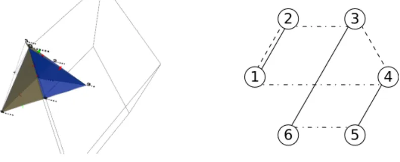
M = M(E, I2) an arbitrary graphic matroid, and B = M(E3, I3) where E3 = {1,2, i, j, k}
(3≤i, j, k ≤n differing) and I3 ={{1},{2},{i},{j},{k},{1,2},{1, j},{1, k},{2, i},{2, k}, {i, j},{i, k},{j, k}}, see Figure 1.
Then the sum A∨M is graphic if and only if B is not a minor ofM with any triplet i, j, k.
1 2
3
4
...
n
1 2
k i j
Figure 1: A graphic representation ofA (left) and B (right) We shall use Tutte’s theorem which is fundamental in matroid theory:
Theorem 2 • A matroid is binary if and only if it does not containU4,2 as a minor.
• A matroid is regular if and only if it does not contain U4,2, F7 and F7∗ as minors.
• A matroid is graphic if and only if it does not contain U4,2, F7, F7∗, M∗(K5) and M∗(K3,3) as minors.
• A matroid is the circuit matroid of a plane graph if and only if it does not containU4,2, F7, F7∗, M∗(K5), M∗(K3,3), M(K5) and M(K3,3) as minors.
Forbidden minors will be of importance in our forthcoming results as well, although they will not appear in our final statement.
2 Results
In most of the cases we speak about graphic matroids so I will call the elements of the matroids edges.
Observe that all but two of the edges of the graph representing the matroidA of Theorem 1 are loops (see Figure 1 as well). Also observe that bridges in a matroid remain bridges of its sum with any other matroid. Hence, in order to generalize Theorem 1 I started to analyze the case when we have only three edges which are neither bridges nor loops. There are two types of matroids with this property, the one with a circuit of length three, and the other with three parallel edges. I found in both cases that there are some forbidden minors so that if any of them appears in the other matroid then the sum is not graphic, while if the matroid doesn’t contain any of them then the sum is graphic.
After these results [7] I started to work with the cases withnparallel edges or with circuits of length n (of course there may be many loops and bridges). After some disappointing results (that thenlong circuit’s cases surely can’t lead to the same type of conditions what I wanted to prove in the other case) the case withn parallel edges lead to a very useful result.
For a transparent presentation of the theorems what will follow, we have to put up some definitions and prove some lemmata, which help us to reduce the infinite number of cases. We study the sum of two graphic matroidsM1 and M2. Throughout we shall refer to M1 andM2 as addends.
It is well known that if a matroid is graphic then so are all of its submatroids and minors.
Hence if a matroid has a non graphic minor then the matroid can’t be graphic.
Definition 3 We call some edges of the matroid serial if they belong to exactly the same circuits.
Definition 4 We call an edge ofM1 essential if it is not a loop in M2 and we call it irrelevant otherwise.
Definition 5 We call a submatroid of an addend devoid if it contains irrelevant edges only.
The following lemmata contain the main opportunities when we want to simplify our addend matroids. It is important that these are valid for graphic matroids only, so I can use graph theoretical concepts.
Lemma 6 Let X and Y denote the set of bridges in M1 and inM2 respectively.
The sumM1∨M2 is graphic if and only if M1\(X∪Y)∨M2\(X∪Y) is graphic.
Lemma 7 If a devoid submatroid X of M1 is a connected component of it then the sum is graphic if and only if (M1\X)∨(M2\X) is graphic.
Lemma 8 M1 is the circuit matroid of a graph G(V, E)in whichX is a connected set of edges andE\X has exactly two common vertices with X (call them aand b).
LetM10 be the circuit matroid ofG0 :=G(V, E∪(a, b)\X) andM20 :=M2\X∪loop(a, b)(Here loop(a, b) denotes a loop corresponding to the edge (a, b) in G0).
If X is devoid then the sumM1∨M2 is graphic if and only if M10 ∨M20 is graphic.
Lemma 9 M1 is the circuit matroid of a graph G(V, E) where X is a connected component of G. If X has only one essential edge x then the sum M1 ∨M2 is graphic if and only if (M1\X∪loop(x))∨(M2\(X\x))is graphic.
The next lemma will be less general, it is only for the cases with parallel edges and loops.
Lemma 10 M1 consist of n parallel edges and k loops. If two essential edgesx andy in M2
are serial then the sumM1∨M2 is graphic if and only if (M1\x)∨M20 is graphic where M20 is defined as follows:
Simply replace the edges x and y in M2 by a single edge xy so that a set S containing xy is independent if and only if S\xy∪ {x, y} was independent. Then xy will play the role of y in M1\x.
After these preliminaries we can define the reduction, what will be the most important concept to reduce the infinite number of cases.
Definition 11 We want to know if the sumM1∨M2 is graphic. We call M2 reduced if none of the lemmata above can help us to decrease the number of edges. (Recall that Lemma 8 can be applied for a special case only while the other four types of simplifications can be applied in any case.)
Corollary 12 M1 andM2 are graphic matroids. Application of the previous lemmata to M2
leads to a reduced matroidM20 whileM1 changes toM10 what we shall call the pair ofM20. Then M1∨M2 is graphic if and only ifM10 ∨M20 is graphic.
We are only one step away from our theorem, but to write it in a pretty way we have to define the following:
Definition 13 Suppose that a matroid has at least three circuitsC1, C2, C3 so that each circuit Ci has at least one element ai satisfying ai∈/ S
j6=i
Cj. (These edges will be called proper edges.) Such a matroid fulfils the three circuits property if at least one of the edges belongs to at least two circuits.
Theorem 14 Let M1 be a matroid which consists of n parallel edges and k loops and let M20 be the matroid reduced from M2. Then M1∨M2 is non graphic if and only if M20 fulfils the three-circuit property.
3 Acknowledgement
The results descussed above are supported by the grant TÁMOP-4.2.2.B-10/1–2010-0009.
References
[1] L. Lovász and A. Recski, On the sum of matroids, Acta Math. Acad. Sci. Hungar., 24, 1973, 329-333.
[2] A. Recski, On the sum of matroids II, Proc. 5th British Combinatorial Conf. Aberdeen, 1975, 515-520.
[3] A. Recski, Matroids – the Engineers’ Revenge, in W J Cook, L Lovasz, J Vygen (eds.) Research trends in combinatorial optimization, Springer, 2008, 387-398.
[4] A. Recski,Matroid Theory and its Applications in Electric Network Theory and in Statics, Springer, Berlin, 1989.
[5] A. Recski, Some open problems of matroid theory, suggested by its applications, Coll.
Math. Soc. J. Bolyai 40, 1982, 311-325.
[6] W.T. Tutte, Introduction to the Theory of Matroids, American Elsevier, New York, 1971.
[7] Cs.Gy. Csehi, Matroidelméleti vizsgálatok és alkalmazásaik, Master’s Thesis, Budapest University of Technology and Economics, 2012.
Strategic interaction games with linear-quadratic payoff
Ahmed Elbanna1, Marianna Bolla1,
1Department of Stochastics, Budapest University of Technology and Economics
Abstract
Strategic interaction is a game in which groups of players are looking for a common goal such as profit, see [1]. The communication between the players is realized through a graph given by its adjacency matrixG, and their strategies also depend on positive parameters δ and α, characterizing the payoffs with and without bilateral influences, respectively.
In the case of strategic complements, and also of substitutes whenδ is ’small’, a unique inner equilibrium exists, and it can be found by matrix inversion and related to the Katz–
Bonacich centrality of the network. However, in the case of strategic substitutes, for larger δ’s (exact limits can be given in terms of the eigenvalues ofGand its complement), corner equilibria appear. To find them, quadratic optimization is used, and in [4] the authors define an algorithm which examines all subsets of vertices for possible corner solutions.
This is computationally not tractable if the number of vertices is ’large’. Instead, we may approximate corner equilibria by spectral clustering tools. More generally, we consider multiple strategies and relate it to the spectrum ofG.
This research was supported by the T ´AMOP-4.2.2.B-10/1-2010-0009 project.
1 Introduction
In many scenarios of strategic interactions, an agent’s benefit of taking a certain action de- pends on the other agents in the same game where players are connected through a graph.
The interaction between agents in a game consisting ofnagents can be described by two main models; games with strategic complements, in which the payoff (benefit) of an agent increases as a result of the actions of the other agents, and games with strategic substitutes, in which the payoff of an agent decreases due to the actions of the other agents. For example when a student buy a book, his friends do not have to buy it anymore because they can borrow it from him for free which is a complementary situation, while a company which expands its market in new country hurts the other companies working in the same field in that country and this is a substitute case. The main goal is to reach the equilibrium state that no player has benefit to change his action taking in consideration the action of the other agents. The set of available actions that each player chooses from, is called strategy and denoted byxi ≥0 (i= 1, . . . , n).
2 Game of strategic complements
Consider a model in which n agents are connected by the simple graph G and acting with continuous strategies: xi ≥0 (i= 1, . . . , n),x= (x1, . . . , xn)T. The payoff of agent iis
ui(x) =αxi−1 2x2i +φ
n
X
j=1
gijxixj,
where α, φ > 0 are given parameters, and G = (gij) is the n×n, symmetric adjacency matrix of G(with 0-1 entries and 0 diagonal). The first two terms are the benefits and costs
of providing the action level xi, while the third term is the effect of agent i’s neighbors as a result of using the actionxi. If this effect is positive as the case in this model (i.e. ∂x∂2ui
i∂xj >0), then the game is called a game of strategic complements and that effect increases the value of agenti’s payoff, but if it is negative as the case in the next section (∂x∂2ui
i∂xj <0), then the game is called a game of strategic substitutes and the third term decreases agenti’s payoff.
For reaching the equilibrium state, the payoff function needs to be maximized for all agents simultaneously, so by using the first order condition:
ui(x)→max (i= 1, . . . , n).
Since
∂ui
∂xi
=α−xi+φ
n
X
j=1
gijxj = 0, i= 1, . . . , n, for the optimalx∗:
x∗i =α+φ
n
X
j=1
gijx∗j, that is,
x∗ =α1+φGx∗. Equivalently,
(I−φG)x∗ =α1, (1)
and
x∗ =α(I−φG)−11.
This is a unique and inner solution (equilibrium) ifI−φGis positive definite, see [1]. There- fore, denoting by λ1 ≥ · · · ≥ λn the eigenvalues of G, 1−φλi >0, and 1−φλmax(G) >0, or equivalently, φ < λ 1
max(G). But λmax(G) ≥ dmin(G), (the minimum vertex degree of G which is ≥ 1), therefore λ 1
max(G) < 1, i.e. φ < 1. Since G is a Frobenius type matrix with zero diagonal, thereforeλ1 =λmax(G) is the maximum absolute value eigenvalue of Gwith eigenvector of nonnegative coordinates,λn=λmin(G)<0 and|λn|< λ1.
In this case, kφGk= φλmax(G) <1 (where k.k denotes the spectral norm), and we can have the following expansion:
(I−φG)−1 =
∞
X
k=0
φkGk =I+φG+φ2G2+. . . Consequently, in view ofα >0,
x∗ =α(
∞
X
k=0
φkGk)1=α(1+φG1+φ2G21+. . .)
where x∗i is α times the so-calledKatz–Bonacich centrality of vertex i; the matrix Gk keeps track of the indirect connections in the network, whilegijk ≥0 measures the number of walks of length k ≥1 in the network from i to j, then P∞
k=0φkgijk counts the number of walks in the network that start at i and end at j and Pn
j=1
P∞
k=0φkgijk is the Bonacich centrality of agentiwith scalar φand it counts the total number of walks in the network that start ati:
x∗i =α[1 +φdi+· · ·+φk(the number of walks of lengthk emanating from i) +. . .] Because of α > 0, this implies that all the coordinates of x∗ are positive (inner solution).
Moreover,x∗i ≥α with equality if and only ifφ= 0.
3 Game of strategic substitutes
Strategic substitutes are less tractable but more realistic and challenging, since its applications include economic competition between firms , people, organizations,...etc, where an agent is hurt by his neighbors’ actions. Consider the payoff function
ui(x) =αxi−1 2x2i −δ
n
X
j=1
gijxixj, (2)
where the first term is the benefit of agentiusing strategy xi, the second is the cost of agent i, while the third term is the effect of agent i’s neighbors as a result of using the actionxi To maximize (2),
∂ui
∂xi
=α−xi−δ
n
X
j=1
gijxj = 0, i= 1, . . . , n (3) For the optimalx∗:
x∗i =α−δ
n
X
j=1
gijx∗j, (4)
if this is positive, otherwise 0. More precisely, x∗i = max{0, α−δ
n
X
j=1
gijx∗j}. (5)
The followings are equivalent formulations of the above maximization task:
1. Find the best strategyx= (x1, . . . , xn),xi∈[0, α] such that xi =
α−δPn
j=1gijxj if δPn
j=1gijxj < α
0 otherwise , i= 1, . . . , n. (6)
2. Consider the best reply function: fi(x, δ,G) = max{0, α−δPn
j=1gijxj}. We are looking for fix points:
xi =fi(x, δ,G), i= 1, . . . , n. (7) By the fix point theorem (Brouwer), since (f1, . . . , fn) : [0, α]n →[0, α]n is continuous, fix point exists and calledNash equilibrium. The equivalence of (6) and (7) is obvious.
3. The quadratic payoff of agenti(2) is to be maximized fori= 1, . . . , nat the same time, subject to xi ≥0 (and xi ≤α), i= 1, . . . , n.
This is equivalent to maximizing the potential function:
P(x, δ) =
n
X
i=1
ui(x) + δ 2
n
X
i=1 n
X
j=1
gijxixj =αxT1−1
2xT(I+δG)x.
It has a unique interior maximum ifP is strictly concave, i.e.,I+δGis positive definite, for which fact a necessary and sufficient condition is that δ < λ −1
min(G). Hence we get the quadratic programming task:
P(x, δ)→max subject to xi≥0, i= 1, . . . , n. (8)
This is equivalent to a linear programming task by the Kuhn–Tucker conditions, see [2].
After differentiatingP with resp. to x, we get
∂P
∂xi =α−xi−δ
n
X
j=1
gijxj = 0, i= 1, . . . , n.
This is the same as (3) subject to 0 ≤ xi ≤ α. Of course, stable equilibrium can be guaranteed only if −(I +δG) < 0, i.e. I +δG > 0, consequently 1 +δλi > 0, ∀i if λi <0, then we get δ < −1λ
i = |λ1
i| ≤ λ 1
min(G).
4. xis a solution of the following system of differential equations:
˙
xi=fi(x, δ,G)−xi, i−1, . . . , n.
xis Nash equilibrium if and only if
˙
x=0. (9)
The equivalence of (9) and (7) is obvious. The Nash equilibrium x is asymptotically stable if and only if xis a locally strict maximum of the potential function φ(this can be treated by Ljapunov functions).
x∗ ≥0 (for all coordinates). In the Nash equilibrium, letA⊂V denote the active agents for whichxi >0 (i∈A), and xi = 0 (i∈A) (such an¯ xis called corner solution). Then xis a Nash equilibrium if and only if
(IA+δGA)xA=α1 and δGA,A¯ xA≥α1
see Proposition 1 of [4]. The explanation is the following: with hypermatrices the above looks like
IA Ø Ø IA¯
+δ
GA GA,A¯
GA,A¯ GA¯
xA
0A¯
=α 1A
1A¯
and (I+δG)x∗ ≥α1.
Using this proposition we can compose a simple algorithm to find all the equilibria for any graph and almost everyδ:
• Given a graphGand δ, consider a subset S⊂V
• Check if det(I+δG)6= 0; if true, proceed; if false, consider next subset.
• Compute xs= (I+δG)−11and set xV−S= 0
• Check ifxi ≥0 andδGV−S,SxS≥α; if true, thenxis an equilibrium, if either condition fails, consider next subset.
• Repeat the procedure for all subsetsS ⊂V.
The down side of this algorithm is that it runs in an exponential time since it checks for each subset of the agents set.Other result from the proposition is how individual equilibrium play relates to graph position. Comparing two agents whose neighbors are nested sets, for δ <1 the agent with the larger set of neighbors plays lower action. Intuitively, an agent who is linked to more outside sources can do less himself. In addition, all equilibria for anyGand almost every δ can be described by the vector of individual Bonancich centralitiesc in GA. For an equilibrium x, simply invert the matrix I+δGA. We then have equilibrium actions xA= (I+δGA)−11 = 1−δc(−δ,GA), and for active player i,xi = 1−δci(−δ,GA). (With negative scalar, an agent’s Bonacich centrality tends to be higher when linked to agents who themselves have few neighbors. The central agents then benefit from their neighbors higher actions and can do less themselves, e.g., freeriders).
3.1 Equilibrium and Bonacich centrality
Here the relation between equilibrium and Bonacich centrality will be shown. For interior equilibrium each player needs the maximum payoff taking in consideration the other agents’
action. By using the first order condition of (2):
α−xi−δ
n
X
j=1
gijxj = 0.
Putting it in the matrix form:
α1−x∗+δGx∗ = 0.
Since Bonacich centrality is in terms of complements, let the decompositionG=C−(C−G), whereCis the adjacency matrix of the complete graph (cij = 1, cii= 0), then we get
α1−x∗−δCx∗+δ(C−G)x∗= 0.
The third term represents the effect of global substitutes, while the forth term represents the effect of the local complements. Adding and removingδx∗:
α1−δUx∗−(1−δ)x∗+δ(C−G)x∗ = 0 whereI+C=U is the matrix of all ones, and sinceUx=x1,x=Pn
j=1xj we get (α−δx∗)1−(1−δ)(I+ δ
1−δ(C−G))x∗= 0, consequently
x∗= α−δx∗
1−δ (I+ δ
1−δ(C−G))−11= α−δx∗ 1−δ y.
where (I+1−δδ (C−G))−1is the Bonacich centrality with scalar1−δδ . To remove the dependance in the right hand side onx∗, we sum up both sides
x∗ = α−δx∗ 1−δ y, wherey=Pn
i=1yi, that leads to
x∗ = αy
1−δ+δyy.
By that we get
x∗ = α−1−δ+δyδαy
1−δ y= α
1−δ+δyy,
where y= (I+1−δδ (C−G))−11. x∗ is a unique interior equilibrium if (I+ 1−δδ (C−G))−1 is well defined and nonnegative, i.e. δ < 1+λ1
max, where λmax is the maximum eigenvalue of (C−G).
Summary:
• Ifδ < 1+λ 1
max(C−G), then a unique inner equilibrium exists (∀xi>0).
• If 1+λ 1
max(C−G) ≤δ < −λ 1
min(G), then a unique equilibrium exits which is a corner or inner point.
• If −λ 1
min(G) ≤δ < 1 then there are multiple equilibria among those there are corners.
In this case, only corner equilibria can be stable.
Explanation: an interior equilibrium can only be at a saddle point, since the Hessian is not negative definite and the function to be maximized is a non-concave quadratic function.
Then, there must be a direction along which the potential increases without bound. Hence, the vector must not be interior, and maximum is taken on at the boundary (see Proposition 3 of [4]).
Ifδ= 1 (see [3], the stable equilibrium is corner: xA=1, whereAis a maximal independent set of V. There can be many maximal independent sets in a graph (for example, there are k such in case of the complete k-partite graph; especially, 2 in the star, which is a complete 2-partite graph), hence there can be finitely many stable equilibria. To approximate corner equilibria, we plan to use spectral clustering methods which work in polynomial time (see [5]).
References
[1] C. Ballester, A. Calvo-Armengol, Y. Zenou, Who’s who in networks. Wanted: the key player,Econometrica74 (5), 1403-1417.
[2] M. S. Bazaraa and C. M. Shetty, Nonlinear Programming, Theory and Algorithms.
Wiley, 1979.
[3] Y. Bramoull´e, R. E. Kranton, Public goods in networks, Journal of Economic Theory 135(2007), 478-494.
[4] Y. Bramoull´e, R. E. Kranton, M. D’Amours, Strategic interaction and networks (2012), unpublished manuscript, Duke University.
[5] M. E. J. Newman, Finding community structure in networks using the eigenvectors of matrices, Physical Review E 74, 036104 (2006).
Projections of Mandelbrot percolation in higher dimensions and Evolutionary Apollonian Networks
Lajos Vágó1, Károly Simon1,
1Department of Stochastics, Budapest University of Technology and Economics
My research may be divided into two main parts. From the one hand, we generalized the results of Rams and Simon obtained for the non-emptiness of the interior of projections of Mandelbrot percolation to the higher dimensional case. On the other hand, network models Evolutionary Apollonian Networks introduced by Zhang, Rong and Zhou was studied.
1 Projections of Mandelbrot percolation
1.1 Most important notations
We denote by E=E(ω)thed-dimensional Mandelbrot percolation on the unit cube K, with retaining probabilitiespi(1),...,i(d),i(j)= 1, . . . , M. Fix 1≤k≤d−1. Forα= a(1), . . . ,a(k)
, a(1), . . . ,a(k) orthogonal unit vectors inRd letPα be the plane spanned by the vectors in α:
Pα =span{a(1), . . . ,a(k)}.
We consider the orthogonal projections Πα ofE to each k-dimensional planes Pα. Note that this projection is the higher dimensional pair of projectionprojαof [2]. Our goal is to determine the parameters pi(1),...,i(d) for which almost surely int{ΠαE} 6=∅ for allα, conditioned on E being nonempty.
In addition, we consider radial projections as well, i.e. given t∈Rd, the radial projection with centertof setE is denoted byP rojt(E) and is defined as the set of vectors under which points ofE\ {t}are visible from t.
It will be useful to handle projections parallel to some sides of the unite cube separately from other directions.
Assumption 1.1. Let us first consider only the nonparallel planes, i.e. for which there exists a vector v∈P⊥α such that vi 6=0 for all i= 1, . . . , d.
1.2 Results
Later we will define Condition A(α) on the set of probabilities pi(1),...,i(d), i(j) = 1, . . . , M, which is the most important tool for the following theorems. At this point it is enough to know that ifpi(1),...,i(d) > M−(d−k) for alli(j)= 1, . . . , M, then ConditionA(α)holds for allα.
Theorem 1.2. Let d and 1≤k < d be fixed, and suppose that Condition A(α) holds for all α satisfying Assumption 1.1. In addition, to control parallel directions we suppose that for all distinct j1, . . . , jk∈ {1, . . . , d} and for alli(j1), . . . , i(jk)∈ {0, . . . , M −1}
M−1
X
i(jk+1),...,i(jd)=0
pi(1),...,i(d) >1,
where {jk+1, . . . , jd}={1, . . . , d} \ {j1, . . . , jk}. Then almost surely for all α orthogonal pro- jectionsΠα(E) have nonempty interior, conditioned on E being nonempty.