PHYSICSBUDAPEST INSTITUTE FOR RESEARCH CENTRAL V- h3$

KFKI-70-15 NAC

G . Németh B. G ellai

G . Jancsó APPLICATION O F THE MINIMAX APPROXIMATION T O THE REDUCED PARTITION FUNCTION O F

ISO TO PIC MOLECULES

S%an^axian Sftcademy^ of (Sciences

CENTRAL RESEARCH

INSTITUTE FOR PHYSICS

BUDAPEST

2017

Printed in the Central Research Institute for Physics, Budapest, Hungary

Kiadja a KFKI Könyvtár Kiadói Osztály O . v . : Dr.Farkas Istvánná

Szakmai lektor: Molnár József Nyelvi lektor: Kovács Jenőné

Példányszám: 187 Munkaszám: 5067 Készült a KFKI házi sokszorosítójában Felelős vezető: Gyenes Imre

G. Németh, В. Gellai, G. Jancsó

Centrál Research Institute for Physics, Budapest

1. Introduction

The reduced partition function ratio of isotopic molecules introduced by Bigeleisen and Mayer [l] in the statistical mechanics of isotopic systems has the form

3N-6

П

i=l -u

e T--

i /2 1 1

/1^.1^/

where u^ = hcun/kT, is the i-th normal vibrational frequency /in cm *7, 3N-6 is the number of internal degrees of freedom for a molecule with N atoms /3N-5 for a linear molecule/, while u' and u^ stand for light and heavy isotopic species, respectively.

The logarithm of the reduced partition function ratio

where

ln s/s'f = l £ln b(u') - In b(ui)J /1 .2 /

In b(u) = -In u + u /2 + ln(l - e- u ) /1.3/

can be expanded into appropriate power series which permit the quick numerical evaluation or the estimation of the equilibrium constants of isotopic exchange

2

reactions, the isotope effect on rate constants and the thermodynamic quantities of the isotopic systems. The approximation to In s/s'f in terms of an even power series helped in the understanding of the nature of isotope effects.

The reduced partition function ratio and the isotope effect on the thermodynamic properties can be evaluated without actually solving the

secular equation by using the method of moments [2,3] and an expansion in the even powers of u^ [2,4,5]. Bigeleisen and his coworkers used Chebyshev and Jacobi polynomials [4,5], which are interpolating polynomials, and yield a better approximation than the Bernoulli series [2] based on the Taylor

expansion, while the covergence is not subject to the restriction u' < 2x.

\ m ax

In the present work the different methods used for the expansion of Eq. /1.2/ are briefly reviewed and then a method which gives the best /mini­

max [б]/ approximation to In b(u) will be described. The error curve of this approximation has as many extrema as possible at any given order of t-he expansion and the maxima and minima of the error curve have the smallest possible values. This high frequency and small amplitude oscillation of the absolute

error is precisely the feature needed for a good approximation to In s/s'f.

2. The polynomial expansions of s/s'f or In s/s'f

Usually it is not the reduced partition function ratio s/s'f itself, but its logarithm In s/s'f which is expanded into a power series [7].

Let us see first the expansions methods which permit the quick numerical evaluation or estimation of In s/s'f.

The expansion developed and used by Urey for the evaluation of the equilibrium constants of a number of isotopic exchange reactions [в] reads as

In s/s'f=£ln

i

I К

12 6 i coth x.^ (coth2x^ - l) + . . .^j /2.1/ where

+ u,

/2.2/

This expansion converge rapidly /see Appendix I/ and can be used in most 3

cases without the term in 6^. A similar expansion was formulated by Waldmann already in 1943 [9].

For the numerical evaluation of In s/s'f the most succesful seems to be the G(u) expansion introduced by Bigeleisen and Mayer [l] . The result of the expansion which to first order has the form

In s/s'f = £ G (u i) /2.3/

was extended to third order [2j as

In s/s'f

С(и±) - 23(4^)

/2.4/

where

G(u± ) /2.5/

and

/2.6/

/2.7/

The functions G (u^), s(u^) and с(и^) have been tabulated for different values of u^ [10,1]. The convergence restriction on this series is that Au^/u^ < 1 , thus it converges for all the physically possible values of u^

and Au^ /see Appendix II/. The G(u") expansion was extended by Vojta to order n [7,11] as

ln s/s'f = I I ( -l)k Gk (u )(Au )}

i k=l

/2.8/

G l K )

1 _1_

2 u ,

e - 1

-G(u i) /2.9/

Gk<uP - A - FT Í "

ku n-1

k-i ~nui e

>

к = 2 /2.1 0/

4

An approximation in the form

-hc(o£/2kT e_________________r —

-hcw^/2kT e

-hco)i /кТ \ / _

-hcu)| /кт'у w ni I ^/2.11/

was introduced by Tatevskii [12,13]. This approximation works well at higher temperatures and the equilibrium constant of an isotopic exchange reaction can be evaluated in a simple manner from the ratios of the symmetry numbers of the participating isotopic molecules. If the zero point energy cannot be ignored

the author used instead of Eq. /2.11/ the expression

-hcw|/2kT / -hcu)^/kT e______ V 1 - e____ '

-hcw^/2kT / -hccoj /кТ e ( 1 - e

The function y^ has been evaluated and tabulated for various values of

«i/»i and <Dj/Т. Since the exact meaning of the function y^ is not clear and the expressions are fairly complicated, the Bigeleisen-Mayer G(u) approximation is preferably used for the calculations.

At lower temperatures the isotopic difference in the zero point energies plays an important role. The zero point energy difference was approximated by Bigeleisen and Goldstein []l4j in terms of a Taylor series o) even powers of the frequencies around an arbitrarily chosen point A as

T ^/2.12/

о iI O í " w i)

l

i 6 A ,

( - 1)P+1 ( 2p - 2)i i p =2 22p 1 (p-l)l

/2.13/

Py1 ( - Q 3 6Xi~J

jio AP-j

J о

where

>. = 4n2c 2 /2.14/

J. I

ЛА^ = >{П - /2.15/

The value of A must be selected from the frequency spectrum by considering that the condition of the convergence is that

/2.16/

This expression was used for studying the relations between the zero point energies of isotopic homologues [l5] .

In the formulation of the relationships between the reduced partition function ratios of multiple isotope substituted molecules the Bernoulli series

[

]

In s/s'f = l l C - l ) ^ 1 ~ 2i o 'TVf. 6Cu i^) /2.17/

i j=l J v J >

where B 2j-i are the Bernoulli numbers [l6] , б(и2^) = u ^ 2^ - u 2^ , proved to be useful. Because of the convergence restriction u ^ ax < 2тг on the Bernoulli series, this expansion can be applied only at higher temperatures and to molecules with not too high frequencies. Vojta [17] has given two new proofs of the Bernoulli series expansion. The first term in Eq./2.17/ is the first quantum correction to the reduced partition function ratio of isotopic molecules from which a fundamental expression for the description of the isotope effects of equilibrium systems can be obtained [2] as

£ ( й У I N ' 1 - ' 2 - w

rfhere m^ is the mass of the i-th atom in the light, пк that in the heavy isotopic molecule and a ^ is the Cartesian force constant of the i-th atom in the molecule.

In the у method [2] proposed for extending the validity of the Bernoulli expansion is defined as

Yj^ = 12G(u^)/u^ /2.19/

which, introduced into Eq./2.3/ yields

u.

ln s/s'f = I i2 Ä u i /2 .20/

Since y^ does not decrease very rapidly with u^, an average value у can be defined if the frequencies of the molecule lie within a narrow range and we can write

6

ln s/s'f = J 6uJ . /2.21/

The applicability of Eq. /2.21/ has been investigated by several authors [18,19,20,21,22].

The restriction u' < 2v to the convergence of the Bernoulli max

series was removed by Bigeleisen and Ishida [4] who vised shifted Chebyshev polynomials of the first kind for the expansion into even powers of u| and u^. They started from the expression of In b(u)[23] as

°° Г

,

In b(u) = ] In 1 + • /2.22/

This infinite series converges for all values of u. Applying the т method proposed by Lanczos [24] Bigeleisen and Ishida obtained

n (-l')m+1 В u2m

In b ( u ) - --- 2m(> y T (n '1" ' V1x) '2-23'

where

Tfn,m,u ^ =

^ 9 ' max s

1

/ Í

p=m J p=o

R - ( “» a x ' 2’)2 and

c n = С-1)П+Р 22p n(n+p - l)l/(n-p)l (2p)!

Then

In s/s'f

( -

)

6u2m

Tfn,m,u ]

\ ' ' m a x /

/2.24/

/2.25/

/2.26/

/2.27/

The expansion /2.27/ differs from the Bernoulli series /2.17/ essentially only by that each term is multiplied by the modulating coefficient

T(n,m,umax] and this causes the new series to converge much faster than the Bernoulli series.

The method was extended to the group of the Jacobi polynomials [5]

p ( V ^ )

n ^{( X}) 1 + n m=l

I

xm

m -1 (-п+к)(п+у+6- 1+к)

(Y+k)(1+k) /2.28/

The expansion of the logarithmic terms in Eq. /2.22/ applying the т method and usinq a common range R = (u ' /2ttV , with u' being the hiqhest

frequency of the light isotopic molecule, leads to the expression

In s / s 'f = n m=l

l

( -

)

2m (2m)!

2m

т 1,'5(п '” 'им х ) " /2-29/

The approximation to In b(u) could be improved by subdividing the range of the expansion variable. On dividing the summation of Eq. /2.22/ into two parts they obtained

L In b(u) = \ In

k=l

00

+ У In k=L+l

/2.30/

where L is a finite, positive integer. It was shown that the approximation to In b(u) improves with increasing values of L, but the use of higher values than 5 does not seem to be worth while.

A search was made Q>] for the "best" Jacobi polynomial by minink -' - the weighted root-mean-square-error /RMSE/ expressed as

RMSE

mav

j w(u) [e (u) - ё] 2 du max

$

/2.31/

where w(u) is the weighting function and e is the mean of the absolute errors of the expansion of In b(u) expressed as

umax

w (u-) e(u) du

£ =

max

w ( u ) du

/2.32/

8

With the assumption of w(u) <* u the RMSE was numerically evaluated for the systematically varied two parameters у and 6 of the Jacoby polynomial.

By comparing the results the "best" Jacobi polynomial was obtained for every combination of the fixed range um=v = Itt, 2tt,...,8tt, and order n = 1,2,3,4

m a x

for both L = 0 and L = 5. The parameters у and 6 of the "best" Jacobi polynomials were listed in tabulated form. Since the weighting function w ( u ) depends on the frequency distribution in the molecule and on the values of the isotopic shifts on the frequencies in order to find the "best" Jacobi polynomial for a given molecule it might be necessary to establish a suitable weighting function in each case.

In the method to be described in the following for the approximation to In b(u) polynomials in terms of the even powers of u^ are used, the convergence restriction u' < 2tt on the Bernoulli series is removed and

max

the amplitude of the error curve is as small as possible.

3. The mlnimax approximation to In b(u)

definitions and theorems which will be briefly recalled before showing its use for the function In b(u ) . The aim is to expand the function In b(u) into a series of even powers of u. Let H be a set of the polynomials

p n (ui = l ak u 2k /3.1/

k=o

and Q n (u) 6 H be the polynomial for which the expression

The so-called minimax approximation method [б] is based on some

max 0<u<u

I In b(u) - Pn (u ) I /3.2/

max

hcto

has a minimum value /u = --- , ™ ax— /. The polynomial Q (u ) is the

ГПЭ. X К i n

minimax approximation to the function In b(u). Using the notation

En = max I In b(u) - Qn (u)| 0 < u < u

max /3.3/

the error function obtained by the Qn (u) polynomial in the form

E ^ u 4) = In b ( u ) - Qn(u) /3.4/

takes by the Chebyshev theorem [25j its extreme values -E at n+2 distinct points, with alternating sign in the interval [o,u x] , that is

En (u^) = cxE^ , — -ctEn , E n (u^ ) — uE^ , ... /3.5/

0 i ui < u 2 < u 3 ... £ umax ; a = ± 1

Conversely, if there is a polynomial which approximates the function with a deviation having its extreme values at n+2 distinct points, with alternating sign in the interval of the approximation, then this polynomial is the minimax approximation of the function in question. Unfortunately, no explicit formula can be given for the coefficients of the minimax approximation to a function, but there are some numerical processes by which they can be evaluated to a desired accuracy. By using these methods the error function of some initial approximations to a given functions can be improved so that it obtains the properties characterizing the error function of the minimax approximation. The partial sum of the Taylor expansion, some interpolating polynomials, the partial sum of some orthogonal expansions, the expansion formula fór In b(u) obtained by Bigeleisen and Ishida with the use of the Lanczos т method [4] etc. can be regarded as initial approximation.

To formulate the minimax approximation to In b(u), it is first expanded in terms of Chebyshev polynomials, second the Chebyshev coefficients are improved by the method of Hornecker [2б] and finally a numerical test is performed to see whether the error function has the properties required by the Chebyshev theorem.

The Chebyshev expansion of the In b (u) is written in the form

c 00

In b(u) = — ■ + I ck T*(x2 ) О < x < 1 /3.6/

к— 1 where

x = u О < u < u

max max /3.7/

i

= I \ ln b (X -Umax) Tk 0 2) — Т - Ц Т dx

r\ V J. X

/3.8/

and

ть(х2) = cos [k arc cos (2x 2 - l)] k=0 ,l,2 ,... /3 .9 /

IO

Stands for the orthogonal polynomials transformed to [ o ,l]interval, the so- called Chebyshev polynomials [24]. Unfortunately, the integrals /3.8/ can be evaluated only by numerical processes.

For the calculation of the coefficients c^ , use is made of the expansion of In b(u) given by Eq. /2.22/ and the equation

1

In (1+x) - x j * /3.10/

о Eq. /2.22/ can be thus rewritten as

ln b(u') = I u 2 2 ~ 7 T k=l 4it к

1 -

° 1 + 7 T T 2 У 4 TT к

dy • /3.11/

Using an even power series expansion of the function 1

A1 + ^)l 2 7 j

=

I

1 + ^{u m=o}

7 7

and substituting it in Eq. /3.11/ we obtained the polynomial approximation to In b(u) as

2 n ln b(u ) = y j I b.

m=o

C(2m +2) 1 m £(2 ) m + 1

2m . „

u + H /3.13/

where

/3.14/

and 5(m) = £ l/£m the Riemann zeta function. For the estimation of the

£=1

error H of In b(u) we get by /3.14/

|H| < — SJ2- |h| /3.15/

On multiplying the coefficients bm of the approximation /3.12/ by r^2^(mil) an<^ Ь У rearran9 in9 this polynomial approximation in terms of

Chebyshev polynomials [24] we get the approximate values of the coefficients c^ defined by Eq. /3.8/. On improving the approximate values of the coeffici­

ents c^ by the Hornecker method [26] we get the coefficients of the mini­

max approximation of the function In b(u).

The curves for the absolute error in In b(u) obtained by the mini­

max approximation over the ranges [o,4ir] and [o,8ir] as a function of u for orders n = 1-4 can be seen in Figs. 1 and 2, respectively. For comparison also the error curves plotted for the Chebyshev /L=0, L = 5 /, and the "best"

Jacobi polynomial approximations of Bigeleisen et.al. [5] are shown. It is apparent from the figures that the shape of the error function for In Ь(и) has the properties of the minimax approximation: it exhibits uniform small amplitude oscillations on both sides of the abscissa and has the number of extrema required by the Chebyshev theorem.

Fig. 1

Intercomparison of the absolute error in In b(u) obtained by various V

approximations over the range [o,4tt] as a function of u for orders n = 1-4

... "Best" Jacobi polynomial L=5, --- Chebyshev p oly­

nomial L=5, Chebyshev polynomial L=0 [5], __________

minimax approximation.

1 2

Intercomparison of the absolute error in ln(u) obtained by various approximations over the range [0,8if) as a function of u for orders n = 1-4

... "Best" Jacobi polynomial L=5, --- Chebyshev p o l y ­ nomial L=5, Chebyshev polynomial L=0 [5], _________

minimax approximation.

The 1th derivative of the expression /2.22/ can be written as

In b(u) = (-I)* (f-l)l

k=l ^4tt^

/3.16/

It can be shown that the derivative of any order of the function In b(u) is nonzero over the range

C0 'umaxl

common u^ ax determined by the highest frequency of the light isotopic molecule.

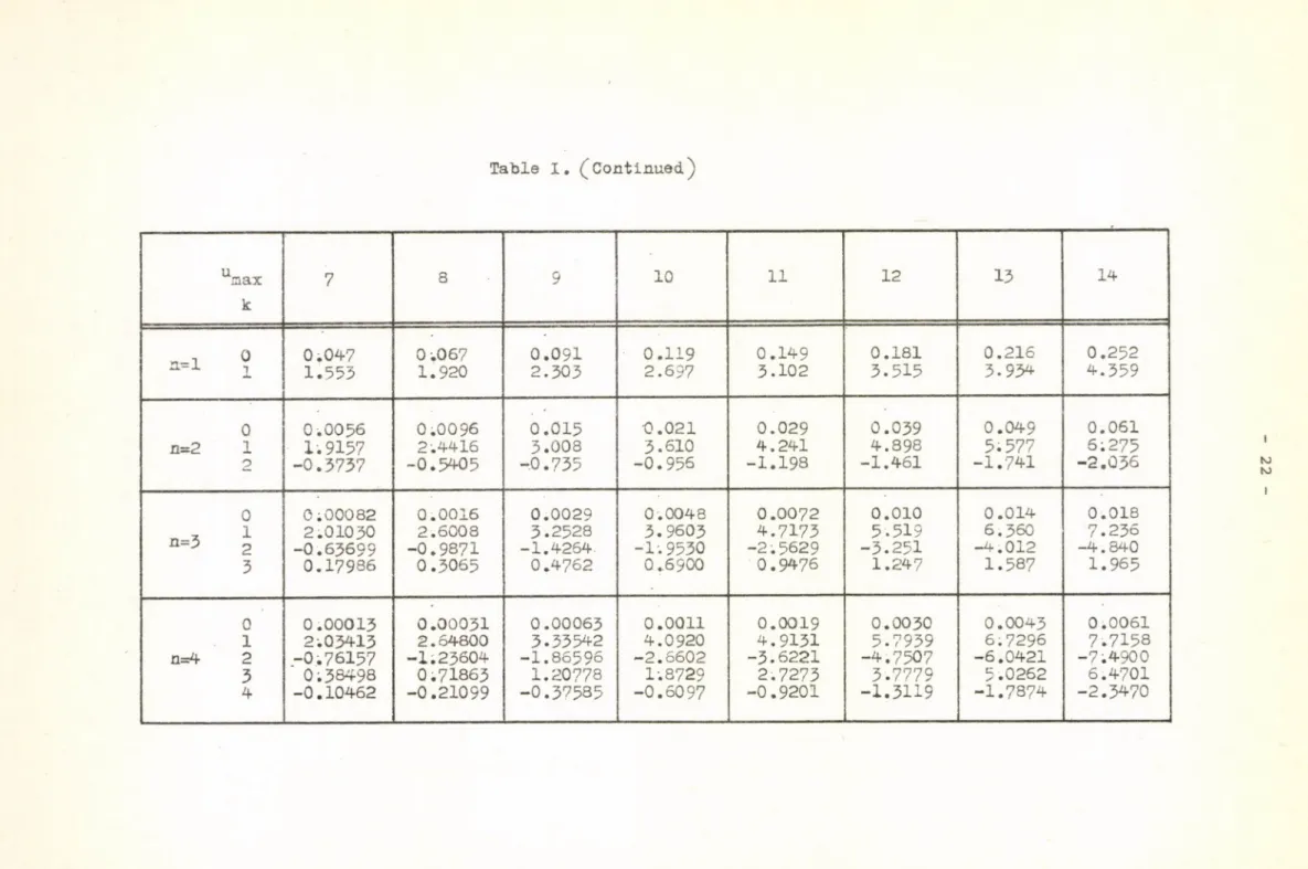
The coefficients a (n A i u,na x ) of the approximation

in b ( u ) = I a(n,k,um a x ) . (u/um a x )2k /3.17/

for u = 1,2,...,30 and for n = 1-4 are listed in Table I. /As mention- mőix

ed above, the coefficient a(n,0 ,u x ) of the approximation equals the amplitude of the error curve./

The coefficients a (n 'k 'um a x ^ as a function of n and к are shown in Figures 3,4,5, while the absolute error as a function of n for u = 2 0 and 30 can be seen in Fig. 6 .

max 3

Fig. 3

Coefficients of the minimax approximation to In b(u) as a function of u for n = 1 ,2 .

max '

J.

Fig.

Coefficients of the minimax approximation to In b(u") as a function

o f u

m a x for n = 3.

a(n.k,UnJ

Fig. 5

Coefficients of the minimax approximation to In b(u) as a function

of umax for n = 4 *

Fig. 6

Absolute error in In b(u) obtained by the minimax approximation as a function of n, the order of the expansion for u = 20, 30.

The variation of the absolute error with u__„ for different values of nITlaX is plotted in Fig. 7.

It can be shown that the error of the (n+1) — th order approximatioi becomes for large orders equal to the error of the n-th order approximation multiplied by q, Since

lim n-*-°°

Jn+1 /3.18/

/see Appendix III/. For large values of umax » 4 is close to unity. This means th\,at the error decreases very slowly w ith increasing n, e.g. for u = 2 0 and u = 30, q = 0.54 and q = 0.66, respectively. Thus, the error is not reduced even by half if the order of the approximation is

increased by one. Consequently for too large umax a few terms cannot give a good convergence.

JLO

Fig. 7

Absolute error in In b(u) obtained by the minimax approximation as a function of u„ and n, the order of expansion.

max ^

The absolute values of the percent error of the approximation over the range [0,20] as a function of n = 2,4,6 are shown in F i g . 8.

On substituting Eg. /3.17/ into the expression /1.2/ we obtain

in als'f.

3T

where

Fig. 8

Percent error in in b(u) obtained by the minimax approximation over the range [0,6tt] as a function of u and n, the order of

expansion.

6 / u'

max u,2k

max

/3.20/

“ max can ke est;*-mated without actually solving the secular equation by applying the "row-sum and column-sum" method used by Bigeleisen et.al. [5].

In the next chapter some applications to polyatomic molecules, an analysis of the accuracy obtainable and a comparison of the results of the minimax approximation with those obtained by Bigeleisen et.al. [5] will be presented.

4. Application of the minimax method У

The minimax approximation method was used for the evaluation of the reduced partition function ratios of some pairs of isotopic molecules and the approximations to the exact values were compared with those obtained by other methods. For the exact calculations of In s/s'f the individual molecular frequencies were evaluated by using the Wilson FG-matrix method [29] . The

18

value of u' was computed at each temperature from the highest molecular IHclX

frequency of the system and rounded off to the next higher integer. The

coefficients of the plynomial for the rounded value of u^,ax were taken from Table 1. The temperature range covered by the calculation was chosen to be wider than that which is experimentally significant.

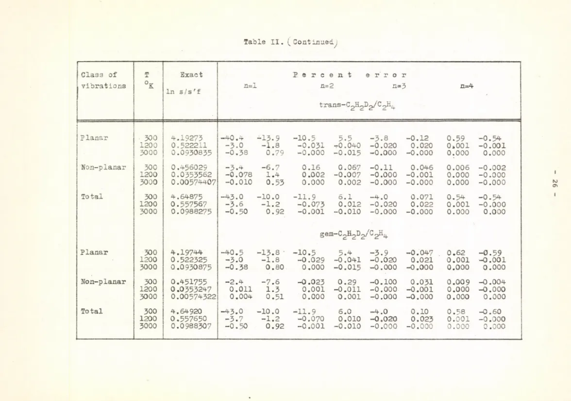
In Tables II-IV the intercomparison of the Chebyshev expansion [4], the "best" Jacobi polynomials [5] and the minimax approximation with the exact values of In s/s'f for isotopic pairs in ethylene and methane is presented. /The coefficients of the Chebyshev polynomials were evaluated by using the "running u" method [4]./

For the deuterated ethylene molecules /Table II/ the value of In s/s'f of every isotopic pair was evaluated separately for the planar, non-planar and total vibrations of the molecule. It can be seen that the errors for the non-planar vibrations are smaller than those for the planar and total vibrational spectrum. This is due to the smaller value of u' x which determines in the first place the error of the minimax approximation,

/

and to the narrower range of the non-planar vibrations. It can be seen that in the case of the total and planar vibrations the minimax method gives bfetter results than the Chebyshev expansion, especially so, at room temperature and low values of the order n. The accuracy of the minimax approximation is not worsened if more protium are substituted by deuterium.

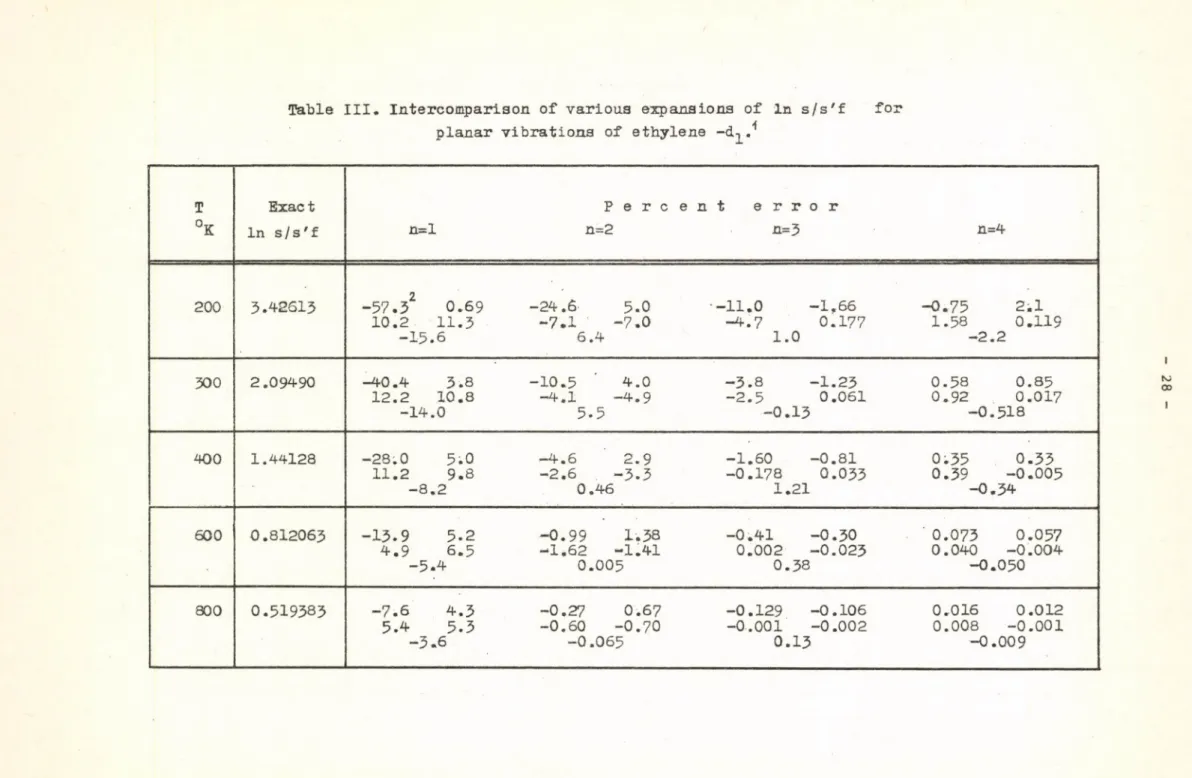
The intercomparison of the different approximations to the In s/s'f for the planar vibrations of mono-deuteroethylene /Table III/ is difficult because of the fact that different Chebyshev /L=0, L=5/ and "best" Jacobi

/L=0, L=5/ polynomials yield the best results at different temperatures and orders, i.e. the "best" Jacobi polynomials are not always the best. A detailed inspection of the values in Table III, however, shows that the minimax method gives in this particular example at least as good results as the other

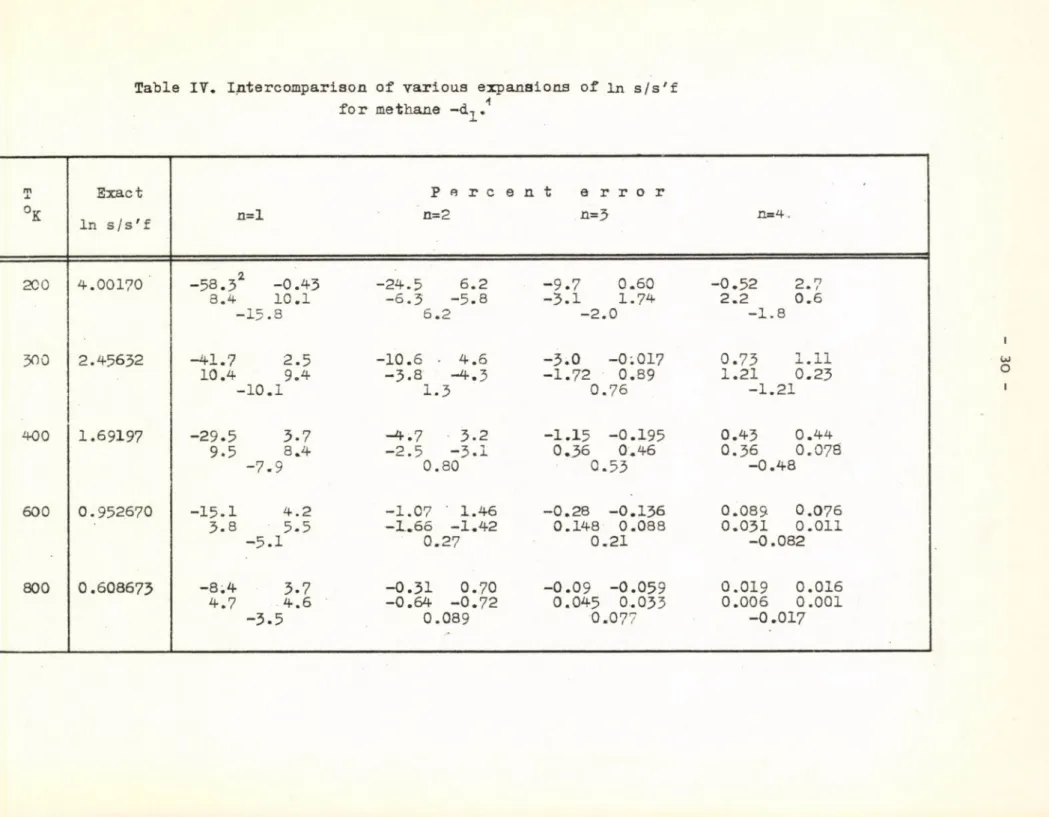
approximations. Similar conclusions can be made from Table IV for the mono- deuteromethane.

The results of the minimax approximation in the case of the deuterated methyl halide molecules /Table V / show that at lower temperatures even for high values of In s/s'f the method works very well. The maximum error, 11.1%

is obtained in the case of CD^F-CH^F at 200°K and n=l.

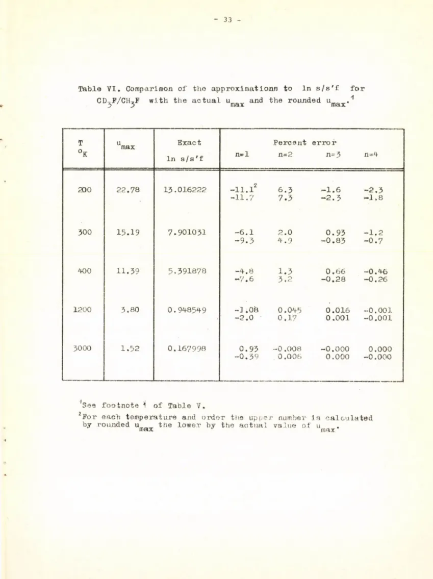
In table VI the results obtained by using the actual value of u '

J 3 max

are compared with those obtained by using the rounded off value for the Vi

evaluation of the coefficients of the minimax approximation in the case of CD,F-CH,F. If one uses the actual values of u ' the occasional breaks in the monotonous trend of the approximation disappear but it may worsen to some extent. Consequently, it presents no special advantage to use the actual value

of u ^ , not to mention the difficulty caused by the necessity of evaluating the minimax approximation coefficients of In b(u) every time the actual value of u' is used. .

max

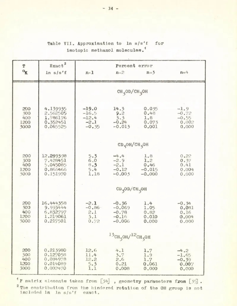
The results for isotopic methanols, summarized in Table VII show

13 12

for the C H 3OH- CH-jOH pair of isotopic molecules the iresults are not better but in some cases even worse than those obtained for the deuterated methanol molecules. This is not surprising if one considers that the error of the approximation is determined above all by the value of uj^ax which is the same for all the isotopic methanol molecules.

It can be seen from the intercomparison of the approximations in the case of deuterated water molecules /Table VIII / that about room temperature the Bigeleisen-Mayer G(u) expansion gives the best, while the minimax method the second best results. The Bernoulli expansion cannot be applied at room temperatures at which the condition u^ ax < 2тг does not hold. At temperatures of 1200°K and 3000°K the Chebyshev and the minimax approximations yield similar results and both are better than those obtained from the Bernoulli series. It is of interest to note that the percent errors are about equal for the HDO-I^O and D2O-H2O pairs of isotopic molecules although the value of In s/s'f has doubled by the introduction of the second deuterium into the H^O. It is apparent from Fig. 9 in which the errors of the minimax approximation for the different vibrations of the K^O, HDO, D 2O molecules are shown, if one uses a polynomial corresponding to umax ~ 19 and n=l, that the increase in the percent error on replacing protium by deuterium in HDO is due primarily to the shift in the tdj vibrational frequency.

As a general rule it is found that the accuracy of the approximation is sensitive to the distribution of the frequencies of a given pair of isotopic molecules. Therefore it can be hardly predicted how many terms of the polynomial are needed to obtain a given accuracy. An analysis of the calculated examples shows that at about room temperature /300°K/ the maximum error of the approxi­

mation is not more than 20% for n=l, 10% for n=2 and vl% for n=3. In a favourable case the error of the approximation may be much smaller.

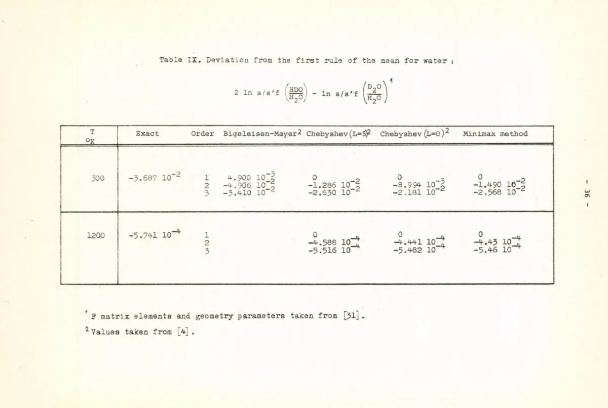
The relationship between the "rules of the mean" and the polynomial expansion of In s/s'f is thoroughly discussed by Bigeleisen and Ishida [4].

Considering the minimax approximation from this point of view,, we find that e.g. in the case of deuterated water molecules /using w' of H_0 for the evaluation of the coefficients of the polynomial for both isotopic pairs/

the minimax approximation predicts zero quantum correction to the first order, thus satisying the first rule of the mean, /Table IX /. In order to approximate the exact value of the quantum correction it is necessary to use a polynomial with at least n=3.

20

Error curve for the minimax approximation to In b(u) for isotopic water molecules /u = 19, n = 1/.

umax к

1 2 3 4 5 6

0 0 . 0 0 0 0 4 2 0 .0 0 0 6 3 0 : 0 0 2 9 0 .0 0 8 0 0 : 0 1 7 0 . 0 3 0

1 0 .0 4 1 3 2 5 0 .1 6 1 4 4 0 . 3 5 0 3 0 . 5 9 5 2 0 . 8 8 4 1 . 2 0 6

0 0 .0 0 0 0 0 0 1 6 0 .0 0 0 0 0 9 5 0 . 0 0 0 0 9 2 0 . 0 0 0 4 2 0.0013 0 . 0 0 2 9

a = 2 1 0 .0 4 1 6 6 3 6 6 0 .1 6 6 4 9 0 7 О.373254 0 .6 5 8 4 2 1 .0 1 5 9 1 .4 3 7 8

2 - 0 . 0 0 0 3 3 9 1 4 - 0.0050704 - 0 . 0 2 3 1 1 9 - 0 . 0 6 4 0 4 - 0 . 1 3 4 6 - 0 . 2 3 7 8

0 0. 0 00 0 0 00 1 0 .0 0 0 0 0 0 1 7 0 .0 0 0 0 0 3 5 0 .0 0 0 0 2 6 0 . 00 0 1 1 О.ООО34

П - Л 1 0 .0 4 1 6 6 6 6 4 0 .1 6 6 6 6 1 1 1 0 .3 7 4 8 8 4 6 0 .6 6 5 7 6 5 1 .0 3 7 6 5 1 .4 8 7 3 7

** J 2 - o.00034710 _- 0.00553713 - 0 . 0 2 7 5 1 2 4 - 0 . 0 3 3 9 7 2 - 0 . 1 9 4 1 6 - 0 . 3 7 4 6 7

3 0 .0 0 0 0 0 5 3 1 0.00030533 0 .0 0 2 9 4 7 3 O .O I3427 0 .0 4 0 3 1 0 .0 9 3 0 6

0 0 .0 0 0 0 0 0 0 0 0 . 0 00 00 0 0 0

V

0 .0 0 0 0 0 0 1 4 0 .0 0 0 0 0 1 8 0 . 00 0 0 11 0 .0 0 0 0 4 4

1 0 .0 4 1 6 6 6 6 7 0 .1 6 6 6 6 6 5 0 0 .3 7 4 9 9 2 6 2 0 . 6 6 6 5 7 2 6 1 .0 4 1 0 6 7 1 .4 9 7 5 3 5 n=4 2 -0:00034722 - 0 . 0 0 5 5 5 4 2 0 - 0 . 0 2 8 0 6 3 5 1 - 0 . 0 8 8 0 8 2 8 - O .2I I 7O5 - 0 . 4 2 7 3 3 8

3 O.OOOOO55I 0 .0 0 0 3 4 8 8 4 0 .0 0 3 8 4 5 5 0 0 .0 2 0 0 8 3 8 0 .0 6 8 8 7 6 0 .1 7 9 2 3 6

4 - 0 . 0 0 0 0 0 0 1 0 -O.OOOO2I7B - 0 . 0 0 0 4 4 6 3 6 - 0 . 0 0 3 3 5 6 9 - 0 . 0 1 4 4 5 8 . - 0 . 0 4 3 8 1 2

Table I. (Continued.)

uaax к

7 8 9 10 11 12 13 14

n 1 0 0.047 0.067 0.091 0.119 0.149 0.181 0.216 0.252

n-1 1.553 1.920 2.303 2.697 3.102 3.515 3.934 4.359

0 0.0056 0.0096 0.015 0.021 0.029 0.039 0.049 0.061

n=2 1 1.9157 2.4416 3.008 3.610 4.241 4.898 5.577 6:275

2 -0.3737 -0.5405 -0.735 -0.956 -1.198 -1.461 -1.741 -2.036

0 0;00082 0.0016 0.0029 0.0048 0.0072 0.010 0.014 0.018

-x 1 2.01030 2.6008 3.2528 3.9603 4.7173 5.519 6.360 7.236

n-3 2

-0.63699 -0.9871 -1.4264 -1.9530 -2.5629 -3.251 -4.012 -4.840

3 0.17986 0.3065 0.4762 0.6900 0.9476 1.247 1.587 1.965

0 0.00013 0.00031 0.00063 0.0011 0.0019 0.0030 0.0043 0.0061

1 2.03413 2.64800 3.33542 4.0920 4.9131 5.7939 6.7296 7.7158

n=4 2 -0.76157 -1.23604 -1.86596 -2.6602 -3.6221 -4.7507 -6.0421 -7.4900

3 0.38498 0.71863 1.20778 1:8729 2.7273 3.7779 5.0262 6.4701

4 -0.10462 -0.21099 -0.37585 -0.6097 -0.9201 -1.3119 -1.7874 -2.3470

umax к

15 16 17 18 19 20 21 22

n=l x 0.290 4.790

0.330 5.224

0.371 5.662

0.414 6.104

0.457 6.548

0.502 6.994

0.548 7.443

О. 5 9 5

7.894

0 n=2 1 2

0.074 6.990 -2.345

0.088 7.719 -2.666

0.103 8.461 -2.998

0.119 9.215 -3.340

0.136 9.978 -3.690

0.153 10:751 -4.048

0.172 11.531 -4.413

0 . 1 9 1 1 2 . 3 1 9

-4.785 0

n=3 1

3

0.023 8; 144 -5;730 2.377

0.029 9.080 -6.676 2.823

0.035 10.042 -7.674 3.393

0.043 11.027 -8i719 3.801

0.050 12.032 -9.807 4.329

0.058 13.056 -10.934 4.881

0.067 14.096 -12.098 5.454

0 . 0 7 7 1 5 . 1 5 2

-1 3 . 2 9 4 6 . 9 4 7

0 1 n=4 2 3 4

0.0082 8.7483 -9.0872 8.1044 -2.9897

0.011 9.823 -10.326 9.922 -3.713

0.013 10.936 -12.697 11.915 -4 .5I5

O.OI7

12.085 -14.692 14.074 -5.390

0.021 13.267 -16.804 16.389 -6.337

0.025 14.478 -I9 .O2 3

18.853 -7.351

0.029 15.716 -21.344 21.455 -8.428

0 . 0 3 4

16.979 -23.759 24.187 -9.565

Table 1. (Continued)

umax к

23 24 25 26 27 28 29 30

n 1 o 0.643 0.692 0.741 ' 0.791 0.842 0.894 0.946 0.999

n- 1 x

3.346 3.800 9.256 9.712 1 0 . 1 7 0 10.629 11.089 11.549

0 0 . 2 1 1 0.232 ■0.253 0.275 0.297 О .3 2О О. 3 4 4 0 . 3 6 8

n= 2 1 13.113 13.914 14.719 I5 . 5 2 9 16.344 1 7 . 1 6 2 17.984 18.810

2 -5.161 -5 . 5 4 3 -5.930 -6 . 3 2 0 -6.715 -7.113 -7.513 -7.917

0 0.037 0.097 0.108 0.119 0.131 0.144 0.156 ^{0 . 1 7 0}

n * 1 16.222 17.305 18.399 19.504 20.619 21.743 22.875 24.015

n-3 2 -14.521 -15.775 -17.055 -18.358 -19.683 -21.028 -22.391 -23.772

3 ^{6 . 6 5 8} 7.286 7.929 8.587 9.258 9.941 10.635 11.340

0 0.039 0.045 О.О5 1 0.058 0.064 О.О7 2 0.079 0.087

1 18.266 19.573 20.900 22.245 23.607 24.984 26.376 27.781

n=4 2 -26.261 -28.844 -З1.5ОЗ -3 4 . 2 3 2 -37.027 -39.884 -42.798 -45.765

3 27.041 30.009 33.083 36.257 39.525 42.830 46.317 49.831

4 -10.758 -12.003 -14.397 -14.638 -16.023 -17.448 -18.911 -20.411

Class of vibrations

T

°K

Exact In s/s'f

n=l

P e r n=2

c e n t e r r n=3

c2h5d/c2h4 .

0 r

n==4

Planar 3 0 0 2.09490 -40.42 -14.0 -10.5 5.5 -3.8 -O.I3 0.58 -0.52 1200 0.261075 -3.0 -1.9 -O.O3I -0.040 -0.019 0.020 0.001 -0.001

3 0 0 0 0.0465407 -0.3S 0.79 -0.000 -O.OI5 -0.000 -0.000 Q .000 0.000

Non-planar 3 0 0 0.225675 -2.3 -7.6 -0.000 0.27 -0.11 0.039 0.008 -0 . 0 0 3

1200 0.0176614 0.017 1.3 0.001 -0.011 -0.000 -0.001 0.000 -0.000 3000 0.00287159 0.005 0.51 0.000 0.001 -0.000 -0.000 0.000 -0.000 Total 300 2.32057 -42.9 -10.1 -11.8 6.0 -3 . 9 0.021 О. 5 4 -0 . 5 4

1200 0.278736 -3,6 -1.2 -0 . 0 7 1 0.010 -0 . 0 1 9 0.022 0.001 -0.000 3000 0.0494123 -0.50 0.91- -0.001 -0.010 -0.000 -0.000 0.000 0.000

cis-C~Ec. ^{2D2/^2Н^}

Planar 300 4.19392 -40.4 -13.9 -10.4 5 . 2 -3.8 -0.007 0.55 -0 . 5 4

1200 0.522391 -5.0 -1.8 -0.022 -0.048 -0.020 0.020 0.001 -0.001

3000 О.О9 3 0 9О7 -0.39 0.80 0.000 -0.015 -0.000 -0.000 O'.OOO 0.000

Non-planar 300 0.453482 -2.8 -7.2 0.089 0.16 -0.11 0.048 0.008 -0.004 1200 0.0353334 -0 . 0 2 7 1.3 0.001 -0.010 -0.000 -0.001 0.000 -0.000

3000 о. 0 0 5 7 4 3 5 9 -0.002 0.52 0.000 0.001 -0.000 -0.000 0.000 0.000

Total 300 4.64740 • -4 3 .О -10.0 -11.7 5.8 -4.0 O.I5 0 . 5 1 -0 . 5 5

1200 0.557730 -3.7 -1.1 -0.064 0.004 -0.020 0.022 0.001 -0.000 3000 0.0988343 -0.51 0 . 9 2 -0.001 -0.010 -0.000 -0.000 0.000 0.000

Table II. ( Continued^

СХазз of vibrations

T

°K

Exact In sls'f

n=l

P e r c e n t n=2

trans-C^H^

e r' r 0

n=

V е 2*4 r

3 n=4

Planar 500 4.19275 -40.4 -15. S -10.5 5 • 5 -3.8 -0.12 _{0 . 5 9} -0 . 5 4

1200 0.522211 -5.0 -1.8 -O.O3I -0.040 -0.020 0.020 0*001 -0.001 500C 0.0950855 -0.58 0.79 -0.000 -0.015 -0.000 -0.000 0.000 0.000 Kon-planar 500 0.456029 -5.4 -6.7 0.16 Q .067 -0.11 0.046 0.006 -0.002 1200 0.0555562 -0.078 1.4 0.002 -0.007 -0.000 -0.001 0.000 -0.000 5000 0.00574407 -0.010 0.53 0.000 0.002 -0.000 -0.000 0.000 -0.000 Total 500 4.64875 -4 5 . 0 -10.0 -11.9 5.1 -4.0 О.О7 1 0 . 5 4 -0 . 5 4

1200 0.557567 -5.6 -1.2 -0.073 0 . 0 1 2 -0.020 0.022 0.001 -0.000 5000 0.0988275 -0 . 5 0 0.92 -0.001 -0 . 0 1 0 -0.000 -0.000 0.000 0.000

Planar 500 4.19744 -40.5 -15.8 ' -10.5 ^{5 . 4} -3.9 -0.047 0.62 -0.59 1200 0.522525 -5.0 -1.8 -0.029 -0.041 -0.020 0.021 0.001 -0.001

5 0 0 0 0.0950875 -0.58 0.80 0.000 -0.015 -0.000 -0.000 0.000 0.000

Kon-planar 500 0.451755 -2.4 -7.6 -0.023 0.29 -0.100 _{0 . 0 3 1 0 . 0 0 9} -0.004 1200 0.0555247 0.011 1.3 0.001 -0.011 -0.000 -0.001 0.000 -0.000

5000 О.ОО5 7 4 5 2 2 0 • 004 0.51 0.000 0.001 -0.000 -0.000 0.000 0.000

Total 500 4.64920 -4 5 . 0 -10.0 -11.9 6.0 -4.0 0.10 0.58 -0.60 1200 0.557650 -5 . 7 -1.2 -0.070 0.010 -0.020 _{0 . 0 2 3} 0.001 -0.000 5000 0.0988507 ^{1 0} • \л о 0.92 -0.001 -0.010 -0.000 -0.000 0.000 0.000

vibrations °K In s/s'f n=l n=2 n=3 n=4 C g H D j / C ^

Planar 3 0 0

1200 3000

6.29919 0:783702 0.139639

-40.5 -3 . 0

-0.39

-1 3 . 8

-1.8 0.80

-10.5 -0.024

0.000

5.3 -0.046 -0.015

-3.9 -0.020 -0.000

0:016 0 ;021 -0.000

0.60 0.001 0.000

-0.60 -0.001

0.000 Non-planar 3 0 0

1200 3000

0.684142 О.О5ЗОЗ5 1

0.00861612

-3.4 -0.079 -0.011

-6.7 1:4 0.53

0:17 0.002 0.000

0 .062 -0.007 0.002

-0.11 -0.000 -0.000

0.047 -0.001 -0.000

0.006 0.000 0.000

-0 . 0 0 3

-0.000 -0.000

Total 3ОО

1200 3000

6.98333 0.836737 0.148256

-43.1 -3.7 -0.51

-9.9 -1.1 0.92

-11.8 -0.066 -0.001

•5.9 0.006 -0.009

-4.0 -0.020 -0.000

0.20 0.023 -0.000

0:54 0.001 0.000

-0:59 -0 : 0 0 0

0.000 V C2H4

Planar 300

1200 3000

8.40818' 1.04525 0.186197

-40.6 -3 . 1

-0 .40

-13.7 -1.8 0.81

-10.4 -0.020

0.000

5-2 -0.049 -O.OI5

-3-9 -0.021 -0.000

0.094 0.021 -0.000

0.60 0.001 0.000

-0.63 -0.001

0.000 Non-planar 300

1200 3000

0.916751 О.О7О7 4 7 4

0.0114891

-3-8 -0.13 -0.019

-6.2 1.4 0.54

0.2 7 О.ООЗ 0.000

-0.059 -0.006 0.002

-0.11 -0.000 -0.000

0.056 -0.001 -0.000

0.004 0.000 0.000

-0.002 -0.000 0.000

Total 300

1200 3000

9.32493 1.11600 0.197687

-4 3 . 2

-3.7 -0.52

-9.7 ' -1.1

0.93

-11.8 -0.064 -0.001

5-9 0.004 -0.009

-4.1 -0.021 -0.000

Q .29 0.023 -0.000

0 . 5 4

0.001 0.000

-0.61 -0.000

Q .000 matrix elements taken from [30] , geometry parameters from [31] «

2Por each temperature and order the figure on the left'is the error of the Chebyshev expansion [4 ] and that on the right the error of the minimax method.

Table III. Intercompariaon of various expansions of in s/s'f for planar vibrations of ethylene

T

°K

Exact

In s/s'f n=l

P e r c n=2

e n t e r r o r

n=3 n=4

200 3.42613 -57.32 0.69 -24.6 5.0 -11.0 -1,66 -0.75 2.1

10.2 11.3 -7.1 -7.0 -4.7 0.177 1.58 0.119

-15.6 6.4 1.0 -2.2

300 2.09490 -40.4 3.8 -10.5 ’ 4.0 -3.8 -1.23 0.58 0.85

12.2 10.8 -4.1 -4.9 -2.5 0.061 0.92 0.017

-14.0 5.5 -0.13 -0.518

w o 1.44128 -28.0 5.0 -4.6 ' 2.9 -1.60 -0.81 0.35 0.33

11.2 9.8 -2.6 -3.3 -0.178 0.033 0.39 -0.005

-8.2 0.46 1.21 -0.34

600 0.812063 -13.9 5-2 -0.99 1.38 -0.41 -0.30 ' 0.073 0.057

4.9 6.5 -1.62 -1.41 0.002 -0.023 0.040 -0.004

-5.4 0.005 0.38 -0.050

800 0.519383 -7.6 4.3 -0.27 0.67 -0.129 -0.106 0.016 0.012

5.4 5.3 -0.60 -0.70 -0.001 -0.002 0.008 -0.001

-3.6 -0.065 0.13 -0.009

T Exact

In s/s'f n=l

P e r c e n=2

n t e r r o r

n=3 n=4

1000 0.358527 -4.5 3-5 -0.084 0.35 -0.047 -0.041 0.004 0.003 2.9 3.5 -0.38 -0.33 0.006 -0.003 0.002 -0.000

1 --1- • I? -0.23 0.059 0.000

1200 0.261075 -3.0 2.7 -0.031 0.192 -0.019 -0.017 0.001 0.001 2.5 0.53 -0.196 -0.007 0.003 -0.000 0.000 -0.000

-1.36 -0.040 0.020 -0.0C1

3000 0.0465407 -0.38 0.57 -0.000 0.007 -0.000 -0.000 0.000 0.000 0.61 0.58 -0.006 • -0.007 0.000 -0.000 0.000 -0.000

0.79 -0.015 -0.000 0.000

1 See the footnote 1 of Table IX.

2Por each temperature and order the results of the various expansions are arranged as follows:

Chebyshev (L=0) Chebyshev (b=5)

"Besf'Jacobi (L=0) "Best,rJacobi (L=5) minimax method

The errors for the Chebyshev and "Best" Jacobi expansions were taken from [5] .

Table IT. Intercomparison of various expansions of in s/s'f for methane •4

jl

m

°K

Exact

In s/s'f n=l

P e r c e n=2

n t e r r o r

n=3 П=4 .

200 4 .OOI7O -5 8.3 2 -0.43 8.4 10.1

-15.8

-24.5 6.2 -6.3 -5.8

6.2

-9.7 0.60 -3.1 1.74

-2.0

-0.52 2.7 2.2 0.6

-1.8 300 2.45632 -41.7 2.5

10.4 9.4 -10.1

-10.6 • 4.6 -3.8 -4.3

1.3

-3.0 -O-.QI7

-1.72 0.89 0.76

0.73 1.11 1.21 0.23

-1.21 400 1.69197 -29.5 3.7

9.5 8.4 -7.9

-4.7 3.2 -2.5 -3.1

0.80

-1.15 -0.195 0.36 0.46

0.53

0.43 0.44

0 . 3 6 0 . 0 7 8

-0.48 600 0.952670 -1 5 . 1 4.2

3 . 8 5 . 5

-5.1

-1.07 ' 1.46 -1.66 -1.42

0.27

-0.28 -0.136 0.148 0.088

0.21

0.089 0.076

0 . 0 3 1 0 . 0 1 1

-0.082 800 0.608673 -8.4 3.7

4.7 4.6 -3.5

-0.31 0.70 -0.64 -0.72

0.089

-0.09 -0.059 0.045 0.033

0.077

0.019 0.016 0.006 0.001

-0.017

T

°K

Exact

In s/s ' f n=i

P e r c n=2

e n t e r r o r

n=3 n=4

1000 1

0.419890 -5.2 3.0 2.4 3.1

-1.4 .

-0.109 0.36 -0.41 -0.36

-0.15

-0.034 -0.025 0.022 0.009

0.046

0.005 0.004 0.001 0.000

-0.003 1200 0.305650 -3.4 2.4

2.2 2.5 -1.8

-0.045 0.20 -0.21. -0.20

0.012

-0.014 -0.011 0.009 0.004

0.013

0.002 0.001 0.000 0.000

-0.001 500C 0.05^4606 -0.46 0.52 .

0.55 0.55 0.79

-0.001 0*007 -0.007 ■ -0.007

-0.013

-0.000 -0.000 0.000 0.000

-0.000

0.000 0.000 0.000 0.000

0.000

*F matrix elements and geometry parameters taken from [52]

2 See footnote z of Table III.for the arragement of the results of the various expansions

32

Table V. Approximation to In s/s'f by the rainimax method for deuteratod methyl halide molecules.^

T

°K

Exact

In s/s'f n=l

Percent n=2

error

n=3 n=4

CD^F/OH^P

200 13.016222 -11.1 6.3 -1.6 -2.3

300 7.901031 -6.1 2.0 0.93 -1.21

400 5.391878 -4.8 1.3 0.66 -0.46

1200 0.948549 -1.08 0.045 0.016 -0.001

3000 0.167998 0.93 -0.008 -0.000 0.000

c d-5c i/c h5c l

200 12.822894 -a.a 4.8 1.16 -2.9

300 7.769187 -6.9 3.2 1.03 -1.1

400 5.299955 -5.6 2.0 0.71 -0.41

1200 0.937514 -1.4 0.081 0.016 -0.001

3000 0.166523 0.85 -0.009 0.000 0.000

CD^Br/CH^Br

200 12.668759 -9.1 5.2 1.5 -2.7

300 7.670660 j -7.3 3.4 1.19 -1.0

400 5.233233 -6.0 2.1 0.78 -0.38

1200 0.928145 -1.56 0.082 0.017 -0.001

3000 0.165016 0.83 -0.010 0.000 0.000

CD3I/CH3I

200 12.566487 -9.8 6.1 1.4 -2.5

300 7.609738 -8.0 3.9 1.1 -0.94

400 5.195229 -6.6 2.4 0.75 -0.35

1200 0.925714 -1.8 0.098 0.016 -0.001

3000 0.164877 0.79 -0.011 0.000 0.000

¥ matrix elements taken from [33] »geometry parameters used are given in £33] too.

Table VI. Comparison of tho approximations to In s/s'f for CDXF/CH,F with the actual u and the rounded um r .'1

3 ' 3 max max

T

°K

umax Exact

In s/s'f Пят 1

Percent n=2

error

n=3 n=4

300 22.78 13-016222 -11. I2 6.3 -1.6 -2.3

-11.7 7.3 -2.3 -1.8

300 15.19 7.901031 -6.1 2.0 0.93 -1.2

-9.3 4.9 -0.83 -0.7

400 11.39 5.391878 -4.8 1.3 0.66 -0.46

-7.6 3.2 -0.28 -0.26

1300 3.80 0.948549 -3 .08 0.045 0.016 -0.001

-2.0 0.17 0.001 -0.001

3000 1.52 0.167998 0.95 -0 .008 -0.000 0.000

-0.39 0.006 0.000 -0.000

'See footnote Í of Table V.

2 For each temperature and order the upper number Jg calculated by rounded the lower by the actual value of u

max J max

34

Table VII. Approximation to In s/s'f for isotopic methanol molecules.

T

°K

„ i. 2 Exact

I n s/s'f n - 1

P e r c e n t n - 2

e r r o r

n=3 n=4

CH^OD/CH^OH

20 0 4.139935 - I 9.O 14.3 0.035 -1.9

ЗОО 2.562505 —16.5 9 . 2 0.48 -0.72

400 1.786176 -12.4 _{З . З} 1.8 -0.55

1200 O.35245I - 2 . 1 -0.24 0.073 0.002

300 0 0.065525 -0.35 -0.013 0.001 0.000

CD^OH/CH^OH

200 12.299398 5.3 —4.4 1.8 0 . 2 2

300 7.428451 6 . 0 -2.9 1.2 0.37

400 5.045085 8.3 -2.1 0.46 0.41

1200 0.866466 5.4 -0.12 -0.015 0.004

3000 O . I5I97O 1.18 _{-О .О О}3 -0..000 0.000

CD^OD/CH^OH

200 16.444358 - 2 . 1 - Ö . 3 6 1.4 -0.34

500 9.993444 - 0 . 8 6 -0.069 1.05 0.081

400 6.832797 2.1 -0.78 0.82 0. .16

1200 1.219061 3.1 -0.16 0.010 O.OO'i

3000 O .2I75O I 0.72 -0.006 0.000 0.000

J3CH50H/12CH^OH

200 0.213980 12.6 4.1 1.7 -4.2

300 0.127058 11.4 3.7 1.9 - 1.65

400 0.084978 12.2 2.6 1.7 -0.39

1200 0,014089 5.3 0 . 2 1 0.061 0.007

3000 0.002470 1.1 0.008 0 . 0 0 0 0 . 0 0 0 P matrix: elements taken from [>1j , geometry parameters from [35] • 2 The contribution f rom the hindered rotation of the OH group is not

included in In s/s'f exact.