Spectrochimica Acta Part B: Atomic Spectroscopy 183 (2021) 106236
Available online 22 June 2021
0584-8547/© 2021 Published by Elsevier B.V.
Optical modeling of the characteristics of dual reflective grating spatial heterodyne spectrometers for use in laser-induced breakdown spectroscopy
D avid J. Pal ´ ´ asti
a,b, Mikl ´ os Füle
c, Mikl ´ os Veres
d,*, G. Galb ´ acs
a,b,**aDepartment of Inorganic and Analytical Chemistry, Faculty of Science and Informatics, University of Szeged, D´om square 7, 6720 Szeged, Hungary
bDepartment of Materials Science, Interdisciplinary Excellence Centre, University of Szeged, Dugonics square 13, 6720 Szeged, Hungary
cInstitute of Physics, Faculty of Engineering, University of Szeged, Mars square 7, 6724 Szeged, Hungary
dDepartment of Applied and Nonlinear Optics, Institute for Solid State Physics and Optics, Wigner Research Centre for Physics, Konkoly-Thege M. way 29-33, 1121 Budapest, Hungary
A R T I C L E I N F O Keywords:
LIBS SHS Sensitivity Spectral resolution Free spectral bandwidth Time dispersion
A B S T R A C T
In the present work, we performed a combination of non-sequential ray tracing and numerical interferometric simulations to study the effect of the most important optical and experimental parameters on the performance of spatial heterodyne interferometric spectrometers, relevant to their use in laser-induced breakdown spectroscopy (spatial heterodyne laser-induced breakdown spectroscopy, SH-LIBS). We provide a detailed, numerical assess- ment of the spectral bandpass, tuning characteristics, spectral resolution, sensitivity and temporal gating achievable in such an instrument. These modeling results can pave the way for the construction of improved SH- LIBS spectrometers for elemental sensing.
1. Introduction
Most spectrometers today are still of the dispersive type, however interferometric ones are rapidly gaining popularity, not only in infrared absorption spectroscopy or nuclear magnetic resonance spectroscopy, but also in the UV and visible range. Although the basic principle of operation is similar for the two groups of spectrometers, namely they superpose a number of rays with different phases, but they operate in different ways. Prisms and gratings separate different wavelengths by spatially spreading them, whereas interferometric spectrometers (like the Fabry-Perot and Fourier Transform spectrometers) use only a few rays (beams) and employ a wavelength-dependent spatial or temporal modulation [1,2]. Interferometric spectrometers usually possess the multiplex (Fellgett’s) [3] and throughput (Jacquinot’s) [4] advantages and hence are generally associated with significantly improved signal- to-noise ratios and enhanced sensitivity (although noise levels are crit- ical as noise at each wavelength contributes to the background signal at all pixels). The realization of these advantages is especially challenging if short wavelengths (e.g. UV or shorter) or very fast processes (micro- second or shorter) are to be studied [1,5].
Spatial heterodyne spectroscopy (SHS) is one the several
interferometric solutions proposed in the literature. It combines dispersion- and interference-based techniques. Basically it is a version of the Michelson interferometer with no moving parts and diffraction gratings in the place of mirrors. The radiation from a light source is collimated and split between two arms of the interferometer terminated by the diffraction gratings. The light dispersed by the gratings recom- bines at the beam splitter and produces Fizeau fringes that are recorded by an imaging detector. The wavelength-resolved information is thus converted to a spatially-resolved interferogram, from which the recov- ery of the spectrum is done by Fourier transformation. The earliest practical realization of SHS with a useful spectral resolution was pre- sented by Dohi and Suzuki [6], who applied a photographic plate as an imaging detector. Harlander was the first to describe the modern version of the SHS; he used a CCD camera as the detector and also developed algorithms for interferogram processing [7]. For a more detailed description of the SHS principle, please see e.g. [1,7,8].
Further developments and applications of spatial heterodyne spec- troscopy mostly came in the astrophysics, planetary exploration and atmospheric spectroscopy fields, in which weak, slowly varying light sources/absorbers/scatterers are observed and a compact, robust spec- troscopy instrumentation is very useful [9–17]. Advantages of the
* Corresponding author.
** Corresponding author at: Department of Inorganic and Analytical Chemistry, Faculty of Science and Informatics, University of Szeged, D´om square 7, 6720 Szeged, Hungary.
E-mail addresses: veres.miklos@wigner.hu (M. Veres), galbx@chem.u-szeged.hu (G. Galb´acs).
Contents lists available at ScienceDirect
Spectrochimica Acta Part B: Atomic Spectroscopy
journal homepage: www.elsevier.com/locate/sab
https://doi.org/10.1016/j.sab.2021.106236
Received 30 April 2021; Received in revised form 18 June 2021; Accepted 20 June 2021
application of the SHS concept have already been successfully demon- strated for emission [9–12,16,17], absorption [18] and Raman spec- troscopy [8,14,15,19]. Several modifications of the original SHS optical setup were proposed in the literature, such as the addition of prisms for increased field-of-view [20], a single grating variant for quick tuning [21], an all reflective (also known as cyclic) arrangement [11,12], the incorporation of blazed high-order diffraction grating (Echelle grating) as the beamsplitter and combiner [22], a large aperture static imaging variant (LASIS) [23], and others. Data processing and performance as- pects of these arrangements, such as image and interferogram correc- tions [24] or evaluation of realistic figures of merit [25] have also been discussed. Most recently, reports were also published about the con- struction of monolithic spatial heterodyne Raman spectrometers, where the optical components of the spectrometer were bonded to make a stable and one-piece structure, and their improved stability was docu- mented in detail [26,27].
Only three scientific papers were published so far on the combination of SHS with laser-induced breakdown spectroscopy (LIBS), which is a laser-ablation based atomic emission spectroscopy trace analytical technique. LIBS enjoys great popularity in recent years in scientific and industrial applications due to its versatile, robust and portable instru- mentation, minimal sample destructivity and very-short analytical times [28]. The shared compact and single-shot character make SHS and LIBS (SH-LIBS) a perfect couple in theory. It was Gornushkin et al. who first proposed and tested the combination of SHS and LIBS in 2014 [29] as an instrumentation that has potential for sensitive quantitative elemental analysis and sample classification applications. In their proof-of-concept study, they showed that not only reliable classification of brass stan- dards of various composition (based on principal component analysis, PCA), but also quantitative analysis with good accuracy (within ±5%) and precision (RSD <10%) is possible with partial least squares cali- bration (PLS). Barnett et al. successfully demonstrated in 2017 that the enhanced sensitivity of a miniature SH-LIBS system is adequate to perform stand-off analysis from a distance of 20 m and using no collection optics [30]. One year later, the same group reported about another successful application of stand-off spatial heterodyne LIBS spectroscopy (and Raman spectroscopy). This time the miniature SHS arrangement was built inside a 100 ×100 ×100 mm 1 U NASA CubeSat architecture and the spectra of several minerals were recorded with good S/N from a distance of 10 m, using a 100 mm diameter entrance optics composed of either a Fresnel lens or a long-distance microscope [31]. Apart from these three full-length research papers, only a couple of conference presentations were dedicated to the study of SH-LIBS – for example, our group reported about the construction and tuning char- acteristics of a double-grating LIBS-SHS spectrometer [32,33], whereas Lenzner et al. discussed the possibility of achieving isotopic resolution with SH-LIBS [34]. The most recent publication incorporating some data on SH-LIBS was published by S. Michel Angel and co-workers [27]. In this work, a monolithic, very small, remote LIBS system was constructed and it was shown to provide a spectral resolution that is comparable to a high performance, dispersive monochromator, as well as a much higher light throughput. The performance was demonstrated by recording Cu LIBS spectra from a distance of 4.5 m.
In the present work, for the first time in the literature, we performed optical modeling to study the effect of the most important optical pa- rameters on the performance of a spatial heterodyne, interferometric LIBS spectrometer. We use a combination of non-sequential ray tracing and numerical interferometric simulations to assess the spectral band- pass, tuning range, spectral resolution, sensitivity and time dispersion achievable in such an instrument. These modeling results can pave the way for the construction of improved SH-LIBS spectrometers for elemental sensing.
2. Experimentals
2.1. Modeling based on geometrical optics
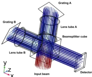
The optical model of the double greating SHS arrangement was constructed in Comsol Multiphysics v5.5, using the geometrical optics interface and the ray tracing module. During the modeling of the sensitivity, free spectral range and time dispersion characteristics of the setup, a parametric sweep of non-sequential ray tracing was performed using hexapolarly arranged, unpolarized, monochromatic and colli- mated input light beam consisting of 331 individual rays, with plane wave approximation. Real reflective grating parameters, taken from the Thorlabs product catalog, were used in the models (150, 300 and 600 mm−1 ruled gratings blazing at 500 nm). The plane of the grating surface was vertically aligned (there was no tilt) and the square-shaped detector was always placed at the same distance from the center of the beams- plitter as the gratings. The fundamental experimental variables of the SHS setup were the grating arm lengths (distance of the center of the grating surface from the active plane of the beamsplitter; varied here as 50, 75 and 100 mm), grating rotation angle (around an axis oriented along the z direction and placed at the grating surface, measured counterclockwise from the grating to beamsplitter optical axis; here varied between 65 and 90 degrees), input beam wavelength, and input beam diameter. Unless stated otherwise, gratings were used in the first diffraction order and the beam diameter as well as the side length of the square-shaped imaging detector was kept at 20 mm. Physics controlled extra fine mesh was used. The visible wavelength range of 400 to 700 nm was considered. A schematic of the Comsol optical model can be seen in Fig. 1. Lens tubes were added to the setup in order to block stray rays, that could otherwise reach the detector via internal reflection on the top and bottom sides of the beamsplitter cube.
2.2. Modeling based on interferometry
For the purposes of modeling the interference pattern, generated by the dual-grating SHS optical arrangement, we developed a Matlab pro- gram, which only uses the core modules of the software. Our calcula- tions were essentially based on the equations published by Harlander at.
al [9], with the difference that we use the exact formula of the Fizeau frequency. The first used equation is the grating formula
σ[sinθ+sin(θ− γ) ] =m
d (1)
where σ is the wavenumber, Θ is the Littrow angle (angle between the optical axis and the normal of the gratings in Littrow configuration),
Fig. 1.Conceptual ray tracing model of the dual grating SHS setup in Comsol.
Please note that the number of rays plotted here is largely reduced for the sake of easy overview.
γ is the diffraction angle of the light component with σ wavenumber, m is the number of the diffraction order and 1/d is the grating density.
The second equation is that of the Fizeau frequency, which can be calculated as
fx(σ) =2σsin(γ) (2)
and describes the spatial frequency of the fringes perpendicular to the x axis. Finally, the third equation used is the interferogram intensity equation
I(x,y) =
∫∞
0
B(σ)⟦1+cos{2π[4fx(σ)x+2ασy] }⟧dσ (3) in which I(x,y) denotes the intensity at the detector image position with horizontal (x) and vertical (y) coordinates, α is the tilting angle difference between the gratings, B(σ) is the spectral density function, and fx (σ) is the frequency of the Fizeau fringes generated by light component with σ wavenumber (see Eq. (2)).
During the calculations it was assumed that the rotation angles of the diffraction gratings are the same and correspond to the Littrow config- uration. In all of our calculations, the Littrow wavelength was set to 500 nm in accordance with the data used in the geometrical optics modeling.
Both gratings were considered not to be tilted, that is their rotation axes were parallel and hence the tilting angle (α) was 0◦. We only considered the first diffraction order.
As is known, in the spectroscopy community there actually is a mixed use of frequency and wavelength representations. Theoretical (physical) processes are described in terms of the frequency (wavenumber), but in the optical practice as well in analytical atomic spectroscopy, which has direct relevance with SH-LIBS that works in the UV–Vis range, the use of wavelengths expressed in nanometers is customary. Specifications of all optical components as well as performance indicators of spectrometers in this field are given in nanometers. As a consequence of this, we also adopted a mixed use of units in this study; interferometric calculations were done in the wavenumber regime, but the performance character- istics of the SHS setup are given in terms of nanometers.
The spectral density function, in other words: the input spectrum, was generated artificially and consisted of several Gaussian peaks, placed at a distance of 100 cm−1 from each other, with identical in- tensity and a 2 cm−1 FWHM. The data vector of the input spectrum consisted of 4n +1 points, where n is the number of the pixels in one row of the applied imaging detector. This oversampling was chosen in order to avoid sampling errors as much as possible.
In order to eliminate ambiguity in the recovered spectra (please note that λ =λ0 +Δλ and λ =λ0 - Δλ generate exactly the same fringe pattern [9,25]) we only kept the upper half of the generated spectrum and also limited the occurring optical components in the input spectrum. The lower limit of the input spectrum were set at the Littrow wavelength (a fixed 500 nm in our study), and the upper limit were defined by the largest possible Fizeau frequency that the number of pixels of the im- aging detector could contain. This numerical situation can be
experimentally easily realized by using a band-pass filter.
The imaging detector and its pixels were always considered to have a square shape. The detector consisted of n pixels in all rows and columns.
The value of n was set as either 256, 512, 1024 or 2048. The physical length of the sides of the detector was set as either 5, 10, 15, 20 or 25 mm in the simulations. In order to avoid problems caused by undersampling, the interferogram intensities were calculated in 4n +1 times 4n +1 overall coordinate positions and the actual intensity of a detector pixel was calculated as the sum of the intensities for 25 gridpoints falling within the boundaries of the given pixel. Subsequently, the gridpoints on the edges and corners contributed to the intensity of more than one detector pixel.
The spectrum was recovered by fast Fourier transformation (FFT).
Since the pixel numbers of the detector were always a power of 2, this process did not require interpolation. The FFT was executed on every row of the interferogram individually and then the row spectra were summed (corresponding to binning), resulting in one single output spectrum per run. The x axis of the output spectrum was calibrated ac- cording to the known position of the first and last spectral peaks in the input.
2.3. Instrumentation
Our study is primarily theoretical, but all calculations were per- formed using the characteristics of actual optical elements, which are used in our experimental SH-LIBS system (here only represented with results shown in Fig. 5).
The system is built around an SM1-threaded Thorlabs 30 mm opto- mechanical cage system [31]. The reflective gratings blazed at 500 nm (Thorlabs No. #GR25–0605 for 600 mm−1, #GR25–0305 for 300 mm−1, etc.) were used and placed in kinematic mounts (Thorlabs KM100S) on top of precision rotation stages with resonant piezoelectric motors (Thorlabs Elliptec 8) equipped with computer control. A 50:50 non- polarizing beamsplitter cube (Thorlabs CCM-BS013/M) was placed in the center of the setup. A mercury‑argon spectral calibration lamp (Ocean Optics Hg-1) was used as calibration light source. The light of this lamp was coupled into the SHS through a 400 μm fiber optic cable (Thorlabs M28L01) and a fiber optic collimator (Thorlabs RC12SMA- F01). A Kiralux 2.3 megapixel monochrome CMOS camera (Thorlabs CS235MU) was used as imaging detector.
3. Results and discussion
Many of the performance features of a LIBS-SHS setup have limita- tions imposed upon the system by both geometric and interferometric conditions. In addition to this, some of the performance features are also interrelated to each other. Thus in the following sections, we will discuss these features in a non-linear way, in which these relationships, and interferometric calculations and geometrical optical simulations are continuously considered and evaluated in parallel.
3.1. Spectral bandpass
From an analytical point of view, the spectral bandpass (SB), and more importantly the free spectral bandpass (FSB, bandpass not influ- enced by diffraction order overlap), of a spectrometer is crucial, because it directly limits the spectral information that can be collected. However, a wider spectral window also dictates the use of an imaging detector with higher pixel resolution in order to maintain an adequately good spectral resolution, which has an especially high importance in atomic spectroscopy. Of course, these conditions also apply to LIBS. It is also worth mentioning that in compact spectrometers, either dispersive or interferometric, the cross-talk of diffraction orders is generally a serious issue, which is typically handled by using order-sorting optical filters or spatial filtering.
In an SHS, geometric conditions as well as interfogram sampling both Fig. 2. Gridpoints within one detector pixel for which the interference pattern
was calculated. The pixel intensity was then taken as the sum of intensities at the gridpoints.
strongly influence the achievable SB. Rules of geometric optics dictate that only those rays of light that reach the detector can contribute to the spectral output. Due to the action of the diffraction gratings, different wavelengths will travel along different pathways within the optical arrangement and hence whether a certain wavelength reaches the de- tector or not, will depend on the grating density, grating rotation, grating blaze wavelength, arm lengths (distance of the detector and gratings from the optical center of the setup within the beamsplitter), beam diameter and detector side length. On the side of interferometric calculations, where geometrical conditions do not come into play, the limitation in SB primarily comes from the fact that the detector side pixel number covered by the beam diameter limits the Fizeau frequency that can be sampled. Thus, interferometry suggests that with regards to SB, the grating blaze wavalength (Littrow wavelength), detector side length and detector pixel number are the most relevant parameters. In the end, the actual (experimental) SB is expected to be the common part (inter- section) of the geometric and interferometric spectral bandpasses. We hereby report about the results of the two optical modelings.
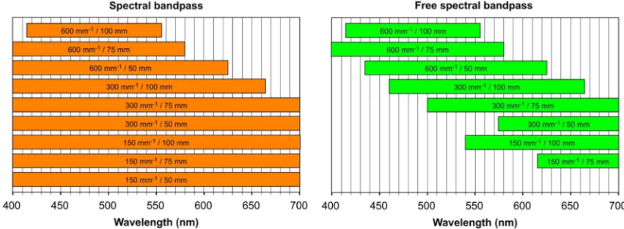
The FSB of the SHS arrangement was estimated by using ray tracing with a parameter sweep for the input beam wavelength (400 to 700 nm) and assessing the range of wavelength in which the first order output at the detector is free from contribution from second order diffraction. The gratings were fixed at their Littrow angle (Θ) and the detector side length was the same as the beam diameter, that is 20 mm. We defined FSB as the wavelength range between the maximum and minimum wavelengths for which the relative sensitivity is at least 10% (here, the sensitivity was represented by the relative number of emitted rays from the light source reaching the detector). As it is shown in Fig. 3, it was found that the SB generally becomes consistently narrower with the increase of the grating density and the arm length. The FSB is always between 100 and 200 nm and is always significantly narrower than the spectral bandpass, except for the 600 mm−1 grating, in which case FSB is equal to SB. The center position of FSB decidedly shifts towards shorter wavelengths with the increase of the two control parameters. FSB is the widest (200 nm) for the 300 mm−1 grating, but is not much narrower for the 600 mm−1 grating with shorter arm lengths. In general, FSB seems to increase with the arm length for less dense gratings, whereas the trend is reversed for the 600 mm−1 grating. These findings indicate that it is generally mandatory to use optical filters in a compact SHS setup, pri- marily for order-sorting purposes, strategically placed at the input. In general, the compact size (short arm length) of an SHS does not seem to be very limiting the FSB, and is comparable to that of linear CCD dispersive spectrometers most often used in LIBS instrumentation with around 0.1 nm or better spectral resolution (these dispersive spec- trometers are similarly compact, with focal lengths in the range of 75 to
100 mm).
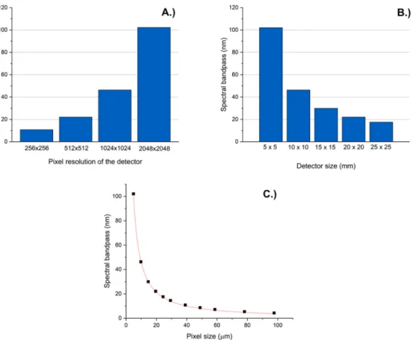
Interferometric calculations were performed for the 300 mm−1 grating, with the Littrow (blaze wavelength) fixed at 500 nm, using different detector side lengths and side pixel numbers. The results can be seen in Fig. 4. It can be directly seen that the SB strongly increases with the number of pixels on each sides of the detector (Fig. 4a, for a given detector side length) and it strongly decreases with the increase of de- tector side length (Fig. 4b., for a given, fixed number of pixels on each sides). This actually suggests that the determining factor is the detector pixel size (pixel side length). Plotting the SB for possible combinations of realistic detector parameters (for pixel numbers from 256 ×256 to 2048
×2048 and for detector side lengths from 5 ×5 mm to 25 ×25 mm), the SB was found to vary according to a power function with negative exponent near one (Fig. 4c). This results is understandable, as in inter- ferometric calculations, SB is limited by the highest Fizeau frequency which can be sampled by the detector, which is in turn related to the physical size of the pixels.
The comparison of the results of the two sets of modeling reveal that in the realistic parameter range, the detector parameters (via Fizeau frequency sampling limitations) have the largest influence on the spec- tral bandpass. Under the conditions tested here for a 300 mm−1 grating, the best SB is around 100 nm (from 500 to 600 nm), which can be ob- tained by using a large pixel number (small pixel size) imaging detector.
Please note that in SHS setups, a small pixel size does not neccessarily gives rise to a decreased sensitivity, due to the fact that each frequency in the spectrum is sampled by multiple pixels located at equidistant interval (multiplex advantage).
3.2. Tuning characteristics
The tuning of an SHS can be achieved by changing the crossing an- gles of the wavefronts, which in practice is done by the rotation of one or both of the gratings along its vertical axis (parallel with the grooves).
When both gratings are rotated, the direction of their rotation must be opposite [1,7]. The tuning (shift of spectral bandpass) is very sensitive to grating rotation. Our experiments indicate that in a typical, compact SHS, a rotation of as small as 0.5 degree already results in a shift com- parable to the total spectral bandpass (Fig. 5).
This tuning however, comes at the expense of the sensitivity as the efficiency of blazed gratings is always largest at the Littrow (rotation) angle, which allows the direction of the reflected rays at the blazing wavelength reflected in the first order to coincide with the incoming rays. Due to this, the tuning characteristics of a double-grating SHS are strongly related to the overall sensitivity of the setup. This is illustrated in Fig. 6, which shows the relative sensivity for three gratings at the 500
Fig. 3. Effect of the grating density and arm length on the spectral bandpass and free spectral bandpass of the SHS arrangement according to ray tracing modeling.
Please note that in the 150 mm−1 / 50 mm case there is no free spectral bandpass, due to the full-range cross-talk between the first and second order of diffraction.
Input beam diameter is equal to the detector side length: 20 mm.
nm blazing wavelength (for the definition of grating rotation angle, please see Section 2.1.) when the two gratings are concertedly rotated (this does not detune the spectrum, but affects grating efficiency). It is apparent that the effect of rotation angle is great on the sensitivity; in the case of the studied conditions, a rotation with only a couple of degrees results in a nearly 50% loss in sensitivity. Please note that the sensitivity
as a function of wavelength follows a more complicated trend (a hint of this can already be seen for the Hg spectral lines in Fig. 5); the discussion of this trend is provided in Section 3.4.
3.3. Spectral resolution
Wavelength calibration of the recovered spectra were carried out by using the position (bin number) and known wavenumber data of the first and last peak of the spectra, using a calibrated Hg line light source. The bin number shows a linear proportionality with the wavenumber, Fig. 4. Effect of the detector parameters (a.) pixel resolution, b.) detector side length, c.) pixel size) on the spectral bandpass, according to interferometric calcu- lations. Square shaped imaging detector, 300 mm−1 grating density, 500 nm blaze wavelength, grating rotation set at the Littrow angle.
Fig. 5. Illustration of the effect of the rotation of one of the gratings on the tuning (shift) of the spectrum, as recorded experimentally, using a Hg–Ar lamp as light source. Grating density: 300 mm−1 Other experimental conditions are similar to the ones used in the simulations of the present study, except that the axes of the two gratings were slightly tilted, which results in the non- redundancy of the observed peaks with the same difference in wavenumber from the center (here located at bin number 512, indicated by the dashed line) [31].
Fig. 6.Effect of the concerted grating rotation on the relative sensitivity of the SHS arrangement, at the blazing wavelength (500 nm), according to ray tracing modeling. Arm lengths are 50 mm. Position of maxima correspond to the Lit- trow angle.
therefore other bin numbers could be easily assigned to wavelengths.
Defining spectral resolution as the bin „width” of the reconstructed spectrum (the minimal detectable wavelength difference) it is possible to evaluate how the various instrumental parameters influence the res- olution. Detector side pixel number, detector side length and the grating density are the most important parameters. As we have shown it above, the first two parameters directly determine the spectral bandpass ac- cording to the interferometric calculations and grating density is known from the experimental SHS literature to have a great influence on the spectral resolution. In addition, we found that the spectral resolution (bin width) is also a function of wavelength. Figs. 7 and 8 illustrate these dependencies. As it can be seen, the wavelength dependence of the resolution is strongest for small detector sizes and small grating den- sities; in case of a 20 or 25 mm detector and at least 600 mm−1 grating densities, this dependence is negligible. The best spectral resolution was in the pm range, but – as it was expected – it came with the expense of the spectral bandpass (ca. 5 nm). This resolution allows LIBS isotope analysis (e.g. the atomic isotope shift for protium and deuterium at the Balmer Hα line is about 170 pm, whereas for 238U and 235U it is about 25 pm at the 424.4 nm U II line).
3.4. Sensitivity
As with all spectrometers, the sensitivity of an SHS also depends on many factors, which is generally represented by the so-called instru- mental function, that is typically a strong function of the wavelength.
Influencing factors include the transmission of optical components, de- tector sensitivity curves, imaging objective distortions, number and area of detector pixels involved in the interferometric sampling, geometric issues, etc. just to name a few. This makes sensitivity the most complex performance feature of the SHS. We studied these factors and their re- lations in detail.
Geometric conditions affecting the sensitivity of the SHS setup were studied via the ray tracing method. In this method, essentially the fraction of rays released from the light source reaching the detector depends on the grating density, rotation angle and grating arm length.
For example, as it can be seen in Fig. 6, the relative sensitivity at the blazing wavelength is maximal at the Littrow angle, as expected. Due to the same blazing wavelength for the real gratings used in the calcula- tions, the blaze angle (and hence Θ) changes linearly with the grating density. The trend is unaffected by the arm length. At one hand, this indicates that according to the expectations, the highest sensitivity can be achieved if the gratings are fixed at Θ.
Another geometric condition affecting sensitivity is the relative size of the input beam and the detector, as well as the wavelength. This is illustrated by Fig. 9. In these ray tracing simulations, we kept the
detector size fixed at 20 mm, the gratings were fixed at their Littrow angle and we varied the other two parameters. As it can be seen, a decrease of the input beam diameter (assuming the same photon flux)
Fig. 7. Effect of a.) the detector side length (for 2048 ×2048 pixel detector) and b.) detector pixel number (for a 10 ×10 mm side length detector) on the spectral resolution (bin width in the output spectrum) as a function of wavelength calculated for gratings with a density of 300 mm−1. Data shown are based on interfer- ometric calculations.
Fig. 8.Effect of the grating density on the spectral resolution (bin width in the output spectrum) as a function of wavelength calculated for a detector of 10 × 10 mm size and 2048 ×2048 pixels. Data shown are based on interferometric calculations.
Fig. 9. Effect of the wavelength and input beam diameter on the relative sensitivity of the SHS arrangement, according to ray tracing simulations. The detector side length is 20 mm, grating density is 600 mm−1, the gratings are fixed at their Littrow angle, arm lengths are 50 mm.
increases the relative sensitivity and makes its wavelength-dependence less pronounced. The reason behind this is that a smaller diffracted beam can be better fully accomodated by the detector than a large beam. At the same time, the decrease of the beam diameter also decreases the spectral coverage. In terms of wavelength, the maximum sensitivity is reached at around the blaze wavelength (500 nm), as expected. A similar trend was observed for other gratings and arm length values as well.
A better comparison of the overall sensitivity of setups with different arm lengths and grating densities can be done via the calculation of the total intensity (cumulative fraction of rays) reaching the detector within the FSB. From the data in Table 1 it is clear that the sensitivity is best for the 300 mm−1 grating, even if the total intensities are normalized with the width of the FSB (cf. Table 1 and Fig. 3). It is a somewhat surprising finding, considering that the blazing wavelength for the gratings used here is 500 nm, and the grating efficiency is known to be greatest around this wavelength, therefore the 600 mm−1 grating, for which the FSB is roughly centered around 500 nm, would be expected to be optimal from the point of view of sensitivity. The reason for this lies in that the wavelength sensitivity curve (fraction of rays reaching the detector) is a maximum curve, and it is becoming more and more narrow as the grating density and/or the arm length increases. Consequently, the
„sweet spot” is in the middle (that is with 300 mm−1), where the loss in sensitivity due to the distance of the center of the FSB from the blazing wavelength is relatively small, but the overall (average) wavelength- dependent sensitivity is still large.
We found interferometric simulations to be also practical for the discussion of the effect of other experimental factors on the sensitivity.
We considered four instrumental conditions here. One was the wavelength-dependence of the sensitivity, namely the wavelength- dependent intensity distortions impacted upon a spectrum (line spec- trum, released from a light source) when it goes through interferometric detection in an SHS. To study this, we used an input model spectrum, which consisted of Gaussian peaks equidistantly placed from each other covering the full FSB (see Section 2.2.). Another objective of our simu- lations was to study the effect of vignetting (reduction of the image’s brightness towards the edges of the image) in the interferogram recor- ded by the detector, often observed in experimental imaging setups. This is usually caused by limitations in the lens, but can also occur if the beam diameter is smaller or equal than the detector side length. This causes a centrally symmetric position-dependent sensitivity envelope, which we represented by a Hanning function in our simulations. A third realistic effect imposed upon the sensitivity is the wavelength-dependent response curve of the detector chip. In the 400–700 nm range, this curve usually has not a high curvature, but within the narrow ca. 100 nm FSB of the SHS arrangements studied here is reasonably flat. We used the actual sensitivity curve of our camera we have in our experimental system as model function during these calculations. The fourth and last factor we discuss is the distortion introduced into the recovered spec- trum if the detector pixel lines (or rows) are binned together in the interferogram, as is conventional in SH spectroscopy to boost S/N, when the other (position and wavelength-dependent) factors above are already in play. This condition also represents the case when the de- tector side length is equal or larger than the beam diameter.
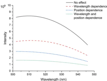
Fig. 10 comprehensively illustrates our findings related to the above factors using the interferometric modeling approach. As it can be seen, the model clearly indicates that even when no explicit instrumental distortions are considered, the sensitivity decreases with the increasing distance from the central (blazing) wavelength. The wavelength- dependent sensitivity is quite apparent in all SHS experiments, where the spectral bandpass is reasonably wide (e.g. in Fig. 5). At the far extreme of the FSB range, the sensitivity is about 50% less than at the other end (at the blazing wavelength of the grating). This behaviour of the sensitivity is probably related to the difference with which an SHS samples different wavelengths (Fizeau frequency). The intensity distortion of the peaks in the detected spectrum is of course further enhanced, if the wavelength- and position-dependent instrumental fac- tors also come into play. Although the extent of the latter two instru- mental conditions is somewhat arbitrary in the model, it can be still noted that their contribution affects (suppresses) the sensitivity far more than the inherent operation of the interferometer. At the same time, these instrumental issues also make the overall instrumental function (sensitivity curve) of the SHS more flat in terms of wavelength.
Finally, we also discuss the dangers of applying pixel binning (line- wise binning) to the interferogram image before FT, if vignetting is present. The distortion of the spectrum is shown in Fig. 11. for three cases: no vignetting, vignetting simulated by the Hanning function, extreme vignetting represented by a round cut-out. The latter case represents a situation when the image does not fill in the square detector (e.g. the beam diameter is smaller than the side length of the detector).
Our simulations revealed that there is a clear and significant distortion in the recovered spectrum if there is vignetting. In the Hanning-function controlled case, the intensities are very strongly affected (suppressed), but the low wavelength end of the spectrum is not distorted. In the case when the vignetting is extremely strong (round-cut image), the situation is the opposite: the overall sensitivity is only slightly lower, but the low wavelength end of the spectrum of seriously distorted. This behaviour is in accordance to the general expectations and it suggests that vignetting has to be avoided in SHS systems. In reality though, it can hardly be avoided – at least not at the expense of other performance characteris- tics, since overfilling the detector with the interferogram image obvi- ously causes a further significant decrease in sensitivity. It therefore seems beneficial to use only the middle section of the interferogram, for
Table 1
Effect of the grating density and arm length on the relative sensitivity (total wavelength-cumulative light reaching the detector) within the respective free spectral bandpass of the given arrangement, based on ray tracing calculations.
The detector size and input beam diameter were both 20 mm in this simulation and the gratings were fixed at their Littrow angle.
Grating density
Arm length 150 mm−1 300 mm−1 600 mm−1
50 mm 0 1803 2569
75 mm 1074 2654 2170
100 mm 1825 2728 1636
Fig. 10.Trendlike effects of wavelength-dependent (camera sensitivity curve) and position-dependent (lens vignetting modeled by a Hanning-function) instrumental distortions of a comb-like input spectrum as detected by the SHS and modeled by interferometric calculations. The graph presents four scenarios: no instrumental effects in action, position-dependent effect, wavelength-dependent effect, and both effects in action. 10 ×10 mm size de- tector with 1024 ×1024 pixels, 300 mm−1 gratings.
which an elongated rectangular 2D detector, or a linear detector array with vertically largely elongated pixels (which is the type used in most dispersive spectrometers to somewhat mirror the proportions of the slit for improved sensitivity), may be a good compromise.
3.5. Light coupling and time dispersion
Interferometry with continuous, coherent light sources is relatively easy. However, when short, broadband (white), non-coherent light pulses serve as the input for an interferometric spectrometer such as the SHS, things can get more complicated. The mode of light input (e.g. free- space or via a fiber optic cable) can also have a significant influence on the interfogram obtained, especially if high time resolution spectroscopy is attempted. This is also the case in SH-LIBS, where a short-living, broadband-emitting microplasma is the light source. Under typical and single-pulse conditions, ns LIBS of a solid sample produces a plasma with a lifetime on the order of some tens of μs (the time-profile of emission line intensities strongly depend on experimental conditions and whether a neutral or ionic line is monitored). If ns LIBS analysis on liquids or fs LIBS on solids is performed, the plasma lifetime is a magnitude shorter, around 1 μs or less [35,36]. LIBS uses gated detec- tion in order to minimize continuum background radiation, hence the required gating width is often one or two orders of magnitude shorter
than the plasma lifetime. The above conditions require a detailed investigation of the dispersion caused by the SHS arrangement as well as the means of coupling of the input light into the interferometer in order to determine the limiting condition and the best potential time resolu- tion of the SH-LIBS system.
First, let us consider the dispersion occurring inside the SHS arrangement itself. Dispersion will mainly occur because rays, depend- ing on their relative position within the beam, will reach the detector at different times due the rotated gratings. In addition, different wave- lengths will also travel through paths of slightly different length. Ray tracing simulation for all our modeled SHS arrangements (all grating variations, fixed at their Littrow angles, varying beam diameters and arm lengths, with wavelengths within the FSB), indicate that the dispersion within the SHS arrangement is always quite small: it varies between 2.4 and 27.9 ps. Table 2 provides an overview of the results. As expected, the dispersion scales linearly with the beam diameter, but the effect of wavelength and grating parameters is complex. Interestingly, the worst dispersion was found within the FSB of the 600 mm−1 grating at the shortest arm length value.
The evaluation of the effect of the means of light coupling into the SHS requires a detailed analysis. One extreme is the free-space coupling (or with minimal optical elements) of the plasma light into the inter- ferometer, which is the case e.g. in stand-off LIBS scenarios [30]. The Fig. 11. Effect of vignetting and binning on the distortion of a comb-like input spectrum as detected by the SHS. Each spectra were recovered from a particular horizontal line of the interferogram image (line number are indicated in the graphs) using FT. The interferometic curves and spectra are shifted vertically to help the eye.
application of fiber optic coupling is expected to deteriorate the time resolution of the LIB-SHS system, because dispersion in an optical fiber results in a distortion of the transmitted short optical pulses. Generally, there are three processes responsible for dispersion. Chromatic (or material) dispersion originates from the fact that the refractive index of the material of the fiber (core) is wavelength-dependent, thus different wavelength components of the light will travel with different speeds.
This effect is proportional to the spectral bandwidth of the source and the length of the fiber. Modal dispersion comes from the pathlength experienced by different rays entering the fiber core at different angles as they travel along. This effect scales with the length and numercial aperture of the optical fiber. The third effect, the so-called waveguide dispersion, is related to the fraction of power coupled into cladding modes, as these modes experience a lower refractive index and hence a different wavelength-dependence than core modes. In large-core multimode fiber optic cables this latter type dispersion is very small thus can be neglected in most cases. The LIB plasma produces a broad- band (white) radiation pulse and is collected in a multimode fiber op- tical cable, thus both modal and chromatic dispersion have to be considered. Graded-index optical fibers have much better, but also more complex, characteristics in terms of modal dispersion, hence here we are only going to discuss these effects for step-index fibers, which are more commonly used in LIBS practice. We will only consider fused silica fibers with the typical 0.22 numerical aperture and 2 m length. We also neglect the temperature-dependence of the contributing effects, and perform the calculations only for room temperature.
Chromatic dispersion is estimated by the following formula
∆tchr= |Dchr|∙L∙∆λ (4)
where Dchr is the chromatic dispersion coefficient, typically given in ps⋅nm−1⋅km−1 units, L is the length of the fiber and Δλ is the spectral bandpass of the light transmitted by the fiber [35]. Depending on the wavelength, Dchr can be both positive and negative, referring to the cases of positive and negative chirp, but here it is adequate to consider only the magnitude of the effect, hence the use of the absolute value function.
The value of Dchr can be calculated by the formula Dchr=λ
c∙d2n(λ)
dλ2 (5)
where λ is the vacuum wavelength, c is the speed of light and n(λ) is the wavelength- dependent refractive index, usually represented by the Sellmeier function
n(λ)2=A+ B 1− C/
λ2+ D 1− E/
λ2 (6)
where the A, B, C, D, E constants are all related to physical processes and are determined by fitting of the experimental data [38]. In our calcu- lations, we used the Sellmeier coefficients published by Ghosh et al. for fused silica [39]. From the above formulas, it is obvious that Dchr is wavelength-dependent, through n(λ). The formulas give values of 2.33 ps and 0.38 ps (per nm and per 2 m) for Dchr as for the two extreme wavelengths of 400 and 700 nm, respectively. Due to the significant spectral bandpass of SHS arrangement (up to about 200 nm with certain parameter combinations) the simple approximation of multiplying Dchr
with the wavelength range to assess the chromatic dispersion in unit fiber length would not be accurate, therefore we calculated aggregated dispersion with 1 nm resolution for all FSB wavelength ranges sepa- rately. See Table 3 for the values obtained. We would like to point out to that the typical assumption that the chromatic dispersion is much smaller than the modal dispersion [37] does not hold here in most cases – the reason is the significant wavelength range (FSB) in which the SHS arrangement operates as opposed to the narrow bandpass used in tele- communication or optochemical sensor applications. It should also be noted that chromatic dispersion causes temporal redistribution of different wavelength components within the pulse (with shorter being in the front and longer in the rear of the pulse, or vice versa, depending on the sign of Dchr). As a consequence, the arm length should be set equal with higher precision in order to have the same wavelength components to arrive at the detector simultaneously.
The modal dispersion in a step-index fiber is usually approximated by
∆tmod≈ L∙NA2
2∙c∙ncore (7)
where L is the length of the fiber in meters, NA is the numerical aperture of the fiber and ncore is the refractive index of the core material of the fiber [35]. Let us fix these costants at their typical value, which is NA = 0.22 and ncore ≈1.46 for fused silica in the visible range. This gives a value of 110.58 ps. This value is also indicated in Table 3, along with the total (chromatic + modal) value of the dispersion. Clearly, the total dispersion in the optical fiber can be minimized by keeping the fiber length and the NA as small as possible (please also note that as it was alluded to above, graded-index fibers have significantly improved dispersion characteristics).
It should be mentioned that dispersion also occurs during the coupling of the plasma emission into the optical fiber and also at the collimation of the light output from the fiber. For the sake of simplicity, let us assume a two-lens light collection arrangement at the fiber input Table 2
Dispersion (time difference between various rays reaching the detector) in the SHS arrangement, as evaluated by ray tracing simulations for (amost) all experimental parameter combinations. Grating rotation angle was fixed at the respective Littrow angle. The effect of the beam diameter was only tested with the 150 mm−1 grating and at the 500 nm blaze wavelength.
Grating density (mm−1)
Wavelength
(nm) Beam
diameter (mm)
Arm length
(mm) Dispersion (ps)
150 500 5 50 2.4
150 500 10 50 4.6
150 500 15 50 7.0
150 500 20 50 9.4
150 615 20 75 6.3
150 700 20 75 4.4
150 540 20 100 7.3
150 700 20 100 2.9
300 575 20 50 17.9
300 700 20 50 10.1
300 500 20 75 19.1
300 700 20 75 4.3
300 460 20 100 13.5
300 665 20 100 3.0
600 435 20 50 27.9
600 625 20 50 6.4
600 400 20 75 9.6
600 580 20 75 5.8
600 415 20 100 5.7
600 555 20 100 6.8
Table 3
Chromatic, modal and total dispersion values for a fused silica step-index optical fiber (NA =0.22, length =2 m) in the FSB spectral windows for the indicated grating density and arm length combinations (as per Fig. 2).
Grating density (mm−1)a
Arm length (mm)
Chromatic
dispersion (ps) Modal dispersion (ps)
Total dispersion (ps)
150 75 39.69 110.58 150.27
150 100 92.14 110.58 202.72
300 50 64.93 110.58 175.51
300 75 131.15 110.58 241.73
300 100 167.71 110.58 278.29
600 50 188.26 110.58 298.84
600 75 232.04 110.58 342.62
600 100 180.91 110.58 291.49
and single lens collimation at the output, with identical lenses NA- matched to the fiber, and neglect the dispersion occurring in the len- ses, which are very thin compared to the length of the fiber (hence we also neglect chromatic aberration). In this scenario, the dispersion due to the different path lengths the light travels through the lenses will be proportional to the beam diameter. In total (considering all three len- ses), the calculation gives 1.89 ps, 3.79 ps, 5.68 ps and 7.58 ps values for 5, 10, 15 and 20 mm beam diameters. As expected, these values are only a couple of percents of and therefore neglectable compared to the total dispersion occurring in the optical fiber.
Overall, it can be stated that the dispersion of pulsed light in the SHS arrangement alone is very small compared to the dispersion that occurs in the optical fiber, if the LIB plasma emission is coupled into the SHS arrangement via a fiber. In this case, the shortest gate width that can be used at the imaging detector is about 0.2–0.4 ns. If the time resolution of the SH-LIBS system is of a concern and sensitivity is not limiting, then free-space light coupling can be advised. Otherwise, keeping the NA and length of the optical fiber low as well as using experimental parameters resulting in a smaller SB can help to minimize the dispersion.
4. Conclusions
We carried out extensive ray-tracing simulations and interferometric calculations to provide a detalied characterization of the potential spectroscopy performance of LIBS systems incorporating an SHS spec- trometer. A number of experimental parameters were tested and several relative figures of merit were calculated.
We have shown that the tuning of the SHS by rotating the gratings is technically relatively straightforward and it is very effective. A rotation of a fraction of a degree is sufficient to shift the measurable wavelength window by nearly its full bandwidth. It is an advantage of this spec- trometer that such a slight rotation does not greatly influence either the sensitivity or the width of the spectral window. However, this also means that the setup is sensitive to misalignments and vibrations, thus a permanently aligned, rigid construction is preferable.
A 100 nm free spectral bandpass (measurable wavelength window, free from diffraction order overlap) is achievable with a compact (50–100 mm arm length) SHS arrangement. It was found that the in- fluence of detector pixel size is stronger on this than that of geometrical conditions. The typical, ca. 5 μm, pixel size of most megapixel imaging detector chips in use today is adequate for a relatively wide, 100 nm spectral bandpass with a spectral resolution better than 100 pm, adequate for general LIBS use.
The spectral resolution was found to be strongly depending on the wavelength, but our simulations clearly showed that it is feasible to achieve a better than 50 pm spectral resolution with a compact SHS equipped with a megapixel imaging detector and at least medium line density (≥1200 mm−1) gratings. The best resolution was estimated to be about 10 pm (with a spectral bandpass of about 5 nm), which is quite adequate even for isotope selective measurements in an evacuated laser ablation cell.
Although the literature generally outlines the sensitivity of an SHS as mainly depending on the grating density (lower density gratings should give rise to a higher sensitivity), but our simulations revealed that the (relative) sensitivity of the SHS is a complex function of conditions.
Essentially all instrumental parameters, as well as the distance of the analyte line from the lower end of the spectral bandpass, were found to have a profound effect on the sensitivity. Sensitivity optimization is therefore difficult, but not impossible and requires sophisticated simu- lation tools. We also made observations as to how line binning of the interferogram image, which is an often exercised technique to improve S/N, can distort the spectrum, if a realistic experimental system burdened with optical vignetting and wavelength-dependent imaging detector sensitivity is used.
Finally, we also investigated the effect of light in-coupling mode (free-space or via fiber optics) on the time dispersion of the whole SHS
system, considering the spectral bandpass calculated above. Time dispersion is relevant for SH-LIBS setups because it directly influences the shortest gate width applicable, especially if short liftime (e.g. fs laser generated) laser-induced breakdown plasmas are studied. Our calcula- tions revealed that the time dispersion occurring in a compact SHS system amounts to only a few tens of ps, which is a negligible value to the total (chromatic +modal) dispersion related to an optical fiber (up to 400 ps in a 2 m optical fiber). These results suggest that SHS detection is not only applicable in ns, but also in fs LIBS systems.
Our work provides theoretical (simulational) evidence that SHS has a great potential for use in LIBS systems, as well as it outlines the ap- proaches through which the optimization of SH-LIBS systems is possible.
Declaration of Competing Interest
There are no conflicts of interests to declare.
Acknowledgments
The financial support received from various sources including the Ministry of Innovation and Technology (through project No. TUDFO/
47138-1/2019-ITM FIKP and TKP 2020) and the National Research, Development and Innovation Office (through projects No. K_129063, EFOP-3.6.2-16-2017-00005) of Hungary are kindly acknowledged. D.J.
Palasti also wishes to thank the grant he received from the ÚNKP-20-3 - ´ New National Excellence Program of The Ministry for Innovation and Technology of Hungary financed by the National Research, Develop- ment and Innovation Fund. The open access publication of this work has been supported by the University of Szeged Open Access Fund, under Grant No. 5389.
References
[1] A.P. Thorne, M.R. Howells, Interferometric Spectrometers, Chapter 4 in the Experimental Methods in Physical Sciences Series Vol. 32, Academic Press, 1998.
[2] P. Hariharan (Ed.), Basics of Interferometry 2nd Ed, Academic Press, Cambridge, 2007.
[3] P.B. Fellgett, On the ultimate sensitivity and practical performance of radiation detectors, J. Opt. Soc. Am. 39 (1949) 970–976.
[4] P. Jacquinot, How the search for a throughput advantage led to Fourier transform spectroscopy, Infrared Phys. 24 (1984) 99–101.
[5] Y. Xu, X. Wei, Z. Ren, K.K.Y. Wong, K.K. Tsia, Ultrafast measurements of optical spectral coherence by single-shot time-stretch interferometry, Sci. Rep. 6 (2016) 27937.
[6] T. Dohi, T. Suzuki, Attainment of high resolution holographic Fourier transform spectroscopy, Appl. Opt. 10 (1971) 1137–1140.
[7] J.M. Harlander, Spatial heterodyne spectroscopy: interferometric performance at any wavelength without scanning, PhD Thesis, Univ. of Wisconsin, Madison, USA, 1991.
[8] A.B. Gojani, D.J. Pal´asti, A. Paul, G. Galb´acs, I.B. Gornushkin, Analysis and classification of liquid samples using spatial heterodyne Raman spectroscopy, Appl.
Spectrosc. 73 (2019) 1409–1419.
[9] J.M. Harlander, R.J. Reynolds, F.L. Roesler, Spatial heterodyne spectroscopy for the exploration of diffuse interstellar emission lines at far-ultraviolet wavelengths, Astrophys. J. 396 (1992) 730–740.
[10] N.G. Douglas, Heterodyned holographic spectroscopy, Publ. Astron. Soc. Pac. 109 (1997) 151–165.
[11] O.R. Dawson, W.M. Harris, Tunable, all-reflective spatial heterodyne spectrometer for broadband spectral line studies in the visible and near-ultraviolet, Appl. Opt. 48 (2009) 4227–4238.
[12] S. Hosseini, Characterization of cyclical spatial heterodyne spectrometers for astrophysical and planetary studies, Appl. Opt. 58 (2019) 2311–2319.
[13] S. Fransden, N.G. Douglas, H.R. Butcher, An Astronomical Seismometer, Astron.
Astrophys. 279 (1993) 310–321.
[14] T. Nathaniel, Spatial heterodyne Raman spectroscopy, PhD Thesis, University of Surrey, Guildford, UK, 2011.
[15] N.R. Gomer, C.M. Gordon, P. Lucey, S.K. Sharma, J.C. Carter, S.M. Angel, Raman spectroscopy using a spatial heterodyne spectrometer: proof of concept, Appl.
Spectrosc. 65 (2011) 849–857.
[16] M. Kaufmann, F. Olschewski, K. Mantel, O. Wroblowski, Q. Chen, J. Liu, Q. Gong, D. Wei, Y. Zhu, T. Neubert, H. Rongen, R. Koppmann, M. Riese, On the assembly and calibration of a spatial heterodyne interferometer for limb sounding of the middle atmosphere, CEAS Space J. 65 (2019) 525–531.
[17] B. Solheim, S. Brown, C. Sioris, G. Shepherd, SWIFT-DASH: spatial heterodyne spectroscopy approach to stratospheric wind and ozone measurement, Atmos.- Ocean. 53 (2015) 50–57.
[18] J.A. Langille, D. Letros, D. Zawada, A. Bourassa, D. Degenstein, B.J. Solheim, Spatial heterodyne observations of water (SHOW) vapour in the upper troposphere and lower stratosphere from a high altitude aircraft: modelling and sensitivity analysis, J. Quant. Spectrosc. Radiat. Transf. 209 (2018) 137–149.
[19] M.J. Egan, S.M. Angel, S.K. Sharma, Standoff spatial heterodyne Raman spectrometer for mineralogical analysis, J. Raman Spectrosc. 48 (2017) 1613–1617.
[20] Y. Feng, Q. Bai, Y. Wang, B. Hu, S. Wang, Theory and method for designing field- widened prism of spatial heterodyne spectrometer, Acta Opt. Sin. 32 (2012) 1030001.
[21] G. N´emeth, A. Pekker, New design and calibration method for a tunable single- ´ grating spatial heterodyne spectrometer, Opt. Express 28 (2020) 22720.
[22] J.M. Harlander, J.E. Lawler, J. Corliss, F.L. Roesler, W.M. Harris, First results from an all-reflection spatial heterodyne spectrometer with broad spectral coverage, Opt. Express 18 (2010) 6205–6210.
[23] B. Xiangli, Q. Cai, S. Du, Large aperture spatial heterodyne imaging spectrometer:
principle and experimental results, Opt. Commun. 357 (2015) 148–155.
[24] C.P. Perkins, J.P. Kerekes, M.G. Gartley, Spatial heterodyne spectrometer:
modeling and interferogram processing for calibrated spectral radiance measurements, Proc. SPIE 8870 (2013) 88700L.
[25] M. Lenzner, J.C. Diels, Concerning the spatial heterodyne spectrometer, Opt.
Express 24 (2016) 1829–1839.
[26] A. Waldron, A. Allen, A. Col´on, J.C. Carter, S.M. Angel, A monolithic spatial heterodyne Raman spectrometer: initial tests, Appl. Spectrosc. 75 (2021) 57–69.
[27] K.A. Strange Fessler, A. Waldron, A. Col´on, J. Chance Carter, S. Michael Angel, A demonstration of spatial heterodyne spectrometers for remote LIBS, Raman spectroscopy, and 1D imaging, Spectrochim. Acta, Part B 179 (2021) 106108.
[28] G. Galb´acs, A critical review of recent progress in analytical laser-induced breakdown spectroscopy, Anal. Bioanal. Chem. 407 (2015) 7537–7562.
[29] I.B. Gornushkin, B.W. Smith, U. Panne, N. Omenetto, Laser-induced breakdown spectroscopy combined with spatial heterodyne spectroscopy, Appl. Spectrosc. 68 (2014) 1076–1084.
[30] P.D. Barnett, N. Lamsal, S.M. Angel, Standoff laser-induced breakdown spectroscopy (LIBS) using a miniature wide field of view spatial heterodyne
spectrometer with sub-microsteradian collection optics, Appl. Spectrosc. 71 (2017) 583–590.
[31] A. Allen, S.M. Angel, Miniature spatial heterodyne spectrometer for remote laser induced breakdown and Raman spectroscopy using Fresnel collection optics, Spectrochim. Acta, Part B. 149 (2018) 91–98.
[32] D.J. Pal´asti, L. Himics, T. V´aczi, M. Veres, I.B. Gornushkin, G. Galb´acs, Optical modeling of spectroscopic characteristics of a dual-grating tunable spatial heterodyne LIBS spectrometer, 10th Euro-Mediterranean Symposium (EMSLIBS), Brno (Czechia) (2019) 111–112. Presentation #PI_010.
[33] D.J. Pal´asti, M. Veres, I. Rig´o, Zs. Geretovszky, ´E. Kov´acs-Sz´eles, A.B. Gojani, I.
B. Gornushkin, G. Galb´acs, Optimization and detailed spectroscopic characterization of an improved spatial heterodyne laser-induced breakdown spectroscopy setup, in: 2019 European Winter Conference on Plasma Spectrochemistry (EWCPS-2019), Pau (France), 2019. Presentation #WP-42.
[34] M. Lenzner, C. Feng, J. Diels, Resolving isotopic emission lines using a spatial heterodyne spectrometer, in: 17th International Conference on Transparent Optical Networks (ICTON), Budapest (Hungary), 2015, pp. 1–4.
[35] A. De Giacomo, M. Dell’Aglio, O. De Pascale, M. Capitelli, From single pulse to double pulse ns-laser induced breakdown spectroscopy under water: elemental analysis of aqueous solutions and submerged solid samples, Spectrochim. Acta Part B. 62 (2007) 721–738.
[36] B. Le Drogoff, J. Margot, M. Chaker, M. Sabsabi, O. Barth´elemy, T.W. Johnston, S. Laville, F. Vidal, Y. von Kaenel, Temporal characterization of femtosecond laser pulses induced plasma for spectrochemical analysis of aluminum alloys, Spectrochim. Acta, Part B. 56 (2001) 987–1002.
[37] C.A. Bunge, M. Beckers, B. Lustermann, C.-A. Bunge, Basic principles of optical fibres, in: T. Gries, M. Beckers (Eds.), Polymer Optical Fibres Chapter 3, Woodhead Publishing, Cambridge, 2017.
[38] H. Xie, Z.C. Wang, J.X. Fang, Study of material dispersion in amorphous silica optical fibers, Phys. Status Solidi 96 (1986) 483–487.
[39] G. Ghosh, M. Endo, T. Iwasalu, Temperature-dependent sellmeier coefficients and chromatic dispersions for some optical fiber glasses, J. Lightwave Technol. 12 (1994) 1338–1342.