The possibilities of biodiversity monitoring based on Hungarian Light Trap Networks

THE POSSIBILITIES OF BIODIVERSITY MONITORING BASED ON HUNGARIAN LIGHT TRAP NETWORKS

GIMESI,L.¹*–HUFNAGEL,L.²

1University of Pécs, Faculty of Natural Sciences, Department of Informatics H-7624Pécs, 6 Ifjúság Road, Hungary

(phone: +36-72-503-600; fax: +36-72-503-697)

2”Adaptation to Climate Change” Research Group, Hungarian Academy of Sciences H-1118 Budapest, Villányi út 29-43., Hungary

*Corresponding author e-mail: gimesi@ttk.pte.hu

(Received 16^th November 2010 ; accepted 19^th November 2010)

Abstract Our method is presented with displaying time series, consisting of the daily amount of precipitation of 100 years, which has meant a separate challenge, as the precipitation data shows significant deviations. By nowadays, mankind has changed its environment to such an extent that it has a significant effect on other species as well. The Lepidoptera data series of the National Plant Protection and Forestry Light Trap Network can be used to justify this. This network has a national coverage, a large number of collected Lepidoptera, and an available, long data series of several years. For obtaining information from these data, the setting up of an easy to manage database is necessary. Furthermore, it is important to represent our data and our results in an easily analysable and expressive way. In this article the setting up of the database is introduced, together with the presentation of a three dimensional visualization method, which depicts the long-range and seasonal changes together.

Keywords: biodiversity, monitoring, data mining, Lepidoptera

Introduction

The spreading and the structure of ecological associations significantly depend on environmental factors and resources. This is called ecological niche, which can be perceived as part of an n dimensional space that is used by the given population (n dimension means the n number of different environmental effects and resources).

There is no opportunity on an examination of population dynamics to investigate all (n) environmental factors. Therefore we only looked for relationships between a few relevant environmental parameters and the data collected by monitoring the communities. In view of these correlations we attempted to draw conclusions about the future state of the population.

The size and the structure of populations are influenced by several factors:

agriculture, urbanization, climate, soil, vegetation, solar radiation, etc. However, these effects are not independent from each other. Climate change has an effect on each component. Thus, environmental effects (biotic and abiotic), cannot be examined independently from each other. That is, no such ideal circumstances can be created, where it could be investigated for example how the population is effected by temperature changes, since it has an effect on other influential environmental factors as well, which can have an effect on the investigated population. The investigation is further complicated by the fact that climate is not the only thing having an effect on the population and its surroundings. Primarily human activity should be mentioned here.

One of the big problems of these times is that the data available for us are growing at an incredible pace. Filtering out important data from the databases is getting to be an increasing problem.

The aim of our work is to create a database from the Lepidoptera data of the light trap network, which assures the availability of data for the purpose of writing this article and further researches in an easily manageable form. Besides this we have introduced a three-dimensional depicting method in this article, which presents time series figures in an expressive way.

A Visual-Basic program has been made for data processing, evaluating and visualizing the results. We chose this programming language primarily because it can easily be set up for the direct use of Excel and Access files. These programs are suitable for the graphical visualization of long time series with the help of Autocad and ArcGIS graphical programs.

Review of literature

The most widespread collection method of Lepidoptera flying at night is light trapping. This method was first employed following the experiments of Williams (1935). Light traps have been used since 1940 in Hungary. In 1952 the construction of an internationally unique trap network began (Jermy, 1961; Nowinszky, 2003a). By now, the Hungarian light trap system has been equipped uniformly with Jermy type light traps.

Those light traps that have been operating for a long time uninterrupted, in the same place are the most suitable for population dynamics investigation (Nowinszky, 2003b).

It is practical to use all the light trap data because of the effects of different abiotic factors. This way it is achievable that the effects appearing in different collection places and modifying the number of collections neutralize each other (Nowinszky, 2003b).

The longest possible time series (daily data series) is needed to define the changes in a data series and its tendencies in the most reliable way. It should cover the largest possible geographical area and data collection should be carried out with the same method all along. The data series of the National Plant Protection and Forestry Light Trap Network is the most adequate for these conditions (Hufnagel et al., 2008).

Large quantity data coming from different sources can be processed with methods of data mining. As a first step data warehouses are created from databases (Böhlen, 2003;

Fan, 2009; Han and Kambel, 2004; Keim, 2004). This procedure is preprocessing (Kennedy, et al. 1998; Pyle, 1999), during which the automatically detectable defective data are removed. The rest of the defective data can be filtered out only with human assistance, in an interactive way (Han and Kambel, 2004).

With the joining of databases a data structure is created, which ensures data access according to several points of view. The most suitable structure for this is an n- dimensional data cube (Euler, 2005; Gray et al., 1997).

The moving average method can be used for filtering out extremes appearing in databases and for decreasing the fluctuations in data series (Heuvelink and Webster, 2001). It smoothes the data series at the same time(Han and Kambel, 2004).

Image visualization is closer to human thinking than large tables containing numerical data, which, though, provide exact information, but are difficult to handle and they are not suitable to present correlations (Gimesi, 2004) either. When analysing

calculation results, it can be helpful if the data is presented in an easily interpretable, graphical form.

We used three-dimensional figures for the presentation of long time series, where the yearly and seasonal changes could be seen well – these are outlined by Gimesi (2009).

A similar depicting method was used by Mulligan (1998) for the demonstration of the seasonal changes of vegetation. He remarked that the method is able to demonstrate both short- and long-range tendencies. For the demonstration of Lepidoptera data, three- dimensional figures were also used by Marchiori and Romanowski (2006).

Diversity indices are numerical functions defined on sets of species frequency or species occurence probability(Izsák, 2001). So the diversity of a biozoenosis – in an ecological sense – is some kind of a function of the number and abundance of species.

Biological diversity primarily means the variousness of species regarding a given area and a given period. Species, genus or genetic diversities can be studied, such as epidemiologic or population diversities (Izsák, 1994; Izsák and Juhász-Nagy, 1984).

However, diversity indices do not provide information about the spatial position of entities, which can characterize the community at least as much as the number of species or the diversity (Menhinick, 1962).

In statistical ecology numerous functions are applied as diversity indices (Dewar and Porté 2008; Izsák, 2001; Mishra et al., 2009; Sipkay et al., 2005; Tóthmérész, 1997).

Different diversity indices described in the ecological literature present the diversity of a given species community from different points of view. It is general experience that the diversity of numerous fauna and flora communities measured by different indices show significant positive correlation. The main reason for this is the high sensibility of indices to the change of population with the largest number of entities. Indices depend on the size of the sample, though to different extent (Ibáňez et al.,1995).

Numerous methods have been worked out to characterize diversity, which can be assorted as follows, according to Tóthmérész ( 2001):

− Number of species,

− Diversity indices,

− Classical diversity statistics,

− Scale-pending characterization of diversity,

− Mosaicity, the role of patterns (β-diversity),

− Space-series analysis.

Shannon diversity index is the most commonly used in ecological literature (e.g.:

Arnan et al., 2009; Balog et al., 2008; Chefaoui and Lobo, 2008; Kevan, 1999; Skalskia and Pośpiech, 2006), therefore we also investigated the distribution of collected Lepidoptera with the help of this one.

Table 1. Trap statistics (highlighted traps worked for the longest time)

Date Trap Code

Start End

Operation Time [months]

Number of Individuals

Number of

Species Name of Trap

1 Nov. 1961. Dec. 1975. 139 63948 572 Budakeszi

2 Jun. 1961. July. 1991. 302 602476 798 Makkoshotyka

3 Jun. 1961. Dec. 2006. 441 285752 776 Felsőtárkány

4 Apr. 1962. Dec. 2006. 421 291694 677 Gerla-Gyula

5 Jan. 1962. Apr. 1976. 147 29852 60 Kunfehértó

6 Apr. 1965. Oct. 1990. 185 134303 588 Farkasgyepű

7 Jun. 1961. Dec. 2006. 364 102903 662 M.Háza,M.Almás

8 Mar. 1962. Nov. 2006. 417 298604 686 Répáshuta

9 Feb. 1962. Oct. 2006. 393 193967 770 Sopron

10 Aug. 1967. Jun. 1973. 45 11267 416 Szakonyfalu

11 Jan. 1961. Dec. 2006. 354 301795 697 Szentpéterfölde

12 Mar. 1962. Feb. 1977. 153 39242 520 Szombathely

13 Jun. 1961. Dec. 2006. 403 325227 689 Tolna

14 Mar. 1962. Oct. 2006. 445 715915 696 Tompa

15 Feb. 1962. Nov. 2006. 446 476072 765 Várgesztes

16 Jun. 1969. Aug. 1990. 149 25183 479 Gyulaj-Kocsola

17 Aug. 1969. Dec. 2006. 334 175334 698 Erdősmecske

18 Aug. 1969. Aug. 2003. 85 48671 552 Kömörő

19 Aug. 1969. Aug. 1975. 48 578 33 Kőkút

20 Sept. 1969. Jun. 1974. 28 1125 30 Alsókövesd

21 Mar. 1970. Aug. 1975. 45 1656 30 Zalaerdőd

22 July. 1972. Aug. 1995. 204 82770 621 Piliscsaba

23 May. 1978. Nov. 2006. 186 200144 638 Gilvánfa-Sumony

24 Sept. 1977. Dec. 2006. 243 557826 638 Kapuvár

25 Aug. 1976. Sept. 1995. 152 87831 458 Karcag-Apavára

26 July. 1976. Dec. 2006. 253 326855 656 Bugac

27 July. 1976. Nov. 2006. 253 183090 672 Nagyrákos-Szala

28 Jun. 1976. Oct. 2003. 147 68158 538 Szulok

29 May. 1976. Aug. 1985. 72 41544 526 Zalaszántó-Supr

30 Sept. 1975. Nov. 2006. 215 183190 675 Sárvár-Baj-Acsád

31 Mar. 1988. Oct. 1990. 23 6080 62 Bejcgyertyános

32 1977. Apr. July. 2006. 268 161841 618 Sasrét

33 Sept. 1979. Nov. 2000. 188 190769 548 Jánkmajtis

34 May. 1990. Nov. 2006. 154 151071 560 Diósjenő

35 Apr. 1992. Jun. 1995. 14 1785 141 Nagylózs

36 Mar. 1992. Oct. 1998. 38 19153 394 Telkibánya

37 Sept. 1975. Dec. 2006. 141 108785 493 Hőgyész-Tamási

38 Mar. 1981. July. 1981. 5 1183 159 Ivánc

40 Mar. 1977. Sept. 2003. 128 181664 568 Ásotthalom

41 May. 1993. May. 1993. 1 39 18 Gödöllő

42 July. 1976. July. 1979. 26 3094 301 Nádasd

43 Jun. 1977. Aug. 1977. 3 457 54 Albertirsa

52 Sept. 1991. Nov. 2006. 133 204087 702 Bakonybél-Somh

53 May. 1994. Dec. 1995. 13 9468 313 Mosonmagyaróár

54 Dec. 1993. Oct. 1995. 15 4285 195 Ásványráró

55 Mar. 1995. May. 2001. 49 24170 368 Barcs-Krigóc

56 Apr. 1993. Oct. 2006. 109 117965 510 Egyházaskesző

57 Apr. 1996. Oct. 2006. 48 53304 434 Kecskemét

58 Apr. 1996. Nov. 2003. 57 58244 517 Pilismarót

59 Apr. 1995. Dec. 2006. 93 136481 459 Püspökladány

60 Mar. 1999. Nov. 2006. 71 29617 466 Kemencepatak

61 Apr. 1999. Sept. 1999. 6 6322 195 Maroslele

62 Mar. 2005. Aug. 2006. 12 15209 289 Csöprönd

63 Mar. 2005. Sept. 2006. 16 21667 335 Szentendre

64 Apr. 2005. Dec. 2006. 17 35804 365 Vámosatya

Materials and methods

In the course of our work we used the National Plant Protection and Forestry Light Trap Network, the first light traps of which were installed in 1961 (Szontagh, 1975).

These traps are operating all year round, except for those days when the temperature does not rise above 0 °C, or when the area is covered by snow (Nowinszky, 2003a).We received the data of the National Plant Protection and Forestry Light Trap Network in dBase format. Our object was to create a database out of these hardly processable data that allows access to the data easily, in a general format. This way we have created a database essential for further researches.

The data of the National Plant Protection and Forestry Light Trap Network were processed using data-mining methods. As a first step – based on a method well known in the literature(Böhlen, 2003; Fan, 2009; Han and Kambel, 2004; Keim, 2004) – we created a data warehouse out of the available databases. This process included the merge and the filtering of databases (Bogdanova and Georgieva, 2008).

The trap statistics created from the trap data can be seen in Table 1. In this table the beginning and the end of the operation are shown, together with the operation time in months, the total number of collected individuals, the number of collected species, and the name of the trap (its geographical position).

The merge of databases

The original (light trap collection) data can be found in separate databases for each trap. The record structure of the original databases can be seen in Fig. 1.

SORSZ CSAPDA K_KOD A_EV A_HO D1 D2 Data

..

D31 FELV FIDO JEL IDO .. .

. .

. .

. .

. .

. .

. .

. .

. .

. .

. .

.

Figure 1. The record structure of the original databases

The following fields can be found in the databases:

SORSZ (sn) – ordinal number of the measurement CSAPDA (trap) – trap code

K_KÓD (l_code) – code of the insect species( Lepidoptera) A_EV (yoh) – year of collection

A_HO (moh) – month of collection

D1-D30 – number of individuals collected daily FELV (rec) – name of the data recorder

FIDO (torec) – date of recording JEL (sign) – sign

IDO (time) – date of collection

Fig. 2 presents the record structure of trap and species databases. These are linked to the structure presented in Fig. 1.

.. .

. .

. .

. .

. .

. .

. Species

Trap

K_KOD K_NEV K_RNEV KONYV CS_KOD CS_NEV MENT

Figure 2. The record structure of trap and species databases

The following fields can be found in the databases:

CS_KOD (trap) – trap code

CS_NEV (name) – name of the trap MENT – one boolean data

K_KOD (species) – species code K_NEV (name) – name of the species K_RNEV (name) – short name KONYV (name) – name by book

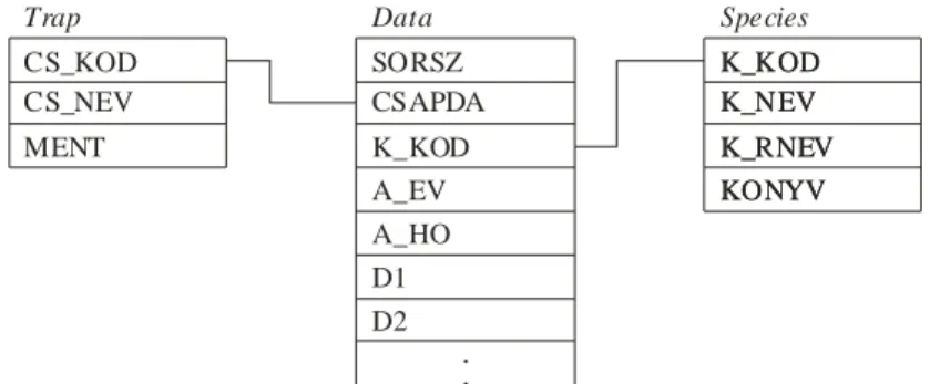
Fig. 3. demonstrates the relational connections of tables (records) presented in Fig.1, Fig. 2.

CS_KOD CS_NEV MENT

SORSZ CSAPDA K_KOD A_EV A_HO D1 D2

..

K_KOD K_NEV K_RNEV KONYV

Trap Data Species

K_KOD K_NEV K_RNEV KONYV

Figure 3. The relational connections of data-tables

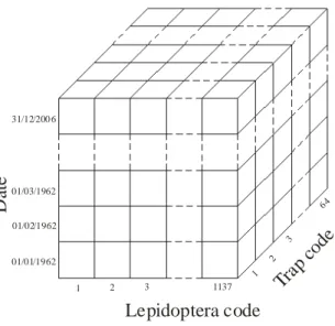
With the merge of databases we created a data structure that ensures searching by trap code, Lepidoptera code, and date. The most suitable structure for this is the three- dimensional data cube that can be seen in Fig. 4. The dimensions of the cube are: time, trap code, species code. This way one elemental cube contains the number of species collected in a given trap on a definite day.

For the sake of quicker data access and the following graphical depiction we have divided the time dimension into year and day. Therefore we actually used a four- dimensional data cube.

While defining the ordinal number of the day – for the sake of uniformization – years were considered to contain 365 days, i.e. measurements made on 29^th February were excluded. This did not cause any error, as during the 45-year period of investigation – considering all the traps and species – it meant leaving out altogether 109 individuals.

Lepidoptera code

Trap code

Date

01/01/1962 01/02/1962 01/03/1962 31/12/200 6

1 2

3 64

1 2 3 1137

Figure 4. The data cube

Data filtering, data cleaning

During the course of creating the data warehouse we executed an automatically performable filtering, during which:

− incorrect dates coming from data recording mistakes were removed (only the data of the period between 1962 and 2006 were collected, the ordinal number of months had to be between 1 and 12, and the number of days had to correspond with the value belonging to the given month),

− those species codes that were not included in the species database have been filtered out,

− doubly recorded data were deleted.

The filtering out of other defective data can be executed in an automatic way only to a limited extent. In the rest of the cases an interactive (requiring human assistance) filtering can be carried out (Han and Kambel, 2004). The visualization method recited in this article is suitable for noticing flagrant (widely differing from the environment) data easily (Gimesi, 2008).

Filtering based on trap code

Those light traps that have been operating in the same place for a long time without interruption are the most suitable for the purpose of investigating population dynamics (Nowinszky, 2003b). Accordingly, we chose from the database those traps have worked for the longest time, mindful of having data of the highest possible number of days in the examined period. We have chosen those 9 traps that worked for the longest time between 1962 and 2006. The data of these are marked with highlighting in Table 1.

For the sake of further processing we distinguished between the cases when a trap did not operate and when it did not collect any specimen of the given species. A trap was considered not operating when no collection happened on a given day regarding all species.

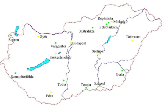
The geographical position of the examined traps are demonstrated in Fig. 5. In this figure green (darker) rings indicate those settlements where the chosen traps can be found.

Figure 5. The regional distribution of the examined light traps

Filtering based on species code

From this point on only those species data were used where there was collection of at least one specimen every year in the examined period (1962-2006), considering all the traps. After filtering, altogether 281 species were left in the database.

After finishing data cleaning and data filtering the Lepidoptera database contained the data of 9 traps, 281 species, which altogether meant 4,020,614 records. The structure of the database is shown in Fig. 6.

EV NAP CSAPDA FAJ DB

Lepidoptera database

.. .

. .

. .

. .

.

Figure 6. The final structure of the Lepidoptera database

The following fields could be found in the database:

EV (year) – year

NAP (day) – the ordinal number of the day within the year CSAPDA (trap) – trap code

FAJ (species) – species code

DB – the number of individuals of the species collected on the given day by the given trap

Merging the trap data

For the sake of decreasing the different abiotic factors and the effects modifying the number of collections happening in different collection places, it is practical to use the data of the greatest possible number of light-tarps (Nowinszky, 2003b). For the creation

of a national time series the data of the traps found in different places had to be merged by species. This is the so called data reducing method (Moon and Kim, 2007), that was carried out by a moving-average calculation. The method of moving-average is suitable for filtering out the extremes occurring in the daily data and to decrease the fluctuations in the data series (Heuvelink and Webster, 2001). This method is also smoothing the time series (Han and Kambel, 2004).

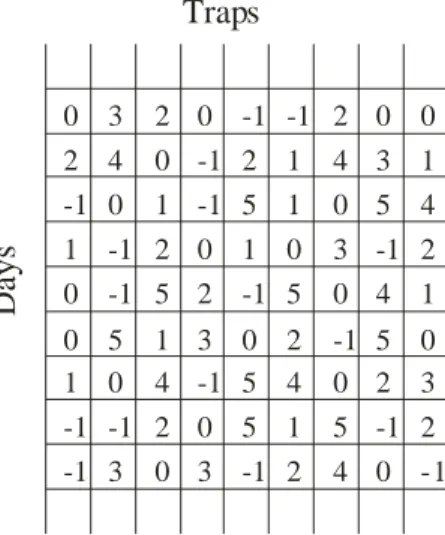
During the moving-average calculations we used the average of 9 days’ (moving- average of 9th grade). We chose number 9, because it corresponded to the number of traps. Fig. 7 demonstrates the window-method that we used to calculate the average, but with fictive data. The figure shows the calculation of the merged data of a given species.

Days can be found in the vertical direction, and traps in the horizontal one. “-1” in a cell indicates that the trap did not operate on the given day. In such case, when calculating the average, the content of the cell is not added to the sum and the value of the divisor is not increased either.

1 0 2 -1 1 0 0

-1 -1

3 4 0 -1 -1 5 0 -1 3

2 0 -1 -1 2 0 0 0

0

0 0 0

0 0

0 0

0 0 -1

-1

-1 -1

-1 -1 -1

-1

-1

1 1

1

1 1

1 1

1 2

2

2 2

2 2 2

2

2 3

3 3

3

3

4

4

4

4 4

4 5

5

5 5

5

5 5

5

Days

Traps

Figure 7. The window used for average calculation

The following formula was used for the calculation of average:

16417 1 ^{8 9} 1

1

, = K

∑ ∑

= =

n k

k

k

i j

j

d

,where:

d

n = the number of cells not containing 1 k = the first day of the window

The maximum value of k is the number of days between 1^st January 1962 and 31^st December 2002, minus 8.

After the calculation of average the data structure outlined in Fig. 8 was presented, where the rows of the table show the years and the ordinal number of the day within the year (16425 rows), and the columns show the species code (281 columns).

Species code

Date

2 3 4 5 6 7

9 79 7

6 5 4 3 2 1 1962 1

2006 365

Figure 8. The Lepidoptera data table after the average calculation

We made a program using Visual Basic language for the creation of the Lepidoptera data warehouse, for the data filtering and for further data processing.

Results

Biological diversity means primarily the diversity of species concerning a given area and a given period of time. For the characterization of diversity we used the number of individuals, the number of species, and the Shannon diversity index.

Time series of aggregate collection

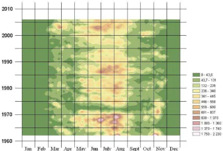
The time series of the number of Lepidoptera collected between 1962 and 2006 is demonstrated in Fig. 9.

Figure 9. The three-dimensional time series figure of the number of individuals based on the Lepidoptera data

It can be seen in the figure that the maximum of the number of individuals occurs in the middle of summer, but there are smaller peaks at the end of March, at the beginning of April and in November, as well.

In summer a significant increase can be observed in the number of individuals, which shows up every 15-20 years.

A remarkable anomaly can be observed in this figure and also in further time series figures in 1972 and 1973. The reason for this is that the definition of Lepidoptera was less accurate in this period.

Number of species (taxon)

One of the most important diversity indices is the number of species (Tóthmérész, 2002), the measure of which depends on the number of entities collected and the attraction zone of the traps. Its drawback is that it does not make a difference between populous species and those that are represented by one or a few entities and moreover, it is territory dependent.

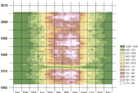
Fig. 10 shows the distribution of the number of collected species. There are fractions in it as well, because the figure was made by interpolation.

Figure 10. The three-dimensional time series figure of the number of species based on the Lepidoptera data

The time series of the number of species shows a smoother picture than that of the number of individuals. However, it can be observed here as well that there are periods (years) when the number of species is significantly higher compared to the neighbouring years.

In the literature Shannon index is used the most commonly for the characterization of diversity, therefore we have also used this for the analysis of our data.

This index is sensitive to the changes of rare species, that is its value decreases with the increase of the number of individuals of dominant species, but it increases with the

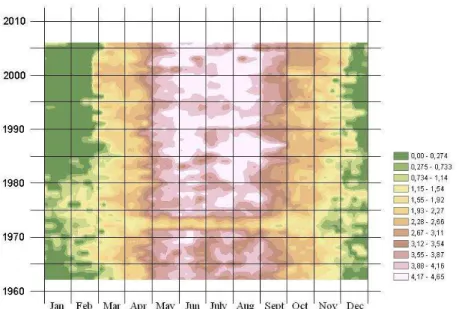
increase of the number of species. The time series of the Shannon index can be seen in Fig. 11.

Figure 11. The three-dimensional time series figure of the Shannon-Wiener index of Lepidoptera data

It can be seen in the figure that the diversity index has maximums in the middle of June and of August. Accordingly, a decrease in diversity can be observed in July.

In the winter period between 1965 and 1980 relatively high diversity values can be seen, in spite of the fact that they cannot be seen either in the time series of the aggregate number of collected individuals (Fig. 9), or in that of the species (Fig. 10).

It is fully visible in all three figures that the values significantly depend on the season.

A significant anomaly can be noticed in 1972 and in 1973 in the time series figures.

A likely reason for this is a personal change at that time, as a consequence of which the definition of Lepidoptera was carried out less precisely.

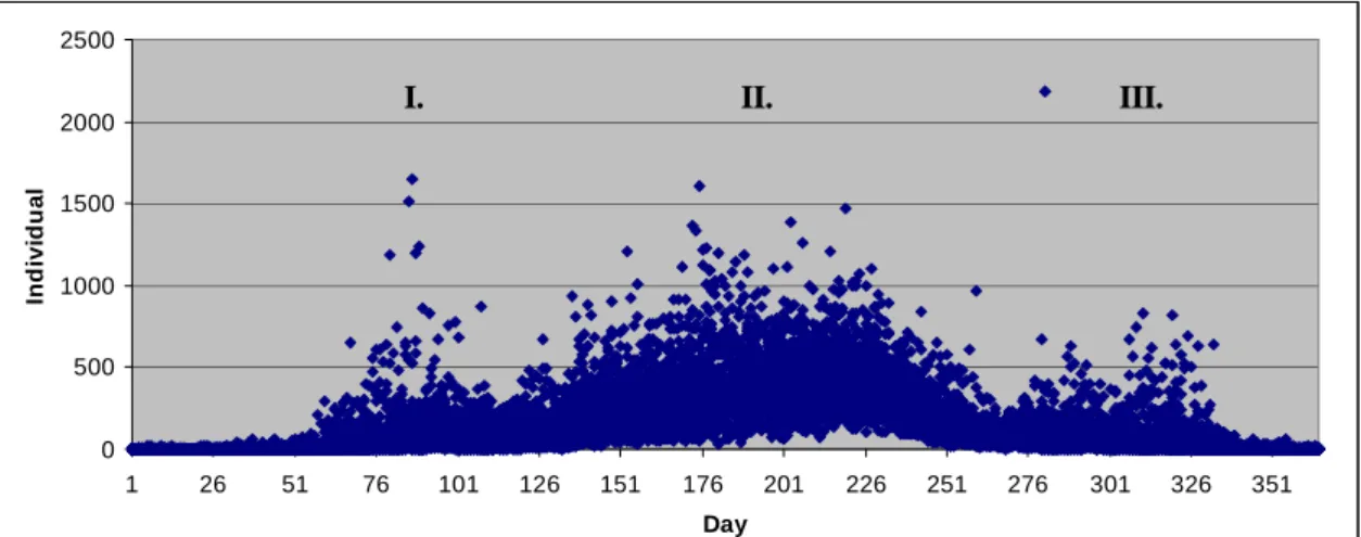
Fig. 12 shows the numbers of individuals collected daily during the 33- year period, Fig. 13 show the dispersion as a function of days.

0 500 1000 1500 2000 2500

1 26 51 76 101 126 151 176 201 226 251 276 301 326 351 Day

Individual

II.

I. III.

Figure 12. The numbers of individuals collected daily based on Lepidoptera data

0 50 100 150 200 250 300 350 400

1 26 51 76 101 126 151 176 201 226 251 276 301 326 351 Day

Dispersion

I. II. III.

Figure 13. Dispersion of the number of individuals collected daily

In Figure 13 three easily separable stages can be seen: the beginning of spring (I.), summer (II.), and late autumn (III.).

The increase in the numbers of individuals are caused by those dominant species that swarm in those periods.

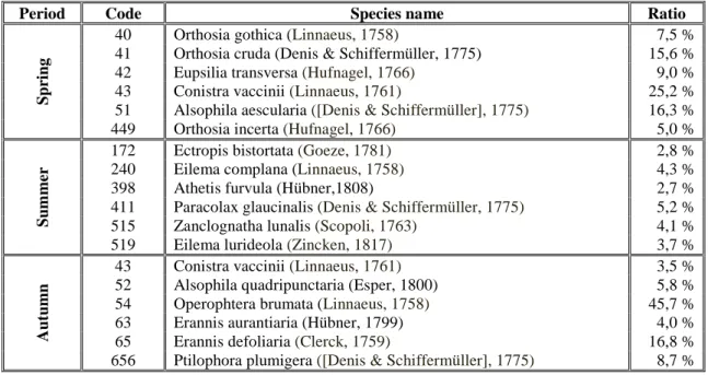
We have made a list of the dominant species of the three periods, which is shown in Table 2. The dominant species appeare in a larger ratio during the spring and the autumn period. The reason for this is that in these periods the number of existing species is lower.

Species 42 and 43 are two-generational. 43 is also dominant in the autumn period, which can be seen in the table. Species 172 has two swarms as well, but both of them are in summer.

Table 2. The ratio of the dominant species in the three periods

Period Code Species name Ratio

40 Orthosia gothica (Linnaeus, 1758) 7,5 %

41 Orthosia cruda (Denis & Schiffermüller, 1775) 15,6 %

42 Eupsilia transversa (Hufnagel, 1766) 9,0 %

43 Conistra vaccinii (Linnaeus, 1761) 25,2 %

51 Alsophila aescularia ([Denis & Schiffermüller], 1775) 16,3 %

Spring

449 Orthosia incerta (Hufnagel, 1766) 5,0 %

172 Ectropis bistortata (Goeze, 1781) 2,8 %

240 Eilema complana (Linnaeus, 1758) 4,3 %

398 Athetis furvula (Hübner,1808) 2,7 %

411 Paracolax glaucinalis (Denis & Schiffermüller, 1775) 5,2 %

515 Zanclognatha lunalis (Scopoli, 1763) 4,1 %

Summer

519 Eilema lurideola (Zincken, 1817) 3,7 %

43 Conistra vaccinii (Linnaeus, 1761) 3,5 %

52 Alsophila quadripunctaria (Esper, 1800) 5,8 %

54 Operophtera brumata (Linnaeus, 1758) 45,7 %

63 Erannis aurantiaria (Hübner, 1799) 4,0 %

65 Erannis defoliaria (Clerck, 1759) 16,8 %

Autumn

656 Ptilophora plumigera ([Denis & Schiffermüller], 1775) 8,7 %

Discussion

In this article the data processing of the National Plant Protection and Forestry Light Trap Network was introduced together with a possible visualization method.

The database created is based on the light trap data. It is suitable for utilization in the most important research areas of the national light trapping. These areas were summarized by Szentkirályi (2002). Among them are faunistical, zoogeographical, taxonomical, phytocenological, ethological, phenological, ecological, etc. examinations (Nowinszky, 2003c).

In case of examinations in swarming phenology the number of generations (Nowinszky, 2003b) and the seasonal changes can be determined by the daily depiction of the entity number of species. This method is widespread both in national and in international publications (Ábrahám and Tóth, 1989; Caldas, 1992; Kimura et al., 2008, Mészáros, 1993; Szentkirályi, 1984).

Investigations in population dynamics provide possibility to draw a conclusion about the tendency of change, based on the data of succeeding years (Nowinszky, 2003b).

This method has also been used by several publications (Conrad et al., 2006; Leskó et al., 1997; Szentkirályi et al.,1995; Szontagh, 2001; Wolda et al., 1998). These publications depict the annual changes and those within a year separately. By merging these two methods we introduced a three-dimensional method that depicts the seasonal and long-term (annual) changes in one figure. The different time series can be depicted much more expressively with this method (Gimesi, 2008, 2009). A similar method was used by Marchiori & Romanowski (2006) to demonstrate insect collecting time series, and also by Mulligan (1998) to demonstrate the seasonal changes of foliages.

In this article we presented the sorting of those Lepidoptera data into databases which were collected by light traps and a visualization method for that. We did not

examine the reasons considering what environmental effects led to certain changes in the time series.

In the future we are willing to perform different investigations with the help of the compiled database. For example: the behaviour of models of species abundance, the behaviour of linear quantile regressions, the regional distribution of different entities and the temporal change of that, and also the different biotic and abiotic effects on population dynamics.

Acknowledgements. We thank deceased Prof. Zsolt Harnos academian for the possibility that the

“Adaptation to Climate Change” Research Group of the Hungarian Academy of Sciences provided a background for finishing our job. We owe Prof. Zoltán Mészáros thanks for his professional help and constructive judgements. We thank the Forestry Scientific Institute and its research workers that they made available for us the Lepidoptera data needed for finishing this essay. Our research was supported by the research proposal OTKA TS 049875 (Hungarian Scientific Research Fund); the VAHAVA project;

the KLIMA-KKT project (National Office for Research and Technology, Ányos Jedlik Programme); the Research Assistant Fellowship Support (Corvinus University of Budapest); the “Bolyai János” Research Fellowship (Hungarian Academy of Sciences, Council of Doctors) and the TÁMOP project 4.2.1/B- 09/1/KMR/-2010-0005.

REFERENCES

[1] Ábrahám, G., Tóth, M. (1989): A káposzta-bagolylepke (Mamestra brassicae L.) rajzásdinamikai vizsgálata szexferomon-, illat- és fénycsapdával. – Növényvédelem 23(3): 119-122.

[2] Arnan, X., Gracia, M., Comas, L., Retana, J. (2009): Forest management conditioning ground ant community structure and composition in temperate conifer forests in the Pyrenees Mountains. – Forest Ecology and Management 258: 51-59.

[3] Balog, A., Marko, V., Adam, L. (2008): Rove beetles (Coleoptera: Staphylinidae) collected during the long term ecological research in a Hungarian oak forest. – Journal of Environmental Biology 29: 263-266.

[4] Bogdanova, G., Georgieva, T. (2008): Using error-correcting dependencies for collaborative filtering. – Data & Knowledge Engineering 66: 402-413.

[5] Böhlen, M. (2003): 3D visual data mining—goals and experiences. – Computational Statistics & Data Analysis 43: 445-469.

[6] Caldas, A. (1992): Mortality of Anaea ryphea (Lepidoptera: Nymphalidae) Immatures in Panama. – Journal of Research on the Lepidoptera 31(3-4): 195-204.

[7] Chefaoui, R.M., Lobo, J.M. (2008): Assessing the effects of pseudo-absences on predictive distribution model performance. – Ecological Modelling 210: 478-486.

[8] Conrad, K.F., Warren, M.S., Fox, R., Parsons, M.S., Woiwod, I.P. (2006): Rapid declines of common, widespread British moths provide evidence of an insect biodiversity crisis. – Biological Conservation 132: 279-291.

[9] Dewar, R.C., Porté, A. (2008): Statistical mechanics unifies different ecological patterns.

– Journal of Theoretical Biology 251: 389-403.

[10] Fan, B. (2009): A hybrid spatial data clustering method for site selection: The data driven approach of GIS mining. – Expert Systems with Applications 36: 3923-3936.

[11] Gimesi, L. (2004). Mesterséges intelligencia alkalmazása a rekultivációban. – Acta Agraria Kaposváriensis 8(3): 1-9.

[12] Gimesi, L. (2008): The use of 3-dimensional graphic display method for presenting the changes in weather. – Applied Ecology And Environmental Research 6(1): 165-176.

[13] Gimesi, L. (2009): Development of a visualization method suitable to present the tendencies of the changes in precipitation. – Journal of Hydrology 377: 185-190.

[14] Gray, J., Chaudhuri, S., Bosworth, A., Layman, A., Reichart. D., Venkatrao, M., Pellow, F., Pirahesh, H. (1997): Data Cube: A Relational Aggregation Operator Generalizing Group-By, Cross-Tab, and Sub-Totals. – Microsoft Corporation, Data Mining and Knowledge Discovery 1: 29-54.

[15] Han, J., Kamber, M. (2004): Adatbányászat – Koncepciók és technikák. – Panem, Budapest.

[16] Heuvelink, G.B.M., Webster, R. (2001): Modelling soil variation: past, present, and future. – Geoderma 100: 269-301.

[17] Hufnagel, L., Sipkay, Cs., Drégely-Kis, Á., Farkas, E., Türei, D., Gergócs, V., Petrányi, G., Baksa, A., Gimesi, L., Eppich, B., Dede, L., Horváth, L. (2008): Klímaváltozás, biodiverzitás és közösségökológiai folyamatok kölcsönhatásai. – In: Harnos, Zs., Csete, L. (ed.): Klímaváltozás: Környezet – Kockázat – Társadalom. Szaktudás Kiadó Ház, Budapest, 229-266.

[18] Ibáňez, J.J., De-Alba, S., Bermúdez, F.F., García-Álvarez, A. (1995): Pedodiversity:

concepts and measures. – Catena 24: 215-232.

[19] Izsák, J. (1994): Applying the jackknife method to significance tests of diagnostic diversity. – Methods of Information in Medicine 33: 214-219.

[20] Izsák, J., Juhász-Nagy, P. (1984): Studies of diversity indices on mortality statistics. – Annales Univ. Sci. Budapestienensis, Sectio Biologica 24-26: 11-27.

[21] Jermy, T. (1961): Kártevő rovarok rajzásának vizsgálata fénycsapdával. – A Növényvédelem Időszerű Kérdései 2: 53-61.

[22] Keim, D.A. (2004): Pixel based visual data miningof geo-spatial data. – Computers &

Graphics 28: 327-344.

[23] Kennedy, R.I., Kee, Y., Van Roy, B., Reed, C.D., Lippman, R.P. (1998): Solving Data Mining Problems Through Pattern Recogntion. – Upper Saddle River, Prentice Hall.

[24] Kevan, P.G. (1999): Pollinators as bioindicators of the state of the environment: species, activity and diversity. Agriculture, Ecosystems and Environment 74: 373-393.

[25] Kimura, G., Inoue, E., Hirabayashi, K. (2008): Seasonal abundance of adult caddisfly (Trichoptera) in the middle reaches of the Shinano River in Central Japan. – 6^th International Conference on Urban Pests, Budapest.

[26] Leskó, K., Szentkirályi, F., Kádár, F. (1997): A gyűrűsszövő (Malacosoma neustria L.) hosszútávú (1962-1996) populációingadozásai Magyarországon. – Erdészeti Kutatások 86-87: 207-220.

[27] Marchiori, M.O., Romanowski, H.P. (2006): Species composition and diel variation of a butterfly taxocene (Lepidoptera, Papilionoidea and Hesperioidea) in a restinga forest at Itapuã State Park, Rio Grande do Sul, Brazil. – Revista Brasileira de Zoologia 23(2): 443- 454.

[28] Menhinick, E.F. (1962): Comparison of invertebrate populations of soil and litter of mowed grasslands in areas treated und untreated with pesticides. – Ecology 43: 556-561.

[29] Mészáros, Z. (1993): Bagolylepkék – Noctuidae. – In: Jermy, T., Balázs, K. (1993): A növényvédelmi állattan kézikönyve 4/B: 453-831.

[30] Mishra, A.K., Özger, M., Singh, V.P. (2009): An entropy-based investigation into the variability of precipitation. – Journal of Hydrology 370: 139-154.

[31] Moon, Y., Kim, J. (2007): Efficient moving average transform-based subsequence matching algorithms in time-series databases. – Information Sciences 177: 5415-5431.

[32] Mulligan, M. (1998): Modelling the geomorphological impact of climatic variability and extreme events in a semi-arid environment. – Geomorphology 24: 59-78.

[33] Nowinszky, L. (2003a): A fénycsapdázás kezdete és jelenlegi helyzete. – In: Nowinszky, L. (ed.) A fénycsapdázás Kézikönyve, Savaria University Press, Szombathely.

[34] Nowinszky, L. (2003b): A fénycsapdás gyűjtési adatok hasznosítása. – In: Nowinszky, L.

(ed.) A fénycsapdázás Kézikönyve, Savaria University Press, Szombathely.

[35] Nowinszky, L. (2003c): A fénycsapdás gyűjtési adatok feldolgozási módszerei. – In:

Nowinszky, L. (ed.) A fénycsapdázás Kézikönyve, Savaria Univ. Press, Szombathely.

[36] Pyle, D. (1999): Data Preparation for Data Mining. – Morgan Kaufmann, San Francisco.

[37] Sipkay, Cs., Hufnagel, L., Gaál, M. (2005): Zoocoenological state of microhabitats and its seasonal dynamics in an aquatic macroinvertebrate assembly (hydrobiological case studes on Lake Balaton, №. 1). – Applied Ecology and Environmental Research 3(2):

107-137.

[38] Skalskia, T., Pośpiech N. (2006): Beetles community structures under different reclamation practices. – European Journal of Soil Biology 42: 316-320.

[39] Szentkirályi, F. (1984): Analysis of light trap catches of green and brown lacewings (Nouropteroidea: Planipennia, Chrysopidae, Hemerobiidae) in Hungary. – SIEEC X.

Budapest, 177-180.

[40] Szentkirályi, F. (2002): Fifty-year-long insect survey in Hungary: T. Jermy’s constributions to light trapping. – Acta Zoologica Academiae Scientiarum Hungaricae 48(1): 85-105.

[41] Szentkirályi, F., Szalay, K., Kádár, F. (1995): Jeleznek-e klímaváltozást a fénycsapdás rovargyűjtések? – Erdő és Klíma Konferencia, Noszvaj 1994: 171-177.

[42] Szontagh, P. (1975): A fénycsapda hálózat szerepe az erdészeti kártevők prognózisában.

– Növényvédelem 11: 54-57.

[43] Szontagh, P. (2001): Rovarok okozta problémák és kihívások erdeinkben. – Erdészeti Tudományos Intézet Kiadványai 15: 35-37.

[44] Tóthmérész, B. (1997): Diverzitási rendezések. – Scientia, Budapest

[45] Tóthmérész, B. (2001): Kvantitatív ökológiai kutatások különös tekintettel a skálázási és mintázati problémákra. – In: Borhidi, A. (2001): Ökológia az ezredfordulón, Budapest, Akadémiai Kiadó, 15-25.

[46] Tóthmérész, B. (2002): A diverzitás jellemzésére szolgáló módszerek evolúciója. – In:

Salamon-Albert, É. (2002): Magyar botanikai kutatások az ezredfordulón.

[47] Wolda, H., O'Brien, C.W., Stockwell, H.P. (1998): Weevil Diversity and Seasonally in Tropical Panama as Deduced from Light trap Catches (Coleoptera: Curculionoidea). – Smithsonian Institution Press, Washington, D.C.