THE EFFECT OF CLIMATE CHANGE ON THE POPULATION OF SYCAMORE LACE BUG (CORYTHUCA CILIATA, SAY, TINGIDAE HETEROPTERA) BASED ON A SIMULATION
MODEL WITH PHENOLOGICAL RESPONSE
M.LADÁNYI*–L.HUFNAGEL
Corvinus University of Budapest, Department of Mathematics and Informatics H-1118 Budapest, Villányi út 29-43., Hungary
(phone: +36-1-482-6261; fax: +36-1-466-9273)
*e-mail: marta.ladanyi@uni-corvinus.hu
(Received 10th Sep 2005, accepted 10th Oct 2006)
Abstract. Climate change affects on insect populations in many ways: it can cause a shift in geographical spread, abundance, or diversity, it can change the location, the timing and the magnitude of outbreaks of pests and it can define the phenological or even the genetic properties of the species. Long-time investigations of special insect populations, simulation models and scenario studies give us very important information about the response of the insects far away and near to our century. Getting to know the potential responses of insect populations to climate change makes us possible to evaluate the adaptation of pest management alternatives as well as to formulate our future management policy. In this paper we apply two simple models, in order to introduce a complex case study for a Sycamore lace bug population. We test how the model works in case the whether conditions are very different from those in our days. Thus, besides we can understand the processes that happen in present, we can analyze the effects of a possible climate change, as well.
Keywords: climate change, insects, pest management, simulation, agriculture
Introduction and Aims
Simulation is the ultimate tool for forecasting the effect of climate and other environmental factors on the ecosystem, since the real circumstances of future cannot be examined empirically. However, it may take several years to reach the stage when these forecasts will be usable in the agriculture since the longer climate forecasts are not yet good enough [18], [15], [39]. There have been made several projects in Hungary with simulation model applications and with valuable results about the effects of climate change on the yield of arable crops [16], [17], [29], [27], [30], [31], [32], but there are very rare references on plant – pest populations.
In our paper we refer to one of our earlier population dynamical food web biomass model together with a phenology model based on the food web model [33], [34]. In the food web model the seasonal weather aspects, the nutrient content of soil and the biotic interactions are considered. To simulate the interactions, a discrete difference equation system was used. The general equation of the model is based on three terms: the first one is to express the activity of the individual depending on the temperature, the second one is to describe the effect of the quality and the quantity of the nutrient of the populations and the third one is to display the effect of the predators.
Besides quantitative (biomass) changes, however, there are also seasonal qualitative changes during the evolution of the entities. These changes are described by phenology.
It is obvious to ask, how the number of entities can be derived from a given amount of biomass. More exactly, if the phenological phases of the population, together with their biological properties, are known, how can one define the number of the entities of each phenophase at a given point of time? Our phenology model is to solve this problem.
In what follows, we apply the above two models in a drastically simplified form, in order to introduce a complex case study for a Sycamore lace bug (Corythuca ciliata) population.
In addition to the foregoing, we found it very useful to ask, how the model works in case the whether conditions are very different from those in our days. Thus, besides we can understand the processes that happen in present, we can analyze the effects of a possible climate change, as well.
Sycamore lace bug can be an excellent indicator for the climate researchers as it has much less biotic interactions comparing with other native species or with species having native host. Sycamore lace bug has other advantages, too, namely, that it is monophagous in Europe and it can quite easily be monitored, due to its way of life [55], [44].
Obviously, our contemporary knowledge does not make us possible to predict the future, even for the quite well known Corythuca ciliata - Sycamore tree (Platanus hybrida) populations. A reasonable aim can be, however, to find out, what is predicted by our model for simulated weather data with different parameters for different assumptions. This aim corresponds to the aims of VAHAVA project of the Hungarian Academy of Sciences, as well as to those of international climate change projects [4, 5, 20, 21, 35, 54].
To explore the possible effects of an unknown climate change in future, we need not real but realistic alternative climate scenarios. First, we define the concept of climate scenario.
Climate scenarios are possible future climates in a set. Each of them is made consistently by applying scientific principles; however any of them has a fixed (calculable) possibility. A climate scenario is one of the possible climates and it is by no means a prediction [3, 21].
After having recognized the ecological consequences of climate change, together with UNEP, WMO (World Meteorological Organization) has established IPCC (Intergovernmental Panel on Climate Change) with the task of giving unbiased and detailed information about climate change and its expected effects.
During our research, we applied the principles defined by IPCC and we used some of the most commonly accepted scenarios presented in international reports. The most serious scenarios, themselves, are results of simulation models. For generating scenarios the so-called GCMs are generally used (General Circulation Model or Global Climate Model). GCMs have been successfully used to estimate the climate change on arable crops yield in Hungary in a 15- and a 30-year scenario [26].
In our research we applied six different scenarios, such as:
•-Scenario BASE is a simulated weather data series with the same conditions as we have at present.
• Scenarios GFDL2535 and GFDL5564 have been created by Geophysical Fluid Dynamics Laboratory (U.S.A.) with the assumption that CO2 concentration doubles in atmosphere. The difference between the scenarios is their resolution level. (The later has higher resolution.)
• Three very different scenarios have been worked out by United Kingdom Meteorological Office (UKMO), namely UKHI (high-resolution equilibrium climate change experiment), UKLO (low-resolution equilibrium climate change experiment) and UKTR (high-resolution transient climate change experiment). The first two scenarios of UKMO (UKHI, UKLO) are so-called equilibrium models, that is to say, assumed that CO2-concentration doubles in atmosphere, GCM runs until an equilibrium state with stable surface temperature. The third scenario of UKMO (UKTR) is a transient model that describes the gradually changing climate assuming a gradually increasing CO2
content of atmosphere [4, 24].
Note that the results of GCMs should be scaled on the examined region with the help of empirical statistical methods [5]. In our paper, we present the results of the 15th year of each 30-year period scenario concerning the years around 2050. The scaling of the scenarios for the region of Hungary was made in the frame of CLIVARA project (Climate Change, Climatic Variability and Agriculture in Europe). The database and the references were made available for us by professor Zs. Harnos, the Hungarian leader of the project.
To sum it up, in this paper we followed two main aims:
• To create a complex population dynamical model with phenology responses for Sycamore lace bug based on an earlier field-work [44].
• To introduce a case study for the above model applied for some widely accepted climate-change scenarios.
Review of literature
In our century increasing societal, environmental, and economic pressures force us to develop new agricultural pest management strategies. Interdisciplinary approaches have the aim to find the way, how the environmental degradation caused by the use of chemicals can be decreased, how the productivity can be increased by reducing insect and disease damage to cultivated plants, and how the competition with weeds can be reduced. Crop and forestry population system models are useful tools to examine the interrelationships among plants, pests and the environment. With simulation models we can find optimal strategies that meet individual and societal goals.
Improved techniques for managing pests require weather and insect data from thoroughly maintained monitoring as well as climate information and forecast to determine their suitability. Climatic change, including global warming and increased variability require improved analyses that can be used to assess the risk of the existing and the newly developed pest management strategies and techniques, and to define the impact of these techniques on environment, productivity and profitability. Each technique has to be evaluated whether and how it is suitable in the farming system where they are to be applied.
Nowadays, several studies are investigating the impact of climatic change on insect populations. Some of the effects can be discovered in laboratories, only (e.g. the effect of humidity [6]), some of them need field observations maintenance. The impact of climate change, moreover, alters from region to region, from species to species. Quite a lot of new methods from different disciplines are used to detect the most important
effects. Therefore, the studies of climate change effects are considering different aspects, such as palaeontological, agricultural, medical, geological, biological as well as the aspects of forestry management. This widespread research work requires interdisciplinary cooperation of researchers from several fields [53]. We give a short review of the main approaches.
The aspect of palaeontology
One of the most important ways to find out what climate change can bring us is to look back into the very past. A few thousand years ago some regions were characterized by such kind of vegetations that existed within warming thermal conditions analogous to those today. For example, the transition from parkland vegetation and insects to the one of coniferous forest of south-western Ontario region indicates that the climate continued gradually warm through the mid-Holocene [48].
The Lateglacial-Holocen transition is characterized by major changes in the insect fauna, too, reflecting an extremely rapid climate change in South-Sweden, as well as in Swiss-Alps. In these regions the cold-adapted species assemblage was immediately replaced by temperate species [36], [37]. During the same time period most of temperate species of Chihuahuan Desert (Texas) were replaced either by desert species or more cosmopolitan taxa [12]. The above studies pointed out the dependency of the changes in climate and fauna. The question of how these kinds of responses proceed was studied by Amman [1].
The approaches with models, simulations and scenarios
Developing ecological and simulation models is a very useful tool to find out the response of a system to an event or a series of events. Ecological or meteorological models describe biological or climate properties mathematically, while simulations make a computer based models system supplied with a great amount of empirical data.
To reach his above mentioned palaeontological results in Swiss-Alps, Lemdahl [37]
applied a so-called climatic reconstruction (MCR) method that simulates realistic climate data in the past. Simulated weather data, however, are most commonly used to examine the potential future effects. These approaches are called scenario studies.
The main problems that have to precede scenario studies are, nevertheless, the evaluation, the validation and verification of the applied models. Though several models have been developed e.g. for the carbon budget of boreal forests, enormous problems remain in incorporating pest effects in these models. These problems have their origins, partly in scaling. The common problems of verification and validation of model results are particularly troublesome in projecting future productivity [56].
A main point of scenario studies is, therefore, how the applied model should be scaled. Hanson [19] noticed that although early model predictions of climate change impacts suggested extensive forest dieback and species migration, more recent analyses suggest that catastrophic dieback will be a local phenomenon, and changes in forest composition will be a relatively gradual process. Better climate predictions at regional scales, with a higher temporal resolution (months to days), coupled with carefully designed, field-based experiments that incorporate multiple driving variables (e.g.
temperature and CO2); will advance our ability to predict the response to climate change.
Time-dependent models developed at fine spatial resolution of experimental studies are widely used to forecast how plant - insect populations will react over large spatial
extents. Usually the best data available for constructing such models comes from intensive, detailed field studies. Models are then scaled-up to coarser resolution for management decision-making. Scaling-up, however, can affect model predictions and dynamical behaviour which can result misinterpretation of model output. The potential negative consequences of scaling-up deserve consideration whenever data measured at different spatial resolutions are integrated during model development, as often happens in climate change research [13].
Chen [7] investigates the integrated effects of insect infections, management practices, carbon cycle and climatic factors both at regional and global scales.
To see that there can be great difference between the responses of even similar species, we refer to Conrad et al [8]. They examined the garden tiger moth (Arctia caja) that was widespread and common in the UK in the last century, but its abundance fell rapidly and suddenly after 1984. The most UK butterflies are expected to increase under UK climate change scenarios of global warming. Contrary to them, garden tiger is predicted to decrease further because of warm wet winters and springs, to which it is very sensitive [38].
Ecological models serving climate change studies
We give a short list of the most widely applied ecological models focused to insect populations.
The Forest Vegetation Simulator (FVS) is a distance-independent, geographic region dependent individual-tree forest growth model that has been widely used in the United States for about 30 years to support management decision making. It has been continuously extended, improved and adapted to further management tasks like prediction of climate change effects. Component models predict the growth and mortality of individual trees, and extensions to the base model represent disturbance agents including insects, pathogens, and fire. The geographic regions are represented by regionally specific model variants. The differences are due to data availability and the applicability of existing models. The model supports specification of management rules in the input [10], [11].
The Phenology and PopulatIoN SIM (INSIM) is an age - structured model that needs biological information on the insect species and gives calculations on the number of individuals and the development of the population. It involves a complex pest – natural enemies model, as well [41], [42].
Agro – ECOsystem ManagemenT and OPtimization Model (ECOTOPE) is a typical simulation model, which describes processes of an agricultural ecosystem for crop growth, nitrogen dynamics in soil and pest population. It is used to derive optimum management strategies [49], [50], [51].
Boundary LAYER Model (BLAYER) simulates atmospheric flows and it has been adapted to forecast the timing and location of insect pest migrations into the United States corn belt. It is very useful to study the possible changes in pest populations like migration or dispersal patterns resulted by climate change [45].
Boll Weevil DISPersal Model (BWDISP) is a stochastic simulation model that predicts the spread of boll weevil populations on cotton. Because the development and dispersal of this insect is sensitive to temperature, it is important to understand how this insect will potentially respond to climate change. In addition, without proper management of this pest, other secondary pests may attack the crop [40].
Northern Corn ROOTWORM Model (ROOTWORM) is a process – oriented simulation model that examines the population dynamics of corn – rootworm in the northern United States. The rootworm attacks both the roots and tassels of corn, decreasing yields. The model examines how planting date affects the population dynamics of the insects. It gives information on phenology and the number of individuals in each growth state of corn. The model can analyze global change impact on the population levels and distribution of the insects, as well as the potential economic impacts [43].
The potential responses of insects to climate change
Climate and weather can substantially influence the development and distribution of insects. Current estimates of changes in climate indicate an increase in global mean annual temperatures of 1°C by 2025 and 3°C by the end of the next century. Such increases in temperature have a number of implications for temperature-dependent insects, especially in the region of Middle - Europe. Changes in climate may result changes in geographical distribution, increased overwintering, changes in population growth rates, increases in the number of generations, extension of the development season, changes in crop-pest synchrony of phenology, changes in interspecific interactions and increased risk of invasion by migrant pests.
Under the climatic changes projected by the Goddard Institute for Space Studies general circulation model, northward shifts in the potential distribution of the European corn borer of up to 1220 km are estimated to occur, with an additional generation found in nearly all regions where it is currently known to occur [46].
Several results on the effect of climate change on insects were published in the field of forestry sciences, since insects cause considerable loss of wood that has an adverse effect on the balance of carbon sequestered by forests. Volney and Fleming [56] state that pests are major, but consistently overlooked forest ecosystem components that have manifold consequences to the structure and functions of future forests. Global change will have demonstrable changes in the frequency and intensity of pest outbreaks, particularly at the margins of host ranges.
Ayres and Lombardero [2] have shown that climate change has
• direct effects on the development and survival of herbivores and pathogens;
• physiological changes in tree defenses; and
• indirect effects from changes in the abundance of natural enemies (e.g.
parasitoids of insect herbivores), mutualists (e.g. insect vectors of tree pathogens), and competitors.
Because of the short life cycles of insects, mobility, reproductive potential, and physiological sensitivity to temperature, even modest climate change will have rapid impacts on the distribution and abundance of many kinds of insects. To consider scenario studies, some of them predict negative, but many forecast positive effects on insects. E.g. global warming accelerates insect development rate and facilitate range expansions of pests, moreover, climate change tends to increase the vulnerability of plants to herbivores. One alarming scenario is that climate warming may increase insect outbreaks in boreal forests, which would tend to increase forest fires and exacerbate further climate warming by releasing carbon stores from boreal ecosystems [2].
Hanson and Weltzin [19] studied especially the drought disturbances caused by climate change. They showed that severe or prolonged drought may render trees more susceptible to insects.
Climate variability at decadal scales influences the timing and severity of insect outbreaks that may alter species distributions. Coops and al. [9] have presented a spatial modelling technique to infer how a sustained change in climate might alter the geographic distribution of the species. Using simulations they produced a series of maps that display predicted shifts of zones where the species they examined might expand its range if modelled climatic conditions at annual and decadal intervals were sustained.
The connection between temperature tolerance and phenology of insects was investigated by Klok and Chown [25]. They defined how current climate change like increased temperature and decreased rainfall affect on physiological regulation and susceptibility.
Powell and Logan [47] have reviewed the mathematical relationship between environmental temperatures and developmental timing and analyzed circle maps from yearly oviposition dates and temperatures to oviposition dates for subsequent generations. Applying scenarios for global warming they proved that adaptive seasonality may break down with little warning with constantly increasing (and also decreasing) temperature.
Forecasted increases in atmospheric CO2 and global mean temperature are likely to influence insect – plant interactions. Plant traits important to insect herbivores, such as nitrogen content, may be directly affected by elevated CO2 and temperature, while insect herbivores are likely to be directly affected only by temperature. Flynn et al. [14]
stated that insect populations did not change significantly under elevated CO2, but tended to increase slightly. Average weight decreased at high temperatures. Plant height and biomass were not significantly affected by the CO2 treatment, but growth rates before infestation were enhanced by elevated CO2. These results indicate that the combined effects of both elevated CO2 and temperature may exacerbate pest damage to certain plants, particularly to plants which respond weakly to increases in atmospheric CO2.
Up to this time, as we have seen, mainly two climatic factors – temperature and humidity have been investigated. Though, it is possible that some parts of solar radiation have at least the same importance in controlling insect populations [6].
Last, but not least, changes in climate increases the likelihood of insect transport from regions to regions, as well [22, 23, 55, 57].
The special agricultural aspects of climate change effect on insects
Global climate change impact on plant - pest populations depends on the combined effects of climate (temperature, precipitation, humidity) and other components like soil moisture, atmospheric CO2 and tropospheric ozone (O3). Changes in agricultural productivity can be the result of direct effects of these factors at the plant level, or indirect effects at the system level, for instance, through shifts in insect pest occurrence.
With respect to crops, the data suggest that elevated CO2 may have many positive effects, including yield stimulation, improved resource - use efficiency, more successful competition with weeds, reduced O3-toxicity, and in some cases better pest and disease resistance. However, many of these beneficial effects may be lost - at least to some extent - in a warmer climate. Warming accelerates plant development and reduces grain-fill, reduces nutrient-use efficiency, increases crop water consumption, and favours weeds over crops. Also, the rate of development of insects may be increased. A major effect of climate warming in the temperate zone could be a change in winter survival of insect pests, whereas at more northern latitudes shifts in phenology in terms
of growth and reproduction, may be of special importance. However, climate warming disturbs the synchrony between temperature and photoperiod; because insect and host plant species show individualistic responses to temperature, CO2 and photoperiod, it is expected that climate change will affect the temporal and spatial association between species interacting at different trophic levels. Although predictions are difficult, it seems reasonable to assume that agro - ecosystem responses will be dominated by those caused directly or indirectly by shifts in climate, associated with altered weather patterns, and not by elevated CO2 per se. Overall, intensive agriculture may have the potential to adapt to changing conditions, in contrast to extensive agricultural systems or low - input systems which may be affected more seriously [18].
Crop protection in Europe became strongly chemically oriented in the middle of the last century. An excellent climate for fast reproduction of pests and diseases demanded high spray frequencies and, thus, resulted in quick development of resistance against pesticides. This initiated a search for alternatives of chemical pesticides, like natural enemies for control of pests. A change from chemical control to very advanced integrated pest management programs (IPM) in European greenhouses took place at the end of the last century [38]. For the main greenhouse vegetable crops in northern Europe, most insect problems can now be solved without the use of insecticides. IPM without conventional chemical pesticides is a goal that will be realized for most of the important vegetables in Europe, not limited to greenhouse vegetables. At the same time, however, climate change affects the distribution, the phenology, the susceptibility and the interrelationship of insects drastically, which emphasize the risk of sustainable crop protection by loosing the control on pests - natural enemies’ populations.
Materials and Methods The methods of modelling
In a former work [33] we have introduced a food web population dynamical model that describes the biomass change of the members of a food web with a cultivated plant and two kinds of weed, monophagous and polyphagous pests and a predator. In what follows, we apply this model for our Corythuca ciliata – Sycamore tree population with three purposes:
• we show, how the model works in practise
• we find out the model-parameters for a Corythuca ciliata – Sycamore tree population and
• with the help of the food web population dynamical model, we try to get information out of weather parameters for plant protection purposes.
The examined Corythuca ciliata – Sycamore tree population shows a very simple case of the general food web seasonal population dynamical model:
• Though there exist several natural enemies of Sycamore lace bug, under natural circumstances they do not appear at all in Hungary, or they are playing no limiting role in reproduction. Thus, we consider Sycamore lace bug in the model, as a pest of Sycamore tree having no predator.
• Though the rate of Sycamore lace bug infection can be quite high in Hungary, the size of the population has never been limited by the Sycamore tree population. Thus, we assume in the model, that there is no nutrient limitation of Sycamore lace bug.
• Sycamore lace bug is monophagous and nowadays it is the most important pest of Sycamore trees.
To simulate the population of Sycamore lace bug, we used a model with discrete- time (with daily scale), deterministic and weather-dependent difference equations.
The model has a format of MS Excel so that it can widely be applied. The parameters of the model were fitted to the empirical data with the help of MS Excel Solver. The empirical data were gathered between 1989 and 1999 in public parks of Budapest, Hungary [44].
Results
General biomass model
Our drastically simplified food web biomass seasonal population dynamical model applied for the examined Corythuca ciliata – Sycamore tree population is generally as follows:
t t
t M R
M +1 = ⋅ where
the amounts of the biomass of Sycamore lace bug population at the (t+1)th and at the tth points of time are denoted by Mt+1 and Mt, respectively
the activity term of the entities of M is denoted by Rt is depending on the daily average temperature T.
In what follows the terms of the general equation are introduced.
The activity term Rt and the cumulated activity tPh
t
t R
cum
≥s
Activity term Rt expresses that the agro-ecological process – that was represented by the general biomass model above – is depending on the daily average temperature;
nevertheless, the effect of the same temperature on the entities can be different in different phenological phases (Table 1 and 2).
Let us denote by ts the so-called ‘first spring day of the population’ and by tw the
‘first winter day of it’. We say, that the vegetation period of a population lies between ts and tw.
The cumulated activity is defined by
≥
⋅
<
=
∑
=
≥ s
Ph i t
t i
Ph i
s Ph
t t
t R SW t t
t t R
cum
s
s if
if 0
Cumulated activity tPh
t
t R
cum
≥s cumulates the values of activity terms Rt of Sycamore lace bug from a starting point of time, ts (from ‘the first spring day of Sycamore lace bug’), in the case phase Ph holds. Ph denotes one of Lij (for the jth larva state of the ith generation, i=1, 2, j=1, 2, ... ,5) and Ii (for the imago state of the ith generation i=1, 2, 3).
Cumulated activity tPh
t
t R
cum
≥s of Sycamore lace bug is calculated with the help of a characteristic function SWtPh:
( )
( )
{ }
[ ] ( )
11
1
0 if if
0 if 1
1 , 0 , max
min 1 0
1 t and Ph I
I Ph
I Ph and t
SW T
CumR SW SW
Ph Ph
Ph t Ph
m Ph t Ph t I
Ph Ph t
>
>
=
>
=
−
−
−
=
∏
∏
>
>
where
mPh
T denotes the minimum of cumulated activity of Sycamore lace bug tPh
t
t R
cum
≥s that is necessary to enter phase Ph
and relation Ph> Ph means that „for all phases later than phase Ph ”.
For a fixed point of time t and a phenophase Ph, SWtPh shows, whether the phase Ph holds at a point of time t, that is to say:
hold not does if
holds if
1 0
Ph SWtPh Ph
=
(Figures 1, 2, 3 and 4)
Table 1. The values of activity term Rt of the daily average temperature T. Activity term expresses that the agro-ecological process Mt+1 =Mt⋅Rt is depending on the daily average temperature differently in different phenophases.
Conditions Rt Earlier than the first spring day t <ts 0.90
33 22< tI−31 <
t R
cum 0.90
In the third Imago phase
33
3
1 >
− I t Rt
cum 1
<5
T 0.98
10
5≤T < 0.99
15
10≤T < 1.06
21
15≤T < 1.08
26
21≤T < 1.04
Else
≤T
26 0.80
cumR
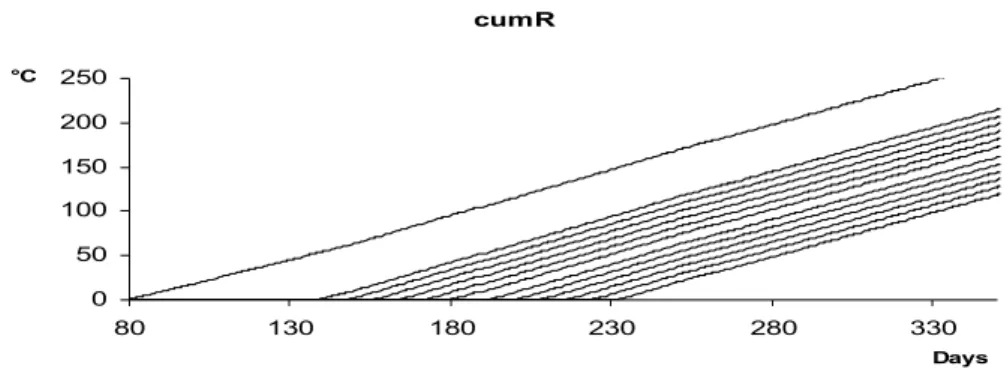
0 50 100 150 200 250
80 130 180 230 280 330
Days
°C
Figure 1. The graphs of cumulated activities tPh
t
t R
cum
M
≥s, for Ph = I1, L11, L12 , L13,, L14,, L15 as well as for Ph = I2, L21, L22 , L23 , L24 , L25, I3.. tPh
t
t R
cum
≥s cumulates the values of activity terms Rt of Sycamore lace bug from a starting point of time, ts.
Note that though the graphs of tPh
t
t R
cum
M
≥s, seem to be straight lines, it is not the fact.
cumR_magnified_1
150 160 170 180 190 200
Days
cumR_magnified_2
180 182 184 186 188 190
Days
Figure 2. The graphs of cumulated activities tPh
t
t R
cum
M
≥s, seem to be straight lines, it is not the fact. Their lines brake several times.
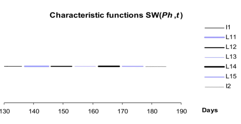
First, we assume that the phenophases of the population are disjunctive, that is to say each entity of the population belongs to an only phase Ph. (Later we omit this condition.) Function SWtPh equals to 1 if and only if the Sycamore lace bug population has more than zero number of entities in phase Ph at a given point of time t, and equals to 0, else. The change of the values of function SWtPh
• from 0 to 1 is caused by the fact cumulated activity tPh
t
t R
cum
≥s has reached the minimum that is necessary for the entities to enter phase Ph +1, that is to say
Ph m Ph t t
t R T
cum
s
≥ > .
• from 1 to 0 is caused by the fact the next phase has been entered.
Characteristic functions SW(Ph,t)
130 140 150 160 170 180 190 Days
I1 L11 L12 L13 L14 L15 I2
Figure 3. The graphs of characteristic functions SWtPh for Ph = I1, L11, L12, L13, L14, L15, and I2
Characteristic functions SW(Ph,t)
180 190 200 210 220 230 240 Days
I2 L21 L22 L23 L24 L25 I3
Figure 4. The graphs of characteristic functions SWtPh for Ph = I2, L21, L22, L23, L24, L25, and I3
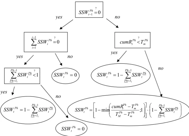
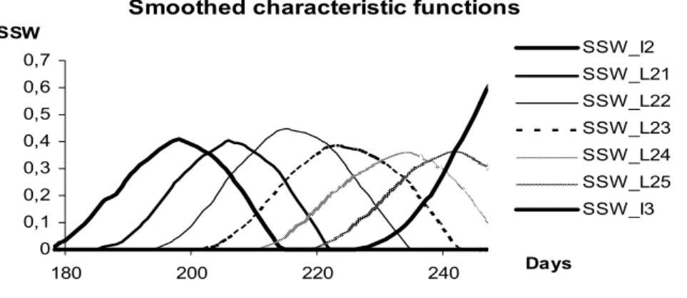
The smoothed characteristic function SSWtPh
Our main aim is to define the current number of the entities if we know the current biomass of Sycamore lace bug. On the way to our goal we have to keep in mind that there is a point of time a phase is entered first, and there is another one at which the process of metamorphosis is finished for the whole population. This means that there can usually appear more than one phenological phases at the same time (as opposed to our earlier assumption). Thus, function SWtPh that ’switches’ on/off the phases has to be ‘smoothed’ in order to get the number of entities later more exactly. The smoothed characteristic function SSWtPh is defined as follows:
At t=0, we have SSWtI1 =1 and SSWtPh =0 for all phases Ph>I1. (At the beginning of spring there are entities in the first Imago phase, only.) At the point of time the minimal value of cumulated activity tPh−1
t R
cum , that is necessary to enter phase Ph (denoted by TmPh−1, see Table 2), has been exceeded ( tPh−1
t R
cum >TmPh−1), the entities of phase Ph – 1 are starting to enter phase Ph. (We say, that at the point of time t, when
−1 Ph t Rt
cum >TmPh−1 first, phase Ph is entered first.) During the time of metamorphosis
from Ph – 1 to Ph, the value of SSWtPh is growing from zero to 1 (though, it is not necessary that SSWtPh reaches 1, indeed. We can say only that 0≤SSWtPh ≤1). The value of SSWtPh reaches its potential maximum (potmaxSSWtPh =1), if
−1 Ph t Rt
cum >TMPh−1 and if tPh
t R
cum <TmPh, that is to say, the metamorphosis to the next phase, Ph + 1 has still not began. (At this point of time the process of metamorphosis from Ph – 1 to Ph is finished for the whole population.) In the case the minimal value of cumulated activity tPh
t R
cum , that is necessary to enter phase Ph + 1 (denoted by TmPh), has been exceeded ( tPh
t R
cum >TmPh), then SSWtPh starts to decrease monotonously to zero.
?0
1 =
−Ph
SSWt
?0
1
1
∑
− == t
i
Ph
SSWi cumRtPh<?TmPh
?1
1
1
∑
− <= Ph
I Ph
Ph
SSWt SSWtPh =0
∑
−=
−
= 1
1
1 Ph
I Ph
Ph t Ph
t SSW
SSW
∑
−=
−
= 1
1
1 Ph
I Ph
Ph t Ph
t SSW
SSW
−
⋅
−
− −
=
∑
−= 1
1
1 1
; min
1 Ph
I Ph
Ph Ph t
m Ph M
Ph m Ph Ph t
t SSW
T T
T SSW cumR
SSWtPh =0
Figure 5. The way of evaluation of function SSWtPh. Considering that the metamorphosis from phase Ph to phase Ph + 1 is a continuous process, characteristic function SWtPh that ’switches’
on/off the phases has to be smoothed in order to get the number of entities later more exactly.
(For Ph=I1 we say that SSWtPh−1 =0 for each t.) If tPh
t R
cum > TmPh at the point of time t when tPh−1
t R
cum >TMPh−1 first, then SSWtPh cannot reach its potential maximum value (maxSSWtPh < potmaxSSWtPh =1), because the metamorphosis from Ph - 1 to Ph ends later than the metamorphosis from Ph to Ph + 1 starts.
yes
no yes
yes
no yes
no
no
At the point of time at which the whole process of metamorphosis from Ph to Ph + 1 is finished, namely, when tPh
t R
cum >TMPh, the value of SSWtPh becomes to be equal to, and keeps to be, zero (Figures 5, 6 and 7).
It is easy to see that
∑
=Ph Ph
SSWt phases all for
1.
Table 2. The values of TmPh and TMPh. At the point of time t, when tPh−1
t R
cum >TmPh−1 first, phase Ph is entered first. At the point of time tPh−1
t R
cum >TMPh−1 first, the process of metamorphosis from Ph – 1 to Ph is finished.
Phase I1 L11 L12 L13 L14 L15 I2 L21 L22 L23 L24 L25
Ph
Tm 52 7 7 7 7 7 7 7 7 7 7 7
MPh
T 67 27 32 37 37 37 37 37 42 42 42 42
Smoothed characteristic functions
0 0,1 0,2 0,3 0,4 0,5 0,6 0,7
140 160 180 200 Days
SSW SSW_I1
SSW_L11 SSW_L12 SSW_L13 SSW_L14 SSW_L15 SSW_I2
Figure 6. The graphs of smoothed characteristic functions SSWtPh for Ph = I1, L11, L12, L13, L14, L15, and I2
Smoothed characteristic functions
0 0,1 0,2 0,3 0,4 0,5 0,6 0,7
180 200 220 240 Days
SSW SSW_I2
SSW_L21 SSW_L22 SSW_L23 SSW_L24 SSW_L25 SSW_I3
Figure 7. The graphs of smoothed characteristic functions SSWtPh for Ph =I2, L21, L22, L23, L24, L25, and I3
The number of entities of Sycamore lace bug (NoItPh)
Finally, the numbers of entities of Sycamore lace bug in all phenophases will be calculated as follows. Set out from an estimated value of the number of entities of phase
I1 at the point of time t0 =0:
1
1 0
0 I
I
m NoI = M
where mI1 denotes the average mass of an only entity of Sycamore lace bug in phenophase I1.
The number of entities of Sycamore lace bug for a phenophase Ph) at a point of time
>0
t is obtained as:
{ }
=
=
⋅
=
≠
⋅ ⋅
=
−
−
−
− ∈
) 2 , 1 (
) 2 , 1 ( max
, min
1 1
1 1
1 1
i L Ph if m SSW
M
i L Ph if NoI
k m SSW
M NoI
i Ph
Ph t t
t
i Ph
Ph t t Ph Ph
Ph t t
t Ph
t
where mtPh denotes the current average mass of an only entity of Sycamore lace bug in the phenophase Ph at a point of time t:
Ph t t Ph
t NoI
m = M
{
−1}
∈ Ph
t means: “for all t for which SSWtPh−1 >0”,
and the multiplier term kPh expresses the standard mortality during the metamorphosis from phase Ph−1 to phase Ph (See Figures 8 and 9).
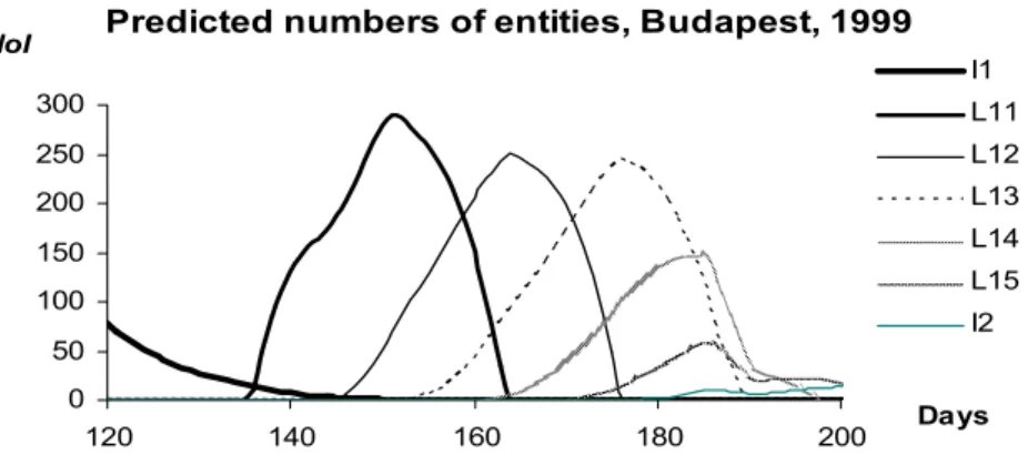
Predicted numbers of entities, Budapest, 1999
0 50 100 150 200 250 300
120 140 160 180 200 Days
NoI I1
L11 L12 L13 L14 L15 I2
Figure 8. The numbers of Sycamore lace bug entities NoItPh in Budapest, between the 120th and 200th days of year 1999, predicted by the model for Ph = I1, L11, L12, L13, L14, L15 and I2
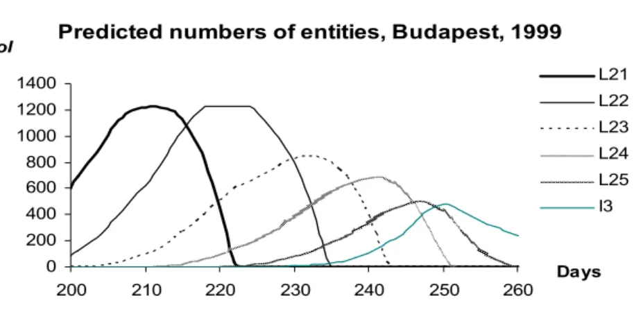
Predicted numbers of entities, Budapest, 1999
0 200 400 600 800 1000 1200 1400
200 210 220 230 240 250 260 Days
NoI
L21 L22 L23 L24 L25 I3
Figure 9. The numbers of Sycamore lace bug entities NoItPh in Budapest, between the 200th and 260th days of year 1999, predicted by the model for Ph = L21, L22, L23, L24, L25, and I3
The properties of the function NoItPh of the number of entities (of day t):
1. The sum of the numbers of entities does not increase in any phase except if
1
Li
Ph= (i=1,2), that is to say there is no reproduction except in phases I1 and I2.
2. During the metamorphosis from a phase Ph into the next one (denoted by +1
Ph ), the number of entities in phase Ph is decreasing tending to 0, while the number of entities in phase Ph+1 is increasing.
3. During the metamorphoses there is a given rate of mortality.
4. The change of the biomass of Sycamore lace bug of phenophase Ph can be caused by two facts:
a. the entities are losing/putting on their weights
b. the entities of the population is changing their phase (reproduction or mortality during the metamorphosis)
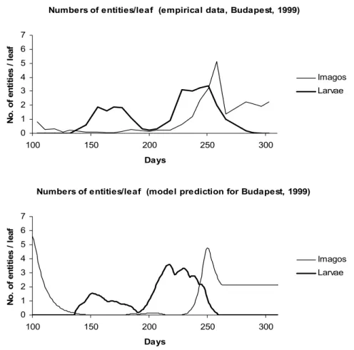
5. The number of entities does not change in the first case, while in the second one it is decreasing for phenophase Ph and increasing for phenophase Ph+1. The predictions of the model for the daily number of entities of each phenological phase can be seen in Figures 8 and 9. In order to compare the predictions with the empirical data we displayed the average numbers of entities referred to a leaf (Figure 10). It can be seen that the model follows the empirical data quite well. Its advantage is, however, that it gives such information about each single phenophase that has not been measured.
Numbers of entities/leaf (empirical data, Budapest, 1999)
0 1 2 3 4 5 6 7
100 150 200 250 300
Days
No. of entities / leaf
Imagos Larvae
Numbers of entities/leaf (model prediction for Budapest, 1999)
0 1 2 3 4 5 6 7
100 150 200 250 300
Days
No. of entities / leaf
Imagos Larvae
Figure 10. The numbers of Sycamore lace bug imagos and larvae per leaf in Budapest, between the 100th and the 300th days of year 1999
Upper figure: empirical data; Lower figure: model prediction
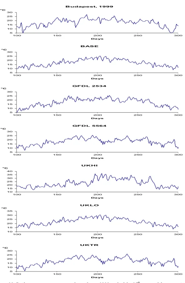
Budapest, 1999
5 10 15 20 25 30
100 150 200 250 300
Da ys
°C
BASE
5 10 15 20 25 30
100 150 200 250 300
Da ys
°C
GFDL 2534
5 10 15 20 25 30
100 150 200 250 300
Da ys
°C
GFDL 5564
5 10 15 20 25 30
100 150 200 250 300
Da ys
°C
UKHI
10 15 20 25 30 35 40
100 150 200 250 300
Da ys
°C
UKLO
10 15 20 25 30 35
100 150 200 250 300
Da ys
°C
UKTR
5 10 15 20 25 30
100 150 200 250 300
Da ys
°C
Figure 11. Daily average temperature data of year 1999 and of the 15th years of the scenarios.
Note that the scale of axis y of UKLO and UKHI is different because of the essentially higher values.
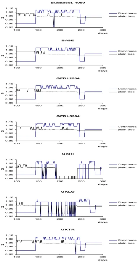
Budapest, 1999
0.85 0.90 0.95 1.00 1.05 1.10
100 150 200 250 300
da ys R
Corythuca plain tree
BASE
0,85 0,90 0,95 1,00 1,05 1,10
100 150 200 250 300
da ys R
Corythuca plain tree
GFDL2534
0,85 0,90 0,95 1,00 1,05 1,10
100 150 200 250 300
da ys R
Corythuca plain tree
GFDL5564
0,85 0,90 0,95 1,00 1,05 1,10
100 150 200 250 300
da ys R
Corythuca plain tree
UKHI
0,85 0,90 0,95 1,00 1,05 1,10
100 150 200 250 300
da ys R
Corythuca plain tree
UKLO
0,85 0,90 0,95 1,00 1,05 1,10
100 150 200 250 300
da ys R
Corythuca plain tree
UKT R
0,85 0,90 0,95 1,00 1,05 1,10
100 150 200 250 300
da ys R
Corythuca plain tree
Figure 12. Activity terms Rt of the 15th years of the scenarios. In order to see the effect of the climate better, we displayed the activity terms of Corythuca ciliata as well as the ones of
Sycamore trees.