Comparison of goodness measures for linear factor structures

(1)

Comparison of goodness measures for linear factor structures*

Borbála Szüle Associate Professor Insurance Education and Research Group, Corvinus University of Budapest E-mail: borbala.szule@uni- corvinus.hu

Linear factor structures often exist in empirical data, and they can be mapped by factor analysis. It is, however, not straightforward how to measure the goodness of a factor analysis solution since its results should correspond to various requirements. Instead of a unique indicator, several goodness measures can be defined that all contribute to the evaluation of the results.

This paper aims to find an answer to the question whether factor analysis outputs can meet several goodness criteria at the same time. Data aggregability (measured by the determinant of the correlation matrix and the proportion of explained variance) and the extent of latency (defined by the determinant of the anti- image correlation matrix, the maximum partial correlation coefficient and the Kaiser–Meyer–Olkin measure of sampling adequacy) are studied. According to the theoretical and simulation results, it is not possible to meet simultaneously these two criteria when the correlation matrices are relatively small. For larger correlation matrices, however, there are linear factor structures that combine good data aggregability with a high extent of latency.

KEYWORDS: Aggregation.

Indicators.

Model evaluation.

DOI: 10.20311/stat2017.K21.en147

* The author is grateful to the anonymous reviewer for the valuable comments.

(2)

L

inear factor structures are important in exploring empirical data. Factor analysis may reveal the underlying data patterns by providing information about such structures. If nonlinearity within data does not prevail, factor analysis may be appli- cable for several data analysis purposes. Theoretically, there is a distinction between confirmatory factor analysis (that is used to test an existing data model) and exploratory factor analysis (aimed at finding latent factors) (Sajtos–Mitev [2007]). Goodness measures (for example, the grade of reproducibility of correlations or the size of partial correlation coefficients) may be related to the specific purposes of factor analyses and contribute to the evaluation of results. This paper focuses on exploratory factor analysis, thus correlation values are of central importance in assessing model adequacy.

Exploratory factor analysis methods include common factor analysis and principal component analysis (Sajtos–Mitev [2007]), with the major difference that the latter is based on spectral decomposition of the (ordinary) correlation matrix, while the other applies different algorithms for calculating factors, for example, eigenvalues and eigenvectors of reduced correlation matrices are computed (as opposed to the unreduced ordinary correlation matrix). The application of a reduced correlation matrix in calculations (e.g. in principal axis factoring that is a factor analysis algorithm) emphasises the distinction between those common and unique factors that are assumed to determine measurable data. An exploratory factor solution is “good” when the spectral decomposition results in an uneven distribution of eigenvalues so that the (easily interpretable) eigenvectors are strongly correlated with the observable variables, with relatively low partial correlations between measurable variables. Consequently, some criteria (associated with the goodness of factor analysis results) can be formulated based on Pearson correlation coefficients and partial correlation values. In the paper, five correlation- related measures are defined, which are related to data aggregability and the extent of factor latency (as goodness criteria). Both of these criteria could be referred to as “a measure of sampling adequacy”, but to emphasise different aspects of goodness, the two sets of goodness measures of these criteria are analysed separately in the paper.

The correlation matrix determinant is one of such measures. It is a function of matrix values, and although it does not express all “information” inherent in the matrix, its lower values indicate good data aggregability, which refers to an adequate factor analysis solution. Since factor analysis solutions are usually associated with the eigenvalue-eigenvector decomposition of a matrix, the other measure of data aggregability in the paper is the proportion of explained variance (if the first factor is retained). For example, in principal component analysis, the correlation matrix can

(3)

be decomposed, and its eigenvalues correspond to the component variance values, thus the proportion of explained variance is the ratio of the variance (eigenvalue) of the retained component and total variance. In other factor analysis methods, similar calculations can be performed. Data aggregability is better, if the highest eigenvalue in the analysis (hence the calculated proportion of explained variance) is higher.

Factor analysis often aims to find latent variables that are not observable directly.

Therefore, besides data aggregability, the extent of latency is another important component in assessing factor analysis outputs. In the paper, three goodness measures (related to partial correlation) are used to assess this criterion.

Such as Pearson correlation coefficients, partial correlation values also describe a linear relationship between two observable variables (while controlling for the effects of other variables). The presence of latent factors in data may be indicated by a linear relationship of observable variables that are characterised by high Pearson correlation coefficients (in absolute terms) and low partial correlation values (also in absolute terms). Thus, the highest absolute value of partial correlations is considered as one of the goodness measures in the paper (lower values indicate better results than higher values).

In factor analysis, the total KMO (Kaiser–Meyer–Olkin) value and the anti-image correlation matrix summarise the most important information about partial correlations. For adequate factor analysis outputs, the total KMO value should be above a predefined minimum value (see, for example, Kovács [2011]), thus we use the total KMO value as another goodness measure in the paper (whose higher values indicate better results than lower values). The off-diagonal elements of the anti-image correlation matrix are the negatives of the partial correlation coefficients, while the diagonal values represent partial-correlation-related measures of sampling adequacy (variable-related KMO values) for observable variables (Kovács [2014]). If the determinant of the anti-image correlation matrix is high (for example, it is close to one), it may also be considered as an indicator of the goodness of a factor analysis solution.

Contributing to the literature, the paper is aimed at exploring whether these alter- native goodness criteria can be met simultaneously. Since the theoretical modelling of an arbitrary correlation matrix (without any assumption about the size of the matrix or the relationship of the values in the matrix) does not allow a parsimonious parametrisation of the model, some simplifications are introduced. For a selected small matrix size (three columns), both theoretical and simulation results are calculated and compared, and for larger correlation matrices the results of the numerical computations are demonstrated.

The paper is organised as follows. The first chapter introduces the simple theoretical assumptions of the paper, while the second summarises the theoretical and simulation results of the goodness measures. The last chapter presents conclusions and describes directions for future research.

(4)

1. The theoretical model

In exploratory factor analysis, factors can be considered as latent variables that, unlike observable variables, cannot be measured or observed (Rencher–Christensen [2012]). Interpretable latent variables may underlie not only cross sectional data but also time series (Fried–Didelez [2005]). The range of quantitative methods for the analysis of latent data structures is wide, for example, conditional dependence models for observed variables, in terms of latent variables, can also be presented with copulas (Krupskii–Joe [2013]).

The creation of latent variables can be performed by factor analysis with several algorithms, and a general feature of such an analysis is the central importance of (linear) Pearson correlation values during calculations. According to some authors (e.g. Hajdu [2003]), principal component analysis can be considered as a factor analysis method.

Despite important similarities, principal component analysis and other factor analysis methods exhibit certain differences: in principal component analysis the whole correlation matrix can be reproduced if all components are applied for the reproduction, while, for example, in principal axis factoring (which is another factor analysis method) theoretically only a reduced correlation matrix can be reproduced (in which the diagonal values are lower than one). This difference is connected to the dissimilarity of assumptions about the role of unique factors in determining measurable data. Principal axis factoring assumes that common and unique factors are uncorrelated, and the diagonal values of the reproduced correlation matrix are related solely to the common factors. In the case of principal component analysis, however, the effects of common and unique factors are modelled together (Kovács [2011]). The naming of eigenvectors also emphasises this difference: linear combinations of observable variables are called components in principal component analysis, while they are referred to as factors in principal axis factoring. In this paper, principal component analysis illustrates factor analysis, thus it is worth showing that the results of the principal component analysis and another factor analysis method (principal axis factoring) are similar. It can be demonstrated by a simple example (simulating 1 000 correlation matrices with three normally distributed variables) that the (Pearson) correlation between the factor and the component (both with the highest eigenvalue) is close to one (e.g. if all correlation values in the matrix are equal to 0.25, then it is approximately 0.9968 with 0.0035 standard deviation). Simula- tion is often performed to assess selected features of algorithms (Josse–Husson [2012]), Brechmann–Joe [2014]). Its results can be considered reliable because the problem that factor analysis results are sensitive to outliers (as described, for example, by Serneels–

Verdonck [2008] and Hubert–Rousseeuw–Verdonck [2009]), cannot be regarded serious in calculation, due to the distributional assumptions of this paper. Accordingly, principal component analysis (and the spectral decomposition of the ordinary correlation matrix) is used in the following to identify latent factors.

(5)

The size of the correlation matrix is an important parameter in analysis. An ordinary correlation matrix can be quite complex; there is only one theoretical restriction on its form: it should be a symmetric, positive semidefinite matrix. Since the complexity of a correlation matrix may increase with its size, first a simple example with three observable variables is examined. Even in this case, the requirement that the (ordinary) correlation matrix should be positive semidefinite allows several combinations of (Pearson) correlation values.

Assume, for example, that the correlation matrix (containing Pearson correlation values) is defined as follows:

1 2

1 3

2 3

1 1

1 r r

R r r

r r

 

 

  

 

 

. /1/

The former requirement is equivalent to presuming that the correlation matrix has only nonnegative eigenvalues. Assuming that the lowest eigenvalue of the correlation matrix in equation /1/ is indicated by λ₃, this eigenvalue can be calculated by using the formula:



1 λ3



³



1 λ3







r1² r2² r3²



  2 r r1 2 r3  0. /2/

Theoretically, the solution of equation /2/ could be a complex number (and then its interpretation in factor analysis could be problematic). However, given that all values in the correlation matrix are real numbers, the eigenvalues of the correlation matrix are also real numbers. As a solution of equation /2/, the lowest eigenvalue is described as follows:

2 2 2

1 2 3 1 2 3

3 2 2 2 3

1 2 3

1 2 cos 1 arccos

3 3

3

r r r r r r

λ

r r r

  

  

      

            . /3/

To illustrate that only certain combinations of correlation values are related to a positive semidefinite correlation matrix, assume that r₁ 0 in the following example. In this case, equation /3/ is equivalent to equation /4/:

2 2 2

1 2 3

3 1 2 cos .

3 6

r r r π

λ    

       /4/

(6)

By rearranging equation /4/, the condition for the positive semidefiniteness of the correlation matrix is described as:

r₂²  r₃²  1. /5/

Equation /5/ describes the possible combinations of correlation values for which the correlation matrix is positive semidefinite. Using different assumptions for the value of r₁, similar restrictions could be defined that describe a possible range for Pearson correlation values in the correlation matrix. Equations /4/ and /5/ can be interpreted as meaning that the relationships of Pearson correlation values in an (ordinary) correlation matrix should meet some requirements (as a consequence of the theoretical positive semidefiniteness of the correlation matrix).

For the sake of simplicity, it is assumed in our theoretical model that all off- diagonal elements in the ordinary correlation matrix are non-negative values that are equal (r r₁ r₂ r₃), and r 0. In this case, the lowest eigenvalue in equation /3/ is equal to 1 rsince under these simple assumptions the highest eigenvalue of the ordinary correlation matrix is equal to 1 2r, and the other two eigenvalues are equal to 1 r. Thus, the condition for the positive semidefiniteness of the correlation matrix is met. In the next chapter, the theoretical results associated with goodness measures are calculated under these simple assumptions. In the simulation analysis, these assumptions are relaxed.

2. Goodness measures in the model

The goodness of an exploratory factor analysis solution has several aspects, so the range of possible goodness measures is also relatively wide. For example, the Barlett’s test allows one to evaluate whether the sample correlation matrix differs significantly from the identity matrix (Knapp–Swoyer [1967], Hallin–Paindaveine–Verdebout [2010]) when all eigenvalues are equal (and thus the relevant eigenvectors cannot be interpreted as corresponding to latent factors). Theoretically, subsphericity (equality among some of the eigenvalues) could also be tested (Hallin–Paindaveine–Verdebout [2010]), and other eigenvalue-related goodness of fit measures (Chen–Robinson [1985]), for example, total variance explained by the extracted factors (Hallin–

Paindaveine–Verdebout [2010], Martínez-Torres et al. [2012], Schott [1996]) may also contribute to the assessment of factor models. Besides these aspects, interpretability of factors is another important question in goodness evaluation (Martínez-Torres et al.

[2012]) that should be considered when deciding about the number of extracted factors.

(7)

The selection of relevant factors (or components in a principal component analysis) may depend also on the objectives of the analysis (Ferré [1995]). If maximum likeli- hood parameter estimations can be performed, then, for example, Akaike’s information criterion or Bayesian information criterion may be applied when determining the factor number (Zhao–Shi [2014]). However, it should be emphasised that not all approaches to factor selection are linked to distributional assumptions (Dray [2008]); another possible method for factor extraction is to retain those factors (or components) whose eigenvalues are larger than one (Peres-Neto–Jackson–Somes [2005]). Despite the wide range of goodness measures, the comparison of factor analysis results is not simple, since factor loadings in different analyses cannot be meaningfully compared (Ehrenberg [1962]).

To compare selected goodness measures, results from a simple theoretical model and a simulation analysis are introduced. Note that although factor interpretability is an important component of “goodness”, this paper does not analyse the potential difficulties in the “naming” of factors.

Goodness of a factor structure can be evaluated based on ordinary and partial correlations. In the following, these figures are calculated in a theoretical model. Equa- tion /6/ shows a (symmetric and positive semidefinite) ordinary correlation matrix that corresponds to the simple theoretical assumptions of this paper.

1

1 1

 

 

  

 

 

r r

R r r

r r

/6/

The assumptions result in a nonnegative positive semidefinite matrix. Although an exact nonnegative decomposition of a nonnegative positive semidefinite matrix is not always available (Sonneveld et al. [2009]), all eigenvalues are nonnegative real numbers in our case. The following optimality measures are analysed and compared:

1. correlation matrix determinant; 2. proportion of the explained variance; 3. highest absolute value of the partial correlation; 4. total KMO value; 5. determinant of the anti-image correlation matrix.

The first two refer to data aggregability, while the last three indicate the extent of factor latency.

The correlation matrix determinant has been extensively studied in data analysis literature, for example, Olkin [2014] describes its bounds. Under the simple assumptions in this paper, the correlation matrix determinant is defined by equation /7/, as presented by the literature (e.g. Joe [2006]):

det

 

R  2 r³ 3 r² 1. /7/

(8)

Theoretically, the correlation matrix determinant is between zero and one, and the determinant of the unity matrix is equal to one. If the correlation matrix is a unity matrix, then all eigenvalues of the correlation matrix are one. In a factor analysis, this case would correspond to such a solution where the highest number of observable variables (that strongly correlate with a calculated factor) is only one. Thus, if the correlation matrix is a unity matrix, factor analysis solutions cannot be optimal. Based on these considerations, a lower (close to zero) correlation matrix determinant could indicate a better factor structure (that could be related to latent factors in data). In this paper, one of the goodness criteria of factor structures is the ordinary correlation matrix determinant:

the factor structure that belongs to the lowest correlation matrix determinant is the best.

Total variance is the sum of observed variables in a principal component analysis (if the analysis is based on the correlation matrix), and the proportion of the explained variance is the ratio of the sum of eigenvalues for retained components to total variance.

The latter can be considered as another measure of data aggregability. Since there are various rules for retaining factors, this goodness measure could be defined as the ratio of the highest eigenvalue (of the correlation matrix) to the number of observed variables.

In our simple theoretical model, this optimality measure is a linear function of the Pear- son correlation coefficient 1 2

3

   

 

 

r , thus its optimal value is r 1. Note, it is the same optimum that belongs to the criterion of the correlation matrix determinant.

Another aspect of the goodness of factor structures is associated with the partial correlation coefficients between observable variables. Partial correlations measure the strength of the relationship of two variables while controlling for the effects of other variables. In a good factor model, the partial correlation values are close to zero (Kovács [2011]).

Thus, in an optimal solution, the partial correlation coefficient with the highest absolute value would be theoretically zero.

The KMO measure of sampling adequacy is a partial-correlation-related measure that can be calculated for each variable separately or for all variables together. The KMO value is presented in equation /8/ (Kovács [2011]). If it is calculated for the variables separately (and if pairwise Pearson correlation values and partial correlation coefficients are indicated by r_ij and p_ij, respectively), then:

2

2 2

ij

i j

ij ij

i i i j

r

KMO r p



 

 



 

^. ^/8/

Theoretically, the maximum value of the KMO measure is one (if the partial correlation values are zero), and a higher KMO value indicates a better database for the

(9)

analysis (Kovács [2011]). Such as individual KMO values that are calculated for each variable separately, the total (database-level) KMO value (that takes all pairwise ordinary and partial correlation coefficients into account) can be calculated in a way similar to the one in equation /8/, if all pairwise partial and ordinal correlation coefficients are considered. For an adequate factor analysis solution, the total KMO value should be at least 0.5 (Kovács [2011]).

The anti-image correlation matrix summarises information about partial correlation coefficients: the diagonal values of the anti-image correlation matrix are the KMO measures of sampling adequacy (calculated for separate variables), and the off-diagonal elements are the negatives of the pairwise partial correlation coefficients. Equation /9/ shows the anti-image correlation matrix that corresponds to the model assumptions:

   

 

   

   

 

KMO p p

P p KMO p

p p KMO

. /9/

Under the assumptions in this paper, the variable-related KMO values are equal for each variable and described as follows:

 

2 2

1

1 1

 

 

KMO r

r

. /10/

Equation /10/ shows that the variable-related and the total KMO values are higher than 0.5 in the simple theoretical model. Thus, our factor analysis solution is adequate.

The pairwise partial correlation coefficients are also equal in the simple model framework, and can be expressed as a function of the Pearson correlation values, as it is described by equation /11/:

 1

 p r

r . /11/

As the former equation shows, the partial correlation value in the theoretical model may not be equal to zero unless the off-diagonal values of the correlation matrix are zero. This result means that in the case of the assumed, relatively small correlation matrix, the optimum value for r (the Pearson correlation value in the correlation matrix) that is relevant to partial correlations cannot be equal to the optimum value for r associated with the correlation matrix determinant.

(10)

Although the partial correlation value is an increasing function of the Pearson correlation value in the correlation matrix of the theoretical model, it is also worth analysing the anti-image matrix that summarises information about all ordinary and partial correlation values. As indicated by equation /12/, the determinant of the anti- image correlation matrix can be expressed as a function of the Pearson correlation values (indicated by r in the model), based on equations /10/ and /11/:

   

 

   

2 3 3 2 2

2 3 2 2

1 1

det 2 3

1 1 1 1 1 1

   

 

            

r r r r

P

r r r r . /12/

As far as partial correlation values are concerned, theoretically, the pairwise partial correlation coefficients are zero when the factor structure is optimal, which results in KMO values that all equal one. In this case, the anti-image correlation matrix was a unity matrix with a determinant that is equal to one. Based on these considerations, the determinant of the anti-image correlation matrix can be regarded as another goodness criterion: the best factor structure is linked to the highest determinant value.

After the comparison of the goodness measures in the theoretical model, the research can be extended with a simulation analysis to cover all possible combinations of the matrix elements (for the given matrix size) that result in a positive semidefinite correlation matrix. As Lewandowski–Kurowicka–Joe [2009] point out, the speed of calculations is an important aspect in generating a set of random correlation matrices.

In this paper, the elements of (symmetric) matrices are generated as uniformly distributed random variables that are between –1 and 1, and the positive semidefinite matrices are considered as simulated correlation matrices. In this simulation method, the probability that the simulation results in a positive semidefinite correlation matrix decreases with the matrix size. For example, Böhm–Hornik [2014] show that the probability of positive definiteness of a symmetric n n matrix with unit diagonal and upper diagonal elements distributed identically and independently with a uni- form distribution (on –1,1) is approximately 0.61685 for n 3 (and the probability is close to zero for n 10). In our study, the simulation method resulted in 6 171 random correlation matrices for n 3 (with 10 000 total matrix simulations), which are analysed in the following.

To compare the two data aggregability measures, Figure 1 illustrates their relationship (if the first factor is retained) for those (2 294) cases in the simulation analysis when the total KMO value is higher than 0.5. Both theoretical and simulation results show that these measures are similar, and there are factor structures that meet the aggregability criterion (when the correlation matrix determinant is close to zero and the proportion of explained variance is close to one).

(11)

Figure 1. Comparison of the correlation matrix determinant and the proportion of explained variance

0.0 0.1 0.2 0.3 0.4 0.5 0.6 0.7 0.8 0.9 1.0

0.0 0.2 0.4 0.6 0.8 1.0

Correlation matrix determinant

Variance explained

Simulated data Theoretical model Source: Here and hereafter, own calculations.

In the following, the relationship between the correlation matrix determinant rep- resenting the extent of data aggregability and other (factor-latency-related) goodness measures is studied (taking the KMO-related constraint into account).

Since KMO can be considered as a relatively simple measure of factor latency, it is worth studying other factor latency measures to decide whether a factor solution meets the two optimality criteria. Figure 2 illustrates the relationship of the absolute value of the maximum partial correlation coefficient and the correlation matrix determinant.

Figure 2. Comparison of the correlation matrix determinant and the absolute value of the maximum partial correlation coefficient

0.0 0.1 0.2 0.3 0.4 0.5 0.6 0.7 0.8 0.9 1.0

0.0 0.2 0.4 0.6 0.8 1.0

Maximum partial correlation

Correlation matrix determinant Simulated data Theoretical model

(12)

Figure 2 suggests that for linear factor structures it may be difficult to meet both data aggregability and factor-latency-related requirements simultaneously. As equation /11/ shows, the maximum partial correlation coefficient grows in the theoretical model if the Pearson correlation coefficient increases, while the simulation results revealed a similar relationship between the maximum partial correlation coefficient and the correlation matrix determinant.

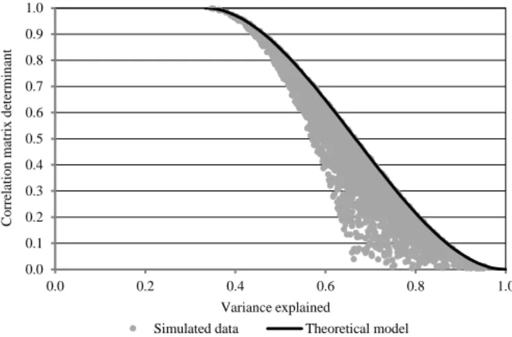
Since the anti-image correlation matrix summarises information about partial correlation coefficients, the determinant of this matrix may also be considered as a measure of the extent of factor latency. Figure 3 illustrates the relationship and differences between the determinant of the correlation matrix and that of the anti-image correlation matrix.

Figure 3. Comparison of two matrix determinants

–0.8 –0.7 –0.6 –0.5 –0.4 –0.3 –0.2 –0.1 0.0 0.1 0.2 0.3

0.0 0.2 0.4 0.6 0.8 1.0

Determinant of the anti-image correlation matrix

Correlation matrix determinant Simulated data Theoretical model

Note. The simulation results include those cases where the total KMO value is above 0.5.

According to the theoretical results, the correlation matrix determinant reaches its minimum value when the Pearson correlation between variables is equal to one, while the determinant of the anti-image correlation matrix reaches its maximum at a Pearson correlation value lower than one. Figure 3 also shows there is no factor solution that is “good enough” regarding both data aggregability and the extent of factor latency, if the KMO-related constraint is also taken into account: the anti-image correlation matrix determinant is not close to one if the correlation matrix determinant is close to zero.

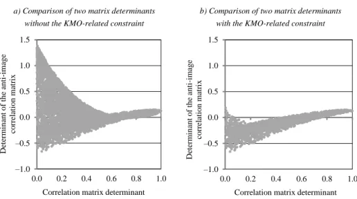
Figure 4 illustrates the effect of the KMO-related constraint: if it is not taken into account (and the number of the random correlation matrices is 6 171 in the simulation analysis), then it is possible to find linear factor structures for which the anti- image correlation matrix determinant is close to one while the correlation matrix

(13)

determinant is close to zero. However, if the KMO-related constraint is considered (and the number of the random correlation matrices is 2 294 in the simulation analysis), then no linear factor structures meet both goodness criteria.

Figure 4. Effect of the KMO-related constraint a) Comparison of two matrix determinants

without the KMO-related constraint

–1.0 –0.5 0.0 0.5 1.0 1.5

0.0 0.2 0.4 0.6 0.8 1.0

b) Comparison of two matrix determinants with the KMO-related constraint

–1.0 –0.5 0.0 0.5 1.0 1.5

0.0 0.2 0.4 0.6 0.8 1.0

Since the KMO measure of sampling adequacy can be considered as an important measure of the extent of factor latency, one can conclude that there are no factor structures that meet both criteria (data aggregability and the extent of factor latency) in the case of a relatively small correlation matrix (having three columns). The results for partial correlation with maximum absolute value also support this conclu- sion.

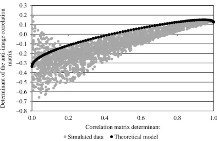
To explore the effects of relaxing the assumption about matrix size, correlation matrices with a simple structure are analysed: such as in equation /6/, it is presumed that all Pearson correlation values in a correlation matrix are equal. In this case, all off-diagonal values in the anti-image correlation matrix and the individual KMO values (the diagonal values of the anti-image correlation matrix) are also equal. Figure 5 illustrates the relationship between the (ordinary) correlation matrix determinant and the anti-image correlation matrix determinant for different Pearson correlation values (in the ordinary correlation matrix) and for different matrix sizes.

In Figure 5, the (Pearson) correlation values increase from 0.01 to 0.99 for each matrix size. If the correlation matrix size (indicated by n) is bigger, then the relationship of the two matrix determinants changes, but in none of the examined cases is the determinant of the anti-image correlation matrix close to one.

(14)

Figure 5. Effect of the correlation matrix size

–0.4 –0.3 –0.2 –0.1 0.0 0.1 0.2

0.0 0.2 0.4 0.6 0.8 1.0

n = 3 n = 5 n = 25

Note. In the figure, n indicates the size of the correlation matrix.

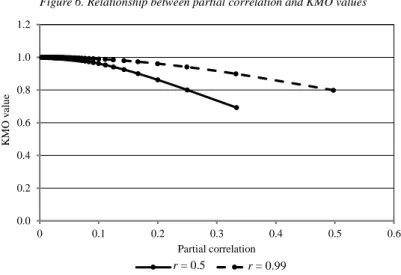
Figure 6. Relationship between partial correlation and KMO values

0.0 0.2 0.4 0.6 0.8 1.0 1.2

0 0.1 0.2 0.3 0.4 0.5 0.6

KMO value

Partial correlation r = 0.5 r = 0.99 Note. In the figure, r indicates the Pearson correlation value.

Figure 6 presents the relationship between partial correlation and KMO values if the matrix size increases from 3 to 250 columns (variables), for two different Pearson correlation values. It indicates that if the correlation matrix is relatively large, then the partial correlation values are close to zero, while the KMO values are around one. For example, if the Pearson correlation values in the (ordinary) correlation matrix are all equal to 0.99, then in a large correlation matrix (e.g. with 250 variables) the partial correlation values

n = 3 n = 5 n = 25

r = 0.5 r = 0.99

(15)

are nearly zero, and the KMO values are close to one. This example shows a correlation matrix solution that is appropriate for meeting both criteria. The result also suggests that if the extent of latency should be expressed with one value, then this could be the determinant of a modified version of the anti-image correlation matrix (instead of the determinant of the frequently analysed anti-image correlation matrix).

3. Conclusions

In parallel with the development of information technologies, the amount of em- pirically analysable data has grown over the last decades, and the need for advanced pattern recognition techniques has increased, too. In data, linear factor structures may be present, and latent factors can be identified by various factor analysis methods.

The evaluation of the goodness of such factor structures is thus a compelling issue of research. This paper aims to contribute to the literature by examining whether linear factor structures can meet multiple requirements simultaneously.

Factor analysis methods are connected to the measurement of the strength of linear relationships between observable variables. The ordinary correlation matrix that contains information about such relationships can be quite complex since there are only two theoretical restrictions on its form: it should be symmetric and positive semidefinite. Partly because of the complexity of correlation matrices, various goodness measures can be defined for the evaluation of factor analysis results. This paper has examined two criteria: data aggregability (measured by the determinant of the (ordinary) correlation matrix and the proportion of explained variance) and the extent of factor latency (defined by the total KMO value, the maximum partial correlation coefficient and the determinant of the anti-image correlation matrix).

Note that in the paper goodness was analysed only from a mathematical point of view (whether goodness criteria can be met simultaneously); in practical applications, however, other aspects (for example, the possibility of “naming” the factors) may also be considered when evaluating a factor structure.

The paper contributes to the literature with the concurrent examination of two goodness criteria. First, a relatively small correlation matrix (having three columns) was analysed with theoretical modelling and simulation analysis. The results of both methods show that the defined criteria cannot be met simultaneously. This outcome can be associated with the relationship between the Pearson correlation values (between observable variables) and the pairwise partial correlation coefficients: according to the theoretical model, increase in the pairwise Pearson correlation values is accompanied by the growth of the partial correlation coefficients. The paper also

(16)

suggests that if the correlation matrix is large, the increase in the extent of partial correlations is less significant, and one can identify factor structures that meet both data aggregability and latency criteria (measured with the value of partial correlations). The results may also be interpreted in such a way that if the extent of latency should be expressed with one value, then it could be the determinant of a modified version of the anti-image correlation matrix (instead of the determinant of the frequently analysed anti-image correlation matrix).

The goodness of linear factor structures has several aspects whose further analysis can be subject of future research. The model presented in this paper may be extended, for example, by modifying the definition of the goodness criteria, or by formulating a more general set of assumptions for the elements in the ordinary correlation matrix.

References

BÖHM,W.–HORNIK,K. [2014]: Generating random correlation matrices by the simple rejection method: why it does not work. Statistics and Probability Letters. Vol. 87. April. pp. 27–30.

https://doi.org/10.1016/j.spl.2013.12.012

BOIK,R.J. [2013]: Model-based principal components of correlation matrices. Journal of Multivar- iate Analysis. Vol. 116. April. pp. 310–331. https://doi.org/10.1016/j.jmva.2012.11.017 BRECHMANN,E.C.–JOE, H. [2014]: Parsimonious parameterization of correlation matrices using

truncated vines and factor analysis. Computational Statistics and Data Analysis. Vol. 77. Sep- tember. pp. 233–251. https://doi.org/10.1016/j.csda.2014.03.002

CHEN,K.H.–ROBINSON, J. [1985]: The asymptotic distribution of a goodness of fit statistic for factorial invariance. Journal of Multivariate Analysis. Vol. 17. Issue 1. pp. 76–83.

https://doi.org/10.1016/0047-259X(85)90095-8

DRAY,S. [2008]: On the number of principal components: a test of dimensionality based on meas- urements of similarity between matrices. Computational Statistics & Data Analysis. Vol. 52.

Issue 4. pp. 2228–2237. https://doi.org/10.1016/j.csda.2007.07.015

EHRENBERG,A.S.C. [1962]: Some questions about factor analysis. Journal of the Royal Statistical Society. Series D (The Statistician). Vol. 12. No. 3. pp. 191–208.

https://doi.org/10.2307/2986914

FERRÉ,L. [1995]: Selection of components in principal component analysis: a comparison of methods. Computational Statistics & Data Analysis. Vol. 19. Issue 6. pp. 669–682.

https://doi.org/10.1016/0167-9473(94)00020-J

FRIED,R.–DIDELEZ,V. [2005]: Latent variable analysis and partial correlation graphs for multivariate time series. Statistics & Probability Letters. Vol. 73. Issue 3. pp. 287–296.

https://doi.org/10.1016/j.spl.2005.04.002

HAJDU,O. [2003]: Többváltozós statisztikai számítások. Központi Statisztikai Hivatal. Budapest.

HALLIN,M.–PAINDAVEINE,D.–VERDEBOUT, T. [2010]: Optimal rank-based testing for principal components. The Annals of Statistics. Vol. 38. No. 6. pp. 3245–3299.

https://doi.org/10.1214/10-AOS810

(17)

HUBERT,M.–ROUSSEEUW,P.–VERDONCK,T. [2009]: Robust PCA for skewed data and its outlier map. Computational Statistics and Data Analysis. Vol. 53. Issue 6. pp. 2264–2274.

https://doi.org/10.1016/j.csda.2008.05.027

JOE, H. [2006]: Generating random correlation matrices based on partial correlations. Journal of Multivariate Analysis. Vol. 97. Issue 10. pp. 2177–2189. https://doi.org/10.1016/

j.jmva.2005.05.010

JOSSE,J.–HUSSON, F. [2012]: Selecting the number of components in principal component analysis using cross-validation approximations. Computational Statistics and Data Analysis. Vol. 56.

Issue 6. pp. 1869–1879. https://doi.org/10.1016/j.csda.2011.11.012

KNAPP,T.R.–SWOYER,V. H. [1967]: Some empirical results concerning the power of Bartlett’s test of the significance of a correlation matrix. American Educational Research Journal. Vol. 4.

Issue 1. pp. 13–17.

KOVÁCS,E. [2011]: Pénzügyi adatok statisztikai elemzése. Tanszék Kft. Budapest.

KOVÁCS,E. [2014]: Többváltozós adatelemzés. Typotex. Budapest.

KRUPSKII,P.–JOE,H. [2013]: Factor copula models for multivariate data. Journal of Multivariate Analysis. Vol. 120. September. pp. 85–101. https://doi.org/10.1016/j.jmva.2013.05.001 LEWANDOWSKI,D.–KUROWICKA,D.–JOE, H. [2009]: Generating random correlation matrices

based on vines and extended onion method. Journal of Multivariate Analysis. Vol. 100. Issue 9.

pp. 1989–2001. https://doi.org/10.1016/j.jmva.2009.04.008

MARTÍNEZ-TORRES,M.R.–TORAL,S.L.–PALACIOS,B.–BARRERO, F. [2012]: An evolutionary factor analysis computation for mining website structures. Expert Systems with Applications.

Vol. 39. October. pp. 11623–11633. http://dx.doi.org/10.1016/j.eswa.2012.04.011

OLKIN,I. [2014]: A determinantal inequality for correlation matrices. Statistics and Probability Letters. Vol. 88. pp. 88–90. https://doi.org/10.1016/j.spl.2014.01.012

PERES-NETO,P.R.–JACKSON,D.A.–SOMERS,K. M. [2005]: How many principal components?

Stopping rules for determining the number of non-trivial axes revisited. Computational Statis- tics & Data Analysis. Vol. 49. Issue 4. pp. 974–997. http://dx.doi.org/10.1016/

j.csda.2004.06.015

RENCHER,A.C.–CHRISTENSEN, W. F. [2012]: Methods of Multivariate Analysis. Third Edition.

Wiley & Sons Inc. Hoboken.

SAJTOS,L.–MITEV,A. [2007]: SPSS kutatási és adatelemzési kézikönyv. Alinea Kiadó. Budapest.

SCHOTT, J.R. [1996]: Eigenprojections and the equality of latent roots of a correlation matrix.

Computational Statistics & Data Analysis. Vol. 23. Issue 2. pp. 229–238.

https://doi.org/10.1016/S0167-9473(96)00033-3

SERNEELS,S.–VERDONCK, T. [2008]: Principal component analysis for data containing outliers and missing elements. Computational Statistics & Data Analysis. Vol. 52. Issue 3. pp. 1712–1727.

SONNEVELD,P.– VAN KAN,J.J.I.M.–HUANG,X.–OOSTERLEE, C. W. [2009]: Nonnegative matrix factorization of a correlation matrix. Linear Algebra and its Applications. Vol. 431. Issues 3–4.

pp. 334–349. https://doi.org/10.1016/j.laa.2009.01.004

ZHAO,J.–SHI, L. [2014]: Automated learning of factor analysis with complete and incomplete data. Computational Statistics and Data Analysis. Vol. 72. April. pp. 205–218.