Data acquisition and integration 1.

(1)

Data acquisition and integration 1.

The basics of positioning

Ferenc Végső

(2)

Data acquisition and integration 1.: The basics of positioning

Ferenc Végső Lector: Árpád Barsi

This module was created within TÁMOP - 4.1.2-08/1/A-2009-0027 "Tananyagfejlesztéssel a GEO-ért"

("Educational material development for GEO") project. The project was funded by the European Union and the Hungarian Government to the amount of HUF 44,706,488.

v 1.0

Publication date 2010

Summary: in this chapter discussed on the shape of the Earth, the approximations of the Earth’s surface, the problem of the vertical datum, earth coordinate systems, projected coordinate system, map projections, distortions of projections and geographic transformations.

The right to this intellectual property is protected by the 1999/LXXVI copyright law. Any unauthorized use of this material is prohibited. No part of this product may be reproduced or transmitted in any form or by any means, electronic or mechanical, including photocopying, recording, or by any information storage and retrieval system without express written permission from the author/publisher.

(3)

Chapter 1. The basics of positioning

1. 1.1 Introduction

The goal of positioning is to mapping points or objects determined on the natural surface of the Earth on a flat paper (or 2D Cartesian coordinate system) with minimal distortions.

Figure 1. The schematic flow diagram of positioning

In this chapter, we are dealing with history of the Earth shape and the Earth shape representations. The expression figure of the Earth has various meanings according to the way it is used and the precision with which the Earth's size and shape is to be defined. The actual topographic surface is most apparent with its variety of land forms and water areas. This is, in fact, the surface on which actual Earth measurements are made. It is not suitable, however, for exact mathematical computations, because the formulas which would be required to take the irregularities into account would necessitate a prohibitive amount of computations. The topographic surface is generally the concern of topographers and hydrographers. The Pythagorean concept of a spherical earth offers a simple surface, which is mathematically easy to deal with. Many astronomical and navigational computations use it as a surface representing the Earth. While the sphere is a close approximation of the true figure of the Earth and satisfactory for many purposes, to the geodesists interested in the measurement of long distances—

spanning continents and oceans—a more exact figure is necessary. Local approximations of the Earth’s shape means local reference ellipsoids. The idea of a planar or flat surface for Earth, however, is still acceptable for surveys of small areas. Plane surveys are made for relatively small areas, and no account is taken of the curvature of the Earth. A survey of a city would likely be computed as though the Earth were a plane surface the size of the city. For such small areas, exact positions can be determined relative to each other without considering the size and shape of the Earth.

(6)

Figure 2. Earth as seen in Valencia, Spain (Playa de la Malvarrosa)

1

In the 20th century, research across the geosciences contributed to drastic improvements in the accuracy of the Figure of the Earth. The ESA (European Space Agency) launched on 2009 March the Gravity field and Ocean Circulation Explorer (GOCE) satellite. The model of Fig. 3 is made by satellite measured gravity changes. An accurate model of the Earth's gravity field is crucial for defining exactly what height above sea level actually means. With this method, scientists will be able to say if two points are at the same height everywhere on the surface of the Earth.

Figure 3. The true shape of the Earth

1.1. 1.1.1 Approximation of Earth’s shape

The geoid is that equipotential surface which would coincide exactly with the mean ocean surface of the Earth, if the oceans were in equilibrium, at rest, and extended through the continents. It is the "mathematical figure of the Earth" (described by Gauss), a smooth but highly irregular surface that corresponds not to the actual surface of the Earth's crust. This surface can only be known through extensive gravitational measurements. Despite being an important concept for almost two hundred years in the history of geodesy and geophysics it has only been defined to high precision in recent decades. It is often described as the true physical figure of the Earth, in contrast to the idealized geometrical figure of a reference ellipsoid.

The next figure shows the context of geoid and the topographic surface:

1 http://en.wikipedia.org/wiki/File:Depositos_curvatura_mar300p.jpg

(7)

2

1. Ocean

2. Reference ellipsoid 3. Local plumb line 4. Continent 5. Geoid

The figure bottom interprets the differences – called undulation – between geoid and WGS84 ellipsoid on a world map.

Figure 4. Undulations on the surface of the Earth

3

2 http://en.wikipedia.org/wiki/File:Geoida.svg

3 http://en.wikipedia.org/wiki/File:Geoid_height_red_blue.png

(8)

The biggest known undulations are the minimum in the Indian Ocean with -100 meters and the maximum in the northern part of the Atlantic Ocean with +70 meters (figure above).

As mentioned above, the geoid is very complex surface, derived from gravity measurements. For surveying and positioning the more useful surface is an ellipsoid, which is mathematically correct form. Since the Earth is flattened at the poles and bulging at the equator, the geometrical figure used in geodesy to most nearly approximate Earth's shape is a spheroid or flattened ellipsoid of revolution. The ellipsoid of revolution is created by rotating an ellipse about its minor axis. A spheroid describing the figure of the Earth is called a reference ellipsoid. The reference ellipsoid for the Earth is called Earth ellipsoid.

Two numbers uniquely define an ellipsoid of revolution. Geodesists, by convention, use the semi major axis and flattening. The size is represented by the radius at the equator—the semi major axis of the cross-sectional ellipse—and designated by the letter a. The shape of the ellipsoid is given by the flattening, f, which indicates how much the ellipsoid departs from sphere. (In practice, the two defining numbers are usually the equatorial radius and the reciprocal of the flattening, rather than the flattening itself; for the WGS84 spheroid used by today's GPS systems, the reciprocal of the flattening is set at 298.257223563 exactly.)

The difference between a sphere and a reference ellipsoid for Earth is small, only about one part in 300.

Historically flattening was computed from grade measurements. Nowadays geodetic networks and satellite geodesy are used. In practice, many reference ellipsoids have been developed over the centuries from different surveys. The flattening value varies slightly from one reference ellipsoid to another, reflecting local conditions and whether the reference ellipsoid is intended to model the entire earth or only some portion of it. The axis of ellipsoid is approximately aligned with the rotation axis of the Earth. The ellipsoid is defined by the equatorial axis a and the polar axis b; their difference is about 21 km or 0,3 per cent. Additional parameters are the mass function J2, the correspondent gravity formula, and the rotation period (usually 86164 seconds).

During the time, the different sets of data used in national surveys are several of special importance: the Bessel ellipsoid of 1841, the international Hayford ellipsoid of 1924, Krassowski 1940, IUGG 67 and (for GPS positioning) the WGS84 ellipsoid.

The following table lists nine ellipsoids, which were the best estimation of the Earth's figure:⁴

Name Equatorial axis (m)

Polar axis (m) Inverse flattening

Delambre, France 1810

6,376985.0 308,6465

Airy 1830 6,377,563.4 6 356,256.91 299.3249646

Bessel 1841 6,377,397.155 6,356,078.963 299.1528128

Alexander Ross Clarke

6,378,206.4 6,356,583.8 294.9786982

Helmert 1906 6,378,200.0 (close to WGS84!) 298.30

International 1924

6,378,388.0 6,356,911.9 297.0

Krassowski 1940

6,378,245.00 (for Eastern Europe)

298.3

IUGG 1967, Luzern

6,378,165.00 (incl.

Sat.Geodesy)

298.25

4 http://en.wikipedia.org/wiki/Earth_ellipsoid

(9)

WGS 1984 6,378,137.00 6,356,752.3142 298.257223563

Earth ellipsoid and reference (local) ellipsoids

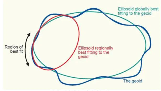
A data set, which describes the global average of the Earth’s surface curvature, is called the mean Earth Ellipsoid. The meridional curvature of the geoid close to the mean sea level, and therefore an ideal Earth ellipsoid has the same volume as the geoid. While the mean Earth ellipsoid is the ideal basis of global geodesy like measuring crustal movements, a so called reference or local ellipsoid may be the better choice. When geodetic measurements have to be computed on a mathematical reference surface, this surface should have a similar curvature as the regional geoid. Otherwise, the reduction of the measurements would get small distortions.

Figure 5. Global vs. local ellipsoid

5

The reason for using local ellipsoids: the coordinates of millions of boundary stones should remain fixed for a long period. If their reference surface would change, the coordinates themselves would also change. However, for international networks, GPS positioning or astronautics, these regional reasons are less relevant. As the knowledge of Earth's figure is increasingly accurate by the satellite gravity measuring, the International Union of Geodesy and Geophysics usually adopts the axes of the Earth ellipsoid to the best available data.⁶

The sphere

A sphere is a perfectly round geometrical object in three-dimensional space, such as the shape of a round ball.

Like a circle in two dimensions, a perfect sphere is completely symmetrical around its center, with all points on the surface lying the same distance r from the center point. This distance r is known as the radius of the sphere.

The maximum straight distance through the sphere is known as the diameter of the sphere. It passes through the center and is thus twice the radius.

5 http://www.kartografie.nl/geometrics/Reference%20surfaces/refsurf.html

6 http://en.wikipedia.org/wiki/Earth_ellipsoid

(10)

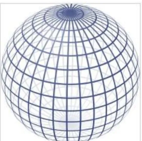
Figure 6. A two dimensional perspective picture of sphere

The Gaussian sphere provides a third-order approximation of the gravity field in the vicinity of the origin. The differences between an ellipsoid, which is a second-order approximation of the gravity field, and a Gaussian sphere as reference surfaces are negligible for national or regional mapping projects.

Figure 7. Locally suited Gauss sphere

7

Instead of using the ellipsoid, the sphere might be sufficient for much mapping tasks. In practice, maps at scale 1:5,000,000 or smaller can use the mathematically simpler sphere without the risk of large distortions.

2. 1.2 The problem of vertical datum

A vertical datum is used for measuring the elevations of points on the Earth's surface. Vertical datums are either tidal, based on sea levels, or geodetic, based on the same ellipsoid models of the earth used for computing horizontal datums. In common usage, elevations are often cited in height above sea level, although what ―sea level‖ actually means is a more complex issue than might at first be thought: the height of the sea surface at any one place and time is a result of numerous effects, like: waves, wind and currents, atmospheric pressure, tides, topography, and even differences in the strength of gravity due to the presence of mountains and enormous masses under the sea level.

For the purpose of measuring the height of objects on land, the usual datum used is Mean Sea Level. This is determined by measuring the height of the sea surface over a long period (preferably around 18 years, to account for all the astronomical effects that contribute to tide levels). This allows an average sea level to be determined, with the effects of waves, tides, and short-term changes in wind and currents removed. It will not remove the effects of local gravity strength, and so the height of MSL, relative to a geodetic datum, will vary around the world, and even around one country. For this reason, a country will choose the mean sea level at one specific point to be used as the standard ―sea level‖ for all mapping and surveying in that country. (For example, in

7 http://www.aps.anl.gov/Science/Publications

(11)

Hungary, the national vertical datum, named ―Balti‖, is based on what was mean sea level on tidal-pole meter at Kronstadt).

Figure 8. Tidal - pole meter at Kronstadt

Previously (before1960) was used in Hungary another vertical datum, named ―Adria‖, so there is can be find two type of vertical datum on old Hungarian maps.

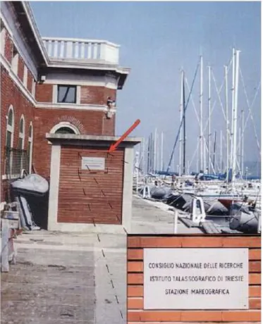
Figure 9. Building of Triest tidal – pole meter at Molo Sartorio (Italy)

(12)

Obviously, there are several realizations of local mean sea levels in the world. They are parallel to the Geoid but offset by up to a couple of meters. The local vertical datum is implemented through a leveling network.

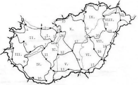
Figure 10. The first order Hungarian levelling network

8

A leveling network consists of benchmarks, whose height above mean sea level has been determined through geodetic leveling. The implementation of the datum enables easy user access. The surveyors do not need to start from scratch (i.e. from the Kronstadt tide-gauge) every time they need to determine the height of a new point.

They can use the benchmark of the leveling network that is closest to the point of interest.

Figure 11. The principle of leveling

9

The development of satellite based Global Positioning System (GPS) has facilitated the more accurate, more practical and economic use in geodesy and surveying professions. Today GPS serves the very wide range of geodetic applications ranging from monitoring earth crustal deformation to building the basis for GIS (Geographical Information System). It is necessary to transform the ellipsoidal heights to orthometric heights and this procedure is managed with the fundamental mathematical relationship between the two height systems.

8 http://www.fomi.hu/honlap/magyar/szaklap/1999/02/1991_02_4.htm

9 http://www.fao.org/docrep/field/003/e7171e/E7171E03.htm

(13)

Figure 12. Relationship between orthometric, ellipsoidal height and geoid undulation

10

Because of satellite gravity missions, it is currently possible to determine the orthometric height with centimeter level accuracy. It is foreseeable that a global vertical datum may become ubiquitous in the next 10-15 years. If all published maps are also using this global vertical datum by that time, heights will become globally comparable, effectively making local vertical datums redundant for GIS users.¹¹

3. 1.3 Earth coordinate systems

To positioning objects on the surface of the earth, we need a reference system. In geodesy, we make it in a geocentric coordinate system. Geocentric coordinates are an Earth-centered system of locating objects in three-dimensions along the Cartesian X, Y and Z-axes.

Figure 13. Geocentric coordinate system

12

We have drawn a circle around the Earth that intersects both the x-axis and y-axis and named that the equator.

We have also drawn a line from the North Pole to the South Pole that intersects the x-axis and named that the Greenwich Meridian. By the origin of our coordinate system is at the center of the Earth, it is a geocentric coordinate system.

10 http://www.kartografie.nl/geometrics/Reference%20surfaces/refsurf.html

11 R. Knippers: Geometric aspects of mapping

12 http://cfis.savagexi.com/2006/04/23/geocentric-coordinate-systems

(14)

They are differentiated from topocentric coordinates, which use the observer's location as the reference point for bearings in altitude and azimuth. Both systems share a common difficulty in that the Earth is constantly moving, which requires the addition of a time component to fix features on the surface of the Earth.

Figure 14. Topocentric coordinate system

13

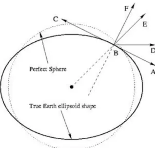
When we start marking down values until at some point we realize things are not looking well. In fact, at 45 degrees north (approximately how far north for example Hungary) our locations are off by around 18 kilometers. But why? Remember, because the Earth is not a perfect sphere. The north pole and south pole are slightly squished in. They are each about 18 kilometers closer to the center of the earth than you would expect with a perfect sphere.

The next picture shows the problem geometrically:

Figure 15. Geocentric vs. Geodetic coordinates

14

In geocentric coordinate system, we would calculate latitude as the angle lines DBE. However, if we are on the Earth's surface, it is useful to calculate latitude as the angle DBF where F is pointing straight up. In fact, the angle DBF is what we commonly called latitude. However, since the Earth is slightly flat, the line FB does not intersect the Earth's surface.

13http://cfis.savagexi.com/2006/04/23/geocentric-coordinate-systems

14 http://www.flightgear.org/Docs/Scenery/CoordinateSystem/CoordinateSystem.html

(15)

4. 1.4 Projected coordinate systems

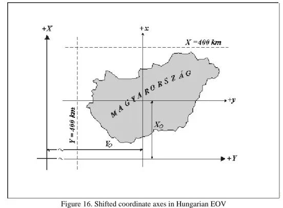
For a relative small pieces of Earth (like countries, regions, cities) the most useful mapping method is a projected coordinate system. The projected coordinate system has constant lengths, angles, and areas across the two dimensions. The x coordinate is usually the eastward direction of a point (northward in Hungary), and the y coordinate is usually the northward direction of a point (eastward in Hungary). The intersection of the x and y- axes is the origin and usually has a coordinate of (0, 0), or shifted like in Hungary to avoid mistakes in coordinates.

Figure 16. Shifted coordinate axes in Hungarian EOV

15

The projected coordinate system on maps represented for example as km lines.

15 http://www.agt.bme.hu/varga/Osszes/Dok3uj.htm

(16)

Figure 17. Grid lines on a topographic map

16

5. 1.5 Map projections

A map projection is any method of representing the surface of the Earth on a plane. Map projections are necessary for creating maps. All map projections distort the surface in some fashion. Depending on the purpose of the map, some distortions are acceptable and others are not; therefore, different map projections exist in order to preserve some properties of the sphere-like body at the expense of other properties (angle, distance, area).

There is no limit to the number of possible map projections.¹⁷

5.1. 1.5.1 Main types of projection

Conic projection

The conic, equal area map projection uses two or more standard parallels reduced (secant conic projection).

Although scale and shape are not preserved, distortion is minimal between the standard parallels.

18

16 http://lazarus.elte.hu/hun/dolgozo/zentail/ut/apatity/other/p1010134.jpg

17 http://en.wikipedia.org/wiki/Map_projection

18 http://webhelp.esri.com/arcgisdesktop/9.2/index.cfm?TopicName=Projection_types%3A_illustrated

(17)

Figure 18. Conic and secant conic projection

19

Example of secant conic projection:

20

Conic—mathematically projected on a cone conceptually secant at two standard parallels. One of the most widely used map projections in the United States today. Retains conformality. Distances true only along standard parallels; reasonably accurate elsewhere in limited regions. Directions reasonably accurate. Distortion of shapes and areas minimal at, but increases away from standard parallels. Shapes on large-scale maps of small areas essentially true. Map is conformal but not perspective, equal area, or equidistant.

Cylindrical projection

Figure 19. Types of cylindrical projection

21

Example of cylindrical projection:

20 http://egsc.usgs.gov/isb/pubs/MapProjections/projections.html

(18)

Figure 20. The Mercator normal aspect cylindrical projection

22

Cylindrical— mathematically projected on a cylinder tangent to the Equator. (Cylinder may also be secant) Presented by Mercator in 1569. Used for navigation or maps of equatorial regions. Any straight line on the map is a rhumb line (line of constant direction). Directions along a rhumb line are true between any two points on map, but a rhumb line is usually not the shortest distance between points. Distances are true only along Equator, but are reasonably correct within 15° of Equator. Areas and shapes of large areas are distorted. Distort increases away from Equator and is extreme in Polar Regions. Map, however, is conformal in that angles and shapes within any small area is essentially true. The map is not perspective, equal area, or equidistant. Equator and other parallels are straight lines (spacing increases toward poles) and meet meridians (equally spaced straight lines) at right angles. Poles are not shown.²³

Hungarian example: since 1972, Hungary using the National Grid names EOV (Unified Nationwide Projection).

This is an oblique aspect secant cylindrical projection. The longitude of starting point is 6 06 0, 0000 .

Figure 21. The Hungarian secant cylindrical projection

24

Planar projection

23http://egsc.usgs.gov/isb/pubs/MapProjections/projections.html

(19)

Figure 22. Types of planar projections

25

Example of planar projection:

Figure 23. The orthographic projection

26

Azimuthal—geometrically projected onto a plane. The Orthographic projection was known to Egyptians and Greeks 2,000 years ago. Used for perspective views of the Earth, Moon, and other planets. The Earth appears as it would on a photograph from deep space. Directions are true only from center point of projection. Scale decreases along all lines radiating from center point of projection. Any straight line through center point is a great circle. Areas and shapes are distorted by perspective; distortion increases away from center point. Map is perspective but not conformal or equal area. In the polar aspect, distances are true along the Equator and all other parallels. Point of projection is at infinity.²⁷

Special (polar) planar projections

Figure 24. The gnomic, stereographic and ortographic projection

28

Example of special planar projection:

(20)

Figure 25. Stereographic projection

29

Azimuthal—geometrically projected on a plane. Point of projection is at surface of globe opposite the point of tangency. May be used to map large continent-sized areas of similar extent in all directions. Directions true only from center point of projection. Scale increases away from center point. Any straight line through center point is a great circle. Distortion of areas and large shapes increases away from center point. Map is conformal and perspective but not equal area or equidistant. Before introducing EOV, in Hungary also used stereographic projection.

Figure 26. The stereographic projection for Hungary

30

Hungary before second World War was too big for one projection because of progressive distortion from starting point. However, they are used projections with two starting point to cover entire country (bellow):

(21)

31

6. 1.6 Distortions of projection

Many distortions can be caused by projections on the Earth's surface independently of its geography. Some of these distortions (or preserves) are:

• Area preserve

These projections preserve the area of specific features, and distort shape, angle, and scale. The Albers Equal Area Conic projection (bellow) is an example of an equal area projection.³²

Figure 27. The Albers (area preserved) projection

• Shape (conformal) preserve

These projections preserve local shape for small areas. All of the angles are preserved; however, the area of the map is distorted. The Mercator and Lambert Conformal Conic projections are examples of conformal projections.

32 http://publib.boulder.ibm.com/infocenter/db2luw/v8/index.jsp?topic=/com.ibm.db2.udb.doc/opt/csb3022b.htm

(22)

Figure 28. The Mercator projection

33

• Direction preserve

These projections preserve the direction from one point to all other points by maintaining some of the great circle arcs. These projections give the directions or azimuths of all points on the map correctly with respect to the center. The Lambert Equal Area Azimuthal projection and the Azimuthal Equidistant projection are examples of azimuthal projections.

Figure 29. The Azimuthal Equidistant projection

34

• Distance preserve

These projections preserve the distances between certain points by maintaining the scale of a given data set. If you go outside the data set, the scale will become more distorted. The Sinusoidal projection and the Equidistant Conic projection are examples of equidistant projections.

Figure 30. The Equidistant Conic projection

35

(23)

Finally, here is a useful summary of areas of mapping with projections:³⁶

7. 1.7 Geographic transformations

A geographic transformation is a mathematical operation that converts the coordinates of a point in one geographic coordinate system to the coordinates of the same point in another geographic coordinate system.³⁷ Because geographic coordinate systems contain datums that are based on spheroids, a geographic transformation also changes the underlying spheroid. There are several methods, which have different levels of accuracy and ranges, for transforming between datums. A common transformation in Hungary data is between EOV and WGS84, as shown below.

There are two main types of transformations: equation based and grid based transformations.

Equation based transformation methods Three-parameter transformation

The three-parameter transformation also known as spatial Helmert (or geocentric) transformation. This type of transformation means linear shift from other coordinate system to another, when the datum of projection is a same.

The equations are:

Seven-parameter method

The seven-parameter method uses shifting, rotating and scaling except.

37 http://wiki.gis.com/wiki/index.php/Geographic_Transformation#cite_note-0

(24)

Molodensky method

The Molodensky method converts directly between two geographic coordinate systems with two different spheroids (datums).

The forward Molodensky method take a latitude/longitude value to its northing/easting and reverse equations take a norting/easting pair to its latitude/longitude value.

The forward Molodensky equations a function F and specifies as:

where the parameters in order: the latitude, the longitude, the projection center latitude, the projection center longitude, the scale factor of the projection, the semi-major axis of the ellipsoid, the square of the eccentricity of the ellipsoid, the false easting of the projection, the false northing of the projection. The right side is the result, the northing and the easting. The reverse Molodensky equations creating from northing and easting the latitude and longitude.

Abridged Molodensky method

The Abridged Molodensky method is a simplified version of the Molodensky method.

Grid based transformations

Grid-based method is a new concept, and allows you to model the differences between the projections and is potentially the most accurate method. The area of interest is divided into cells. The components of this method are the geodetic control points and the model of distortions between two surfaces. A bilinear interpolation is useful to calculate the exact difference between the two geographic coordinate systems at a point. The accuracy of transformations can be approximately 0.05 meters, allowed by new surveying and satellite measuring. The density of geodetic control point grid is varying across the country. Near the cities the grid is more dense than other areas of the country, and allow more precise transformations near high cost efficiency.

References

E. Calais: The shape of the earth., Purdue University, 2002.
Rüdiger Gens: Map projections, 2006.
Philip Collier: Consultant’s Report to the Intergovernmental Committee on Surveying and Mapping., 2002.