Relationship between the radial dynamics and the chemical production of a harmonically driven spherical bubble
Csan´ad Kalm´ara,∗, K´alm´an Klapcsika, Ferenc Heged˝usa
aBudapest University of Technology and Economics, Faculty of Mechanical Engineering, Department of Hydrodynamic Systems, P.O. Box 91, 1521 Budapest, Hungary
Abstract
The sonochemical activity and the radial dynamics of a harmonically excited spherical bubble are investigated numerically. A detailed model is employed capable to calculate the chemical production inside the bubble placed in water that is saturated with oxygen.
Parameter studies are performed with the control parameters of the pressure amplitude, the forcing frequency and the bubble size. Three different definitions of collapse strengths (extracted from the radius vs. time curves) are examined and compared with the chemical output of various species. A mathematical formula is established to estimate the chemical output as a function of the collapse strength; thus, the chemical activity can be predicted without taking into account the chemical kinetics into the bubble model. The calculations are carried out by an in-house code exploiting the high processing power of professional graphics cards (GPUs). Results verify the widely accepted rule in the literature that the incidence of the chemical activity happens when the relative expansion is (Rmax− RE)/RE >2. Here RE is the equilibrium bubble radius (bubble size) and Rmax is the maximum bubble expansion before a collapse phase. After the incidence of cavitation, the chemical output increases rapidly with the relative expansion according to a power function of the formy=αxβ. The large number of investigated parameter combinations (approximately two millions) allowed us to provide good estimates for the parameters α(RE) andβ(RE) as a function of the bubble sizeRE.
Keywords: bubble dynamics, sonochemistry, collapse strength, chemical production, GPU programming
1. Introduction
1
If a liquid domain is irradiated by ultrasound, the originally dissolved gas combines
2
into numerous micro-sized bubbles and form structures called bubble clusters [1, 2]. Due
3
to the effect of the ultrasonic forcing (periodic pressure waves), these bubbles start to
4
oscillate around their equilibrium state. The magnitude of this oscillation is influenced
5
∗Corresponding author
Email addresses: cskalmar@hds.bme.hu(Csan´ad Kalm´ar),kklapcsik@hds.bme.hu(K´alm´an Klapcsik),hegedusf@hds.bme.hu(Ferenc Heged˝us)
by the intensity of the ultrasound: the higher the pressure amplitude the stronger the
6
oscillation. At sufficiently large excitation pressure amplitude, above Blake’s critical
7
threshold [3], the velocity of the bubble wall can reach extremely high values. This
8
phenomenon is often called acoustic cavitation [4].
9
Both experimental [5–8] and numerical [9–13] studies have shown that the bubble
10
wall velocity can approach the sound speed of the liquid domain generating shock waves.
11
Moreover, due to the high excitation frequency, the internal gas obeys a rather fast state
12
of change during the compression phase compared to the speed of heat exchange. There-
13
fore, this nearly adiabatic compression results in extreme conditions inside the bubble
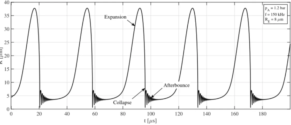
14
like thousands of degrees of Kelvin temperature or hundreds of bars of pressure around
15
the minimum radii of the bubbles [14]. Under these extreme conditions, even chemical
16
reactions start to take place. For instance, the dissociation of water and O2 molecules
17
produce H2 molecules, OH radicals or even oxygen and hydrogen atoms. Chemical reac-
18
tions generated by ultrasonic irradiation is called sonochemistry in the literature [15, 16].
19
It is worth noting that around the collapse phase, visible light emission was also observed
20
experimentally [17, 18]; this phenomenon is often called sonoluminescence and can be
21
explained by the ionization of several gas components [19–21].
22
These kinds of intense conditions can be exploited in several important sonochemical
23
applications by taking advantage of the production of the aforementioned substances.
24
In this sense, a bubble is often considered as a micron-sized chemical reactor where
25
several types of elements are generated. These can react with each other inside the
26
bubble or they can even leave the bubble and enter the liquid via diffusion. Inside the
27
liquid, they usually react with other dissolved components modifying the composition of
28
the liquid domain. In general, sonochemical behaviour is widely used in polymerization
29
[22, 23], nanosynthesis [24], disposing pollutants [25, 26], wastewater technologies [27]or
30
in sonodynamic therapy as a promising technology for cancer treatment [28–30].
31
Describing the dynamics of bubbles is certainly the most important aspect in acoustic
32
cavitation. It has been studied by numerous researchers both numerically and experi-
33
mentally in the last couple of decades [9, 31–33]. The exact behaviour of a certain bubble
34
is influenced by many different parameters such as liquid features, gas content, excita-
35
tion properties and many others [34, 35]. Depending on the current parameter values,
36
the oscillation of a bubble generally consists of three different phases: a rather slow ex-
37
pansion stage when the bubble grows and the internal pressure decreases; a much more
38
rapid collapse phase when the bubble suddenly shrinks and the pressure inside increases
39
significantly; and finally, an occasionally appearing afterbounce phase which is a con-
40
sequence of the highly non-linear nature of bubble dynamics. A typical bubble radius
41
vs. time curve as a function of time is presented in Fig. 1 under single frequency ultra-
42
sound excitation where the aforementioned phases are highlighted. An intense collapse
43
phase is expected in every sonochemical application [36]. Nevertheless, in some special
44
cases, other features may also become important, for instance chaotic oscillation [37] in
45
micromixing [38, 39].
46
There are plenty of studies that focus on describing the sonochemical behaviour of
47
bubbles; essentially they can be divided into two main groups. A smaller number of
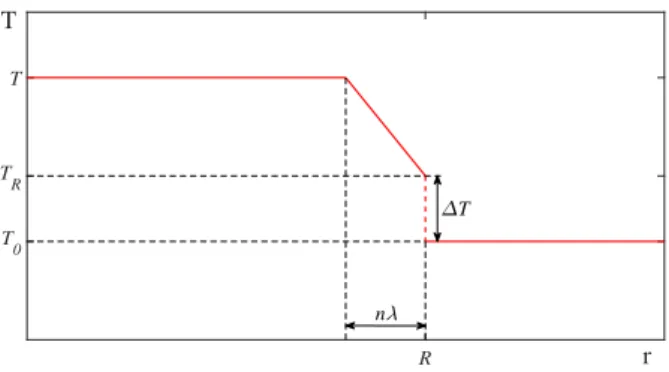
48
studies carry out simulations by taking into account the entire chemical modelling inside
49
the bubble [40, 41]. These models have a detailed and sophisticated implementation
50
of the bubble interior; thus, their complexity is significantly higher compared to the
51
classical Rayleigh approach [42]. Consequently, the numerical implementation can be
52
2
0 20 40 60 80 100 120 140 160 180 t [ s]
0 5 10 15 20 25 30 35 40
R [m]
Expansion
Collapse
Afterbounce
pA = 1.2 bar f = 150 kHz RE = 8 m
Figure 1: A typical bubble radius vs. time curve as a function of time under single frequency ultrasonic forcing. A relatively slow expansion phase is followed by a rapid collapse and some afterbounces.
a cumbersome task, especially when runtime is an important factor. The first aim of
53
the present paper is to implement a mathematical model, which is capable to describe the
54
chemical kinetics inside a bubble and to exploit the high processing power of professional
55
graphics cards (GPUs). Therefore, complex modelling and large parameter studies can
56
be achieved.
57
The other group of studies make conclusions only from the dynamical properties
58
of the bubbles without modelling the exact internal chemical processes. They define
59
various kinds of collapse strengths as an indicator for the chemical activity. Their obvious
60
advantage is that the model is quite simple and easy to implement; however, they suffer
61
from several general approximations. They state that the defined collapse strength is
62
strongly related to chemical activity [43]; moreover, it is declared that above a given
63
threshold of the collapse strength, the bubble is considered as chemically active. It is a
64
simple “binary” statement about the existence of chemical reactions; however, it can not
65
quantify the chemical output. By the best knowledge of the authors, the relationship
66
between the bubble dynamics and the chemical activity is poorly investigated in the
67
literature. The second purpose of the present study is to prove the existence of a clear
68
correlation between the chemical output and the dynamic features (collapse strength) of a
69
bubble by solving the detailed internal chemical processes numerically. Furthermore, we
70
aim to create mathematical formulae to characterise this relationship; thereby, propose
71
a “tool” that can estimate the chemical output only from the dynamical attributes of the
72
system (bubble radius vs. time curves).
73
The employed liquid is water saturated with pure oxygen. In our work, the control
74
parameters are the pressure amplitude and the frequency of the ultrasound, and the
75
bubble size. Changing the excitation parameters is the easiest way to influence bubble
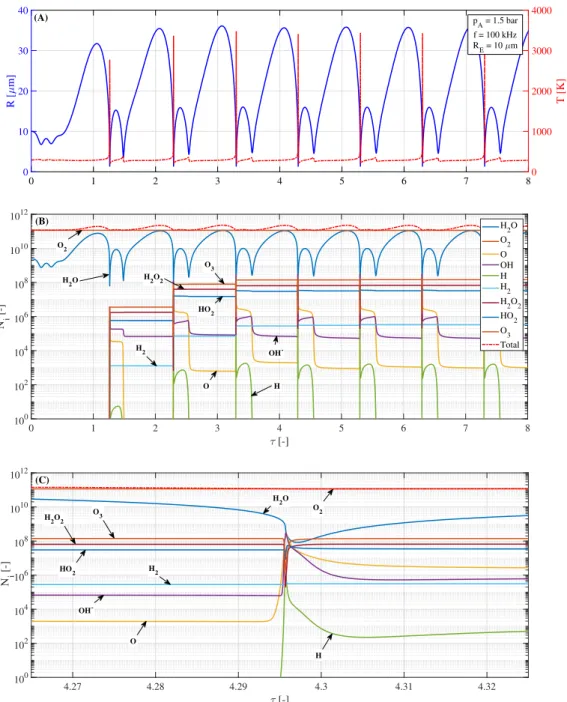
76
behaviour in an ultrasonic technology. Such a three-dimensional parameter space gives
77
a good overview of the behaviour of the system that can be used to find trends and
78
dependencies between different quantities.
79
2. The physical and the mathematical model
80
The physical model applied in the present study takes into account the following
81
effects. First of all, a single spherical bubble in water is examined in the presence of
82
harmonic pressure excitation. The bubble contains different types of non-condensible
83
gases (oxygen and various chemical products) and water vapour. Heat transfer, diffusion
84
into the liquid, evaporation and condensation of water, and reaction kinetics are included
85
in the model. The internal pressure and temperature is considered spatially uniform
86
except in a thin thermal boundary layer described later.
87
The radial dynamics of the bubble is described by the Keller–Miksis equation [44] in the form of
1− R˙ cL
!
RR¨+ 1− R˙ 3cL
!3 2
R˙2 = 1 + R˙ cL
+ R cL
d dt
!(pL−p∞(t)) ρL
, (1) whereR(t) is the radius of the bubble,tis the time,cL is the sound speed in the liquid andρL is the density of the liquid. The dots stand for derivatives with respect to time.
Note that the equation is of second order. The far field pressurep∞(t) consists of static and dynamic parts written as
p∞(t) =P∞+pAsin(2πf t), (2)
where P∞ is the static ambient pressure, pA and f are the pressure amplitude and frequency of the excitation, respectively. The liquid pressure pL at the bubble wall is related to the internal pressure as
p(t) =pL+2σ R + 4µL
R˙
R, (3)
wherep(t) is the internal pressure of the bubble,σis the surface tension and µL is the
88
dynamic viscosity of the liquid. It must be stressed that several researches [45–47] have
89
shown that at intense collapse regimes (when the bubble can grow up to ten times of
90
its equilibrium size) the bubble wall velocity can exceed the sound speed of the liquid.
91
This limits the validity range of our model. In this paper, however, we are focusing on
92
establishing model that describes the chemical model properly but still simple enough
93
to perform large parameter studies (approximately two million parameter combinations,
94
see Sec. 4). Thus this effect is neglected in the present study.
95
The internal pressure of the gas mixture is calculated via the van der Waals equation of state
p+an2 V2
(V −nb) =nRgT, (4)
whereaandbare the van der Waals constants of the mixture,nis the amount of the gas
96
mixture,V = 4R3π/3 is the volume of the bubble,Rg is the universal gas constant and
97
Tis the internal temperature. The van der Waals constants of the mixture are calculated
98
as
99
a=
C
P
i=1
Niai
Nt , (5)
4
b=
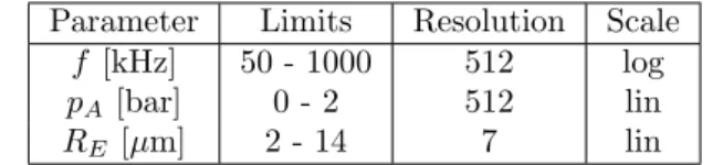
C
P
i=1
Nibi Nt
, (6)
where C is the number of the different chemical components in the bubble, Ni is the molecule number of componenti,Ntis the total molecule number,ai andbi are the van der Waals constants of component i. In order to calculate the internal pressure from Eq. (4), one has to determine the temperature inside the bubble. It is estimated from the internal energy of the mixture, which can be written as
E=
C
X
i=1
Nicv,i
! T NA
− Nt
NA
2
a
V, (7)
whereNA is the Avogadro-constant and cv,i is the molar heat capacity of componenti calculated by
cv,i= fi
2Rg, (8)
where fi is the degree of freedom of molecule i. For monoatomic gases, fi = 3; for
100
diatomic gases,fi = 5; and for gases of 3 or more atoms,fi = 6. The rate of change of
101
the internal energy will be described later in this section.
102
For the estimation of the heat transfer between the bubble and the liquid, the bubble
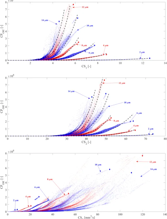
103
temperature (T) is assumed to be spatially uniform except in a thermal boundary layer
104
near the bubble wall in the internal side. In this layer, the temperature changes linearly
105
from the internal temperature of the bubble to the wall temperature (TR). Throughout
106
the manuscript,T represents the uniform part of the internal temperature that governs
107
the chemical processes. This approach of temperature distribution is a fairly simple model
108
for the internal temperature and thermal processes. Zhang et al. [48] made a detailed
109
research of the internal temperature and the internal pressure distributions. They have
110
shown that the temperature is the highest mostly at the bubble center and it decreases
111
drastically with the radial co-ordinate. Due to the reasons mentioned previously (large
112
number of parameter combination), a simplified approach is employed here to be able to
113
use a “non-distributed” computations of the chemical reactions.
114
At the bubble wall, a temperature jump occurs [49]:
∆T =− 1 2kn0
rπm 2kT
2−a0αe
αe
κ ∂T
∂r r=R
, (9)
where k is the Boltzmann-constant, n0 is the number density of the gas mixture, m is the average mass of a molecule inside the bubble,a0 and αe are constants [49],κis the average thermal conductivity of the mixture andris the radial coordinate. The liquid temperatureT0is assumed to be constant, thus, the internal temperature at the wall is TR=T0+ ∆T. The thickness of the thermal boundary layer is nλ, where nis constant andλis the mean free path of a molecule calculated as [50]
λ= V
√2σ0Nt, (10)
R r T
0 TR T T
n T
Figure 2: Sketch of the temperature distribution inside and outside the bubble. The internal temperature Tremains spatially uniform except for a thermal boundary layer, where the temperature changes linearly fromT toTR. A temperature jump (∆T) exists at the bubble wall.
whereσ0 is the average cross-section of the molecules. With this, the derivative of the temperature at the bubble wall became
∂T
∂r r=R
= TR−T
nλ . (11)
A schematic drawing about the temperature distribution is illustrated in Fig. 2.
115
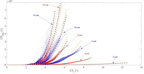
During the oscillation of a bubble, evaporation and condensation takes place due to the change of internal pressure and temperature. The rate of evaporation for unit area and time is [51, 52]
˙
meva= αM
√2πRv
p∗v
√T0
, (12)
where ˙mevais the rate of evaporation (in kg/m2s),αM is the accommodation coefficient for evaporation,Rv is the specific gas constant of water vapour and p∗v is the saturated pressure of vapour (atT0). The rate of condensation for unit area and time is calculated by the expression
˙
mcon= αM
√2πRv
Γpv
√T, (13)
where ˙mcon is the rate of condensation (in kg/m2s), Γ is the correction factor andpv is the actual partial pressure of the vapour inside the bubble, which is determined as
pv= NH2O Nt
p, (14)
whereNH2O is the number of vapor molecules inside the bubble. Now, the net rate of evaporation ˙mfor unit area and time can be expressed as
˙
m= ˙meva−m˙con. (15) The energy carried by an evaporating/condensing molecule is
eeva=cv,H2O
NA T0, (16)
6
econ= cv,H2O
NA TR, (17)
whereeevaandecon are the energy carried by an evaporating and condensing molecule,
116
respectively. It should be noted here that based on the measurements of Hickman [53]
117
and Maa [54], correction factor Γ was always chosen to be unity.
118
The diffusion into the liquid is modelled similarly to that of heat transport. The rate of diffusion for each component is determined by [40, 55]
dm dt
i
=
D ∂c
∂r r=R
i
≈Dc0,i−ci
ldiff , (18)
where (dm/dt)i is the rate of diffusion for component i (for unit area and time), D is the diffusion coefficient, c0,i is the concentration of component i at r = ∞, ci is the saturation concentration of componentiat the bubble wall in the liquid and ldiff is the diffusion length approximated by
ldiff= min
sRD
|R|˙ ,R π
!
. (19)
The saturation concentrationci is expressed by Henry’s law as ci= 103ρLNA
MH2OKBpi, (20)
whereKB is the Henry-constant in water and pi is the partial pressure of componenti inside the bubble calculated by Dalton’s law as
pi=Ni
Nt
p. (21)
The energy carried by a diffusing molecule is
ei=
cv,i
NATR, if dm
dt
i
<0, cv,i
NA
T0, if dm
dt
i
>0,
(22)
whereei is the energy carried by one diffusing molecule of componenti.
119
The chemical reactions taking place inside the bubble are estimated as follows. Let us consider the reaction
γ:A+B→C+D. (23)
Here,AandB are called reactants,C andD are called products. In each reaction, one molecule of each reactant is consumed and one molecule of each product is produced.
The rate of reactionγ is calculated by the modified Arrhenius-equation as
rγ =kγ[A][B] =AγTbγe−cγT [A][B], (24)
whererγis the rate of reactionγ,kγis the Arrhenius-coefficient of reactionγ, the brackets mean the concentration of the component. The quantitiesAγ, bγ and cγ are constants specific to reactionγ. The reaction rates relate to unit volume and unit time. Naturally, one component can take part in more than one chemical reactions. Consequently, the number of the molecules of a specific component changes due to every reactions it takes part in. As a result, the rate of change of the number of the molecules of a component is
N˙i =V X
(ri,prod−ri,destr) +A dm
dt
i
, (25)
whereri,prodandri,destrare the sum of every reaction rates where componentitakes place in as product and reactant, respectively. Here, A stands for the surface of the bubble, since diffusion into the liquid also affects the molecule number. Only the molecule number of vapour is treated differently as evaporation and condensation have to be taken into account:
N˙H2O=V X
(rH2O,prod−rH2O,destr) +Am.˙ (26) As it is mentioned before, the rate of change of the internal energy has to be deter- mined. It is calculated by the first law of thermodynamics:
E˙ =−pV˙ + ˙Q, (27)
where ˙Eis the rate of change of the internal energy and ˙Qis the sum of heats transferred into the bubble by each physical effect. Here, it is calculated by
Q˙ =A
C
X
i=1
dm dt
i
ei+κ ∂T
∂r r=R
+103NA MH2O
˙
mevaeeva−103NA MH2O
˙ mconecon
!
+V X
γ
(rγ,b−rγ,f)∆Hγ,f
! , (28) whereγ stands for every reactions taken into account. The indices f and b denote the
120
forward and backward reactions, respectively. ∆Hγ,f means the reaction heat of the
121
forward reaction. The first term in the first parentheses is the energy carried by diffusing
122
molecules, the second term is the thermal heat flux into the bubble. The third and fourth
123
terms are the energy carried by evaporating and condensing water molecules, respectively.
124
The second parenthesis stands for the heat change due to chemical reactions.
125
Finally, the overall ordinary differential equation (ODE) system that has to be solved
126
consists of the following equations: the Keller–Miksis-equation (1), the energy equation
127
(27) and the molecule number equations for all different chemical substances taken into
128
account by Eqs. (25) and (26). This results in an ODE system of C+ 3 equations,
129
where C is the number of different chemical species (the second order Keller–Miksis-
130
equation is solved as a first order system). During each ODE function evaluation, one
131
has to calculate the internal temperature and pressure from Eqs.(4) and (7), then the
132
different quantities in Eq. (28). This includes thermal conduction, evaporation, diffusion
133
and reaction kinetics.
134
The numerical method, that is applied here to solve the system is the Runge–Kutta–
Casp–Karp-method, which is a 4th-5th order explicit scheme with embedded error esti- mation. It must be stressed that from Eq. (4), expressing the derivative ofp, needed in
8
the Keller–Miksis equation, would become extremely complicated, therefore it is approx- imated linearly as
dp dt
j
≈pj−pj−1
tj−tj−1, (29)
where j relates to the current time step. Surely, an initial value of dp/dt has to be
135
specified for j = 0. In our calculations, the Keller–Miksis equation and the energy
136
equation is solved in dimensionless form, the process is described in Appendix A in
137
detail.
138
In the present work, we assumed initially pure O2and water vapour bubbles similarly
139
to the investigations by [56–58]. We considered altogether 9 different molecules and 44
140
different chemical reactions (22 reactions with their backward reactions as well). The
141
equations, theA, b, c and ∆Hf constants are given in Tab. 2 [59–61]. This results in an
142
ODE system of 9 + 3 = 12 equations.
143
The main purpose of the present study is to investigate the chemical production
144
of a driven bubble in the (f −pA) plane for various bubble sizes. In our survey, the
145
resolution of this parameter plane is 512×512 = 262144 with ranges ofpA∈[0,2] bar
146
(linear scale) and f ∈ [50,1000] kHz (logarithmic scale). The bubble size is described
147
by the equilibrium bubble radiusRE, that is the radius of the unexcited bubble. In our
148
simulations we examined 7 different sizes with the values of RE = 2,4,6,8,10,12 and
149
14µm. Thus, the total number of the investigated parameter combinations are 1835008.
150
Every other parameters are fixed, their values are shown in Tab. 1.
151
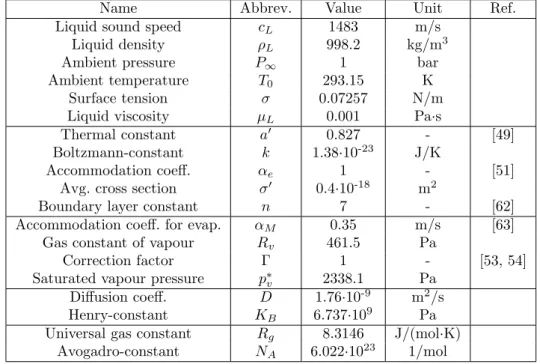
Table 1: The parameters kept constant during the simulations. The references for some non-trivial values are indicated.
Name Abbrev. Value Unit Ref.
Liquid sound speed cL 1483 m/s
Liquid density ρL 998.2 kg/m3
Ambient pressure P∞ 1 bar
Ambient temperature T0 293.15 K
Surface tension σ 0.07257 N/m
Liquid viscosity µL 0.001 Pa·s
Thermal constant a0 0.827 - [49]
Boltzmann-constant k 1.38·10-23 J/K
Accommodation coeff. αe 1 - [51]
Avg. cross section σ0 0.4·10-18 m2
Boundary layer constant n 7 - [62]
Accommodation coeff. for evap. αM 0.35 m/s [63]
Gas constant of vapour Rv 461.5 Pa
Correction factor Γ 1 - [53, 54]
Saturated vapour pressure p∗v 2338.1 Pa
Diffusion coeff. D 1.76·10-9 m2/s
Henry-constant KB 6.737·109 Pa
Universal gas constant Rg 8.3146 J/(mol·K) Avogadro-constant NA 6.022·1023 1/mol
Table 2: The applied chemical reactions in the model [59–61]. The indicesfandbrefer to the forward and backward reactions, respectively. The unit ofcis K,bis dimensionless and ∆Hf is in kJ/mol. The units ofAis m3/(mol·s) for two-body reactions and m6/(mol2·s) for three-body reactions (see Eq. (24) for details).M denotes third body that does not take part in the reaction itself.
Reaction Forward Backward
∆Hf
Af bf cf Ab bb cb
H2O+M→OH+H+M 1.96·1016 -1.62 59700 2.25·1010 -2 0 508.82 O2+M→O+O+M 1.58·1011 -0.5 59472 6.17·103 -0.5 0 505.4 H2O+O→OH+OH 2.21·103 1.4 8368 2.1·102 1.4 200 72.59 OH+H→O+H2 2.64·10-2 2.65 2245 5.08·10-2 2.67 3166 8.23
OH+M→O+H+M 4.72·106 -1 0 4.66·1011 -0.65 51200 436.23
H2O+OH→H2O2+H 1.41·105 0.66 12320 4.82·107 0 4000 64.32 HO2+OH→H2O2+O 4.62·10-3 2.75 9277 9.55 2 2000 56.06
O+O2+M→O3+M 4.1 0 -1057 2.48·108 0 11430 -109.27
OH+O2→O3+H 4.4·10 1.44 38600 2.3·105 0.75 0 96.2
H+O3→O+HO2 9.0·106 0.5 2010 0 0 0 135.65 OH+OH+M→H2O2+M 9.0·10-1 0.9 -3050 1.2·1011 0 22900 217.89 HO2+H→OH+OH 1.69·108 0 440 1.08·105 0.61 18230 -162.26 HO2+O→OH+O2 1.81·107 0 -200 3.1·106 0.26 26083 231.77 H2O+HO2→H2O2+OH 2.8·107 0 16500 1.0·107 0 900 -128.62 O2+O2→O3+O 1.2·107 0 49800 5.2·106 0 2090 396.0 H2+HO2→H2O2+H 1.41·105 0.66 12320 4.82·107 0 4000 64.32
O+OH→H+O2 7.18·105 0.36 -342 1.92·108 0 8270 69.17
OH+H2→H+H2O 2.18·102 1.51 1726 1.02·103 1.51 9370 64.35 OH+HO2→H2O+O2 1.45·1010 -1 0 2.18·1010 -0.72 34813 -304.33
H+O2+M→HO2+M 2.0·103 0 -500 2.46·109 0 24300 204.8 HO2+H→H2+O2 6.63·107 0 1070 2.19·107 0.28 28390 239.67 H2+M→H+H+M 4.58·1013 -1.4 52500 2.45·108 -1.78 480 444.47
The initial conditions of the simulations are as follows. The bubble was always initi- ated from equilibrium state, thusR(0) =RE and ˙R(0) = 0. The corresponding equilib- rium pressure is
pE =P∞+ 2σ
RE. (30)
Similarly, the initial value for the pressure derivative in Eq. (29) is 0. In the beginning, we assumed only O2 and vapour molecules inside, with the partial pressure of vapour being the saturated vapour pressure (p∗v) at ambient temperature. This yields the partial pressure of O2to bepO2,0=pE−p∗v. Here, the index 0 denotes the initial value. Assuming ideal gas, the initial number for oxygen is
NO2,0=pO2,0
V0NA
RgT0
, (31)
and for vapour, it is
NH2O,0= p∗v pO2,0
NO2,0. (32)
10
Finally, the energy that belongs to equilibrium state is EE= T0
NA X
i
Ni,0cvi,0− Nt,0
NA 2a0
V0. (33)
In the case of diffusion, we assumed that the liquid has only dissolved O2 [64] and that the saturated O2concentration is 10% of the initial concentration inside the bubble. This yields
c0,O2 = 103ρLNA MO2KB
NO2,0 Nt,0
p0·0.1. (34)
Concentration of every other chemical substances in the liquid is supposed to be 0.
152
Due to the high number of parameters and the complexity of our system, the numer-
153
ical solving process can be extremely slow. In order to accomplish the above described
154
tasks, we decided to employ High Performance Computing (HPC) by utilizing the mas-
155
sively parallel architecture of Graphic Processing Units (GPUs). They have high amount
156
of computational performance and cheap prize relative to that of CPUs. GPUs have
157
thousands of parallel computational units that can work simultaneously; thus, they are
158
suitable for making high resolution parameter studies, which is the main goal here. How-
159
ever, the biggest difficulty of using GPUs is that the user needs deep knowledge of the
160
hardware architecture in order to write an efficient code and fully utilise the processing
161
units. For detailed description of GPU programming to solve large number of indepen-
162
dent ODE systems, the reader is referred to publications [65, 66]. The calculations are
163
performed on an NVIDIA GeForce GTX Titan Black graphics card having a peak double
164
precision processing power of 1707 GFLOPS.
165
3. The chemical output and the collapse strength of a bubble
166
Initiating a given system from the aforementioned initial conditions and performing
167
the simulation for a given time, one can obtain the time curves of the bubble radius, wall
168
velocity, internal energy and molecule numbers of each chemical species.
169
Figure 3 shows the results atf = 100 kHz, pA= 1.5 bar and atRE= 10µm for the
170
first 8 excitation cycles (the time axes are always in dimensionless formτ =t·f, thus
171
τ = 1 relates to one excitation period). On chart (A), the time curves of the bubble
172
radius (blue line) and the temperature (red dotted line) are displayed. The first collapse
173
stage starts slightly afterτ= 1, at aroundτ = 1.2, where the temperature grows above
174
3000 K. This high temperature indicates the presence of the reactions that dissociate
175
H2O molecules. Their products also start to be produced (e.g. H2O2, OH- or H2, see the
176
complete list of molecule numbers on chart (B)). In the expansion phase, the number
177
of the vapour molecules tends to grow by two orders of magnitude as a result of high
178
amount of net evaporation rate from the liquid due to the low internal pressure. In the
179
collapse phase, most of the vapour molecules dissociate and the molecule numbers of
180
the other products start to increase rapidly. It can be observed from chart (B) that in
181
the first couple of collapses (around 3 or 4), the molecule numbers of the products grow
182
gradually until they saturate at a given level. For instance, the molecule number of H2
183
(light blue line) is 0, 103, 7·104and 2·105 during the first 4 acoustic cycles, respectively.
184
After this initial transient phase, all molecule numbers — except vapour and H atom —
185
0 1 2 3 4 5 6 7 8 0
10 20 30 40
R [m]
0 1000 2000 3000 4000
T [K]
(A) p
A = 1.5 bar f = 100 kHz RE = 10 m
0 1 2 3 4 5 6 7 8
[-]
100 102 104 106 108 1010 1012
Ni [-]
H2O O2 O OH H H2 H2O
2 HO2 O3 Total O3
O
OH- H2
H H2O
O2
H2O2
HO2
(B)
4.27 4.28 4.29 4.3 4.31 4.32
[-]
100 102 104 106 108 1010 1012
N i [-]
O2
H OH-
H2 HO2
H2O H2O2 O3
O
(C)
Figure 3: Bubble radius (blue line), temperature (red line) on chart (A) and molecule numbers on chart (B) withpA = 1.5 bar,f = 100 kHz andRE = 10µm, in the first 8 acoustic cycles. A detailed view around the strong collapse is shown on chart (C).
12
stay constant in the expansion phase after the small afterbounces. This means that the
186
net production rate becomes nearly zero as these products tend to dissociate on lower
187
temperatures.
188
Although it is hard to identify from the time curves, diffusion into the liquid always
189
presents, meaning that a certain amount of molecules are continuously leaving the bubble.
190
Eventually, this could result in an overall decrease of the number of the molecules inside
191
the bubble, but the evaporating vapour molecules always tend to “replace” this loss.
192
Therefore, this procedure keeps diffusion of the chemical species into the liquid domain
193
a rather constant process maintaining a dynamical equilibrium. It must be emphasized
194
that the time scale of the diffusion process is orders of magnitudes higher than that of
195
the characteristic time scale of the radial dynamics of the bubble. This phenomenon
196
has a severe consequence. During the initial transient (see Fig. 3), the production of the
197
chemical species is high, their concentration increases rapidly inside the bubble. However,
198
after the initial transients (few cycles), the concentration of the species saturates at
199
a certain level and the net production rate becomes nearly zero. The existence of a
200
small positive production rate is due to the slowly diffusing molecules into the liquid
201
domain. This is the reason why Mettin et al. [16] observed orders of magnitude higher
202
sonochemical output when the acoustically driven bubble was spherically unstable. In
203
their case, during the non-spherical collapse phase, the produced chemical components
204
are released into the liquid also via a complex mixing procedure besides the slow diffusion
205
process. Nevertheless, the present paper assumes spherical stability and focuses only on
206
the released chemical species by diffusion.
207
On chart (C), an enlarged view around the fourth strong collapse of chart (B) is
208
presented. It can be observed that the number of the molecules of vapour drops signifi-
209
cantly here due to the high rate of dissociation of H2O. Similarly, the production of e.g.
210
H atom, OH- or O atom increase drastically in the collapse phase. In the forthcoming,
211
much slower, expansion phase, the amount of these types of molecules tend to decrease
212
considerably keeping the dynamical equilibrium. However, some substances (e.g. O3,
213
HO2, H2O2) are reduced in the collapse phase but they are regained in the expansion
214
phase. In general, Fig. 3 suggests that the production of chemical species are gener-
215
ally caused by the dissociation of H2O; the O2 molecules are mainly stay at a constant
216
amount. This implies that it is the amount of vapour that influences chemical output
217
rather than the initial gas content (pure oxygen here).
218
In order to connect the chemical activity of the bubble to its radial dynamics, proper characterisation of the collapse strength of a bubble is required. In the literature, the strength of the collapse is usually quantified by the following formulae [67–69]:
CS1=Rmax−RE
RE
(35)
CS2=Rmax
Rmin
(36)
CS3= Rmax3
tc , (37)
whereCS refers to collapse strength, Rmax is the maximum value ofR(t),Rmin is the
219
subsequent minimum value ofR(t) andtc is the collapse time, which is the elapsed time
220
between the maximum and minimum values ofR(t). In the literature,CS1 andCS2 is
221
referred to as relative expansion and compression ratio, respectively. Observe that all
222
these three quantities are derived only from the R(t) curve; therefore, they represent
223
the dynamical nature of the system around the collapse phase. It is commonly accepted
224
[43, 70] that the threshold for sonochemical activity isCS1= 2; however, the relationship
225
between the chemical output and the magnitude of the above defined collapse strength
226
is rarely investigated.
227
As we assume spherical stability, we define the chemical production as the number of diffusing molecules into the liquid during one acoustic cycle as an average of 10 cycles.
It is written mathematically as CPi= 1
10 Z 10T
0
A dm
dt
i
dt, (38)
where T = 1/f is the period of the excitation, A stands for the surface area of the
228
bubble andCPimeans the chemical production of componenti. It is clear that chemical
229
production can be constructed for all types of diffusing species. The higher the chemical
230
production of certain substances, the better the sonochemical output of the stable bubble
231
for a given application. It depends on the specific application which chemical product
232
is useful in a process; that is, maximizing the chemical production of certain species is
233
keen interest of sonochemistry.
234
It is emphasized here that in our calculations, every simulation is run up to 30 periods
235
of excitation, hence the effects of aforementioned initial transients could be neglected.
236
Consequently, chemical production is estimated for the last 10 acoustic cycles, and the
237
necessary quantities for collapse strengths (Rmax, Rmin, tc) are determined from the last
238
cycle.
239
4. The global overview of the chemical output in the 3D parameter space
240
High resolution numerical simulations are performed on the excitation amplitude -
241
excitation frequency (pA−f) parameter plane at different bubble sizes RE. The exact
242
values of these control parameters are given in Tab. 3. Again, the total number of the
243
parameter combination is 512×512×7 = 1835008. For the details of the simulation set
244
up at every parameter set, see the detailed description of the previous section.
245
Table 3: The control parameters, their resolutions and their scales.
Parameter Limits Resolution Scale
f [kHz] 50 - 1000 512 log
pA [bar] 0 - 2 512 lin
RE [µm] 2 - 14 7 lin
After each simulation, one can calculate the values of the different collapse strengths
246
CSi and the chemical production of every substance CPi using Eqs. (35)-(38). The
247
strategy is to create a series of high resolution bi-parametric plots over the pA −f
248
parameter plane at different values ofRE. Fig. 4 summarises the chemical productions of
249
OH-radical, H2O2, H2and O3for two different sizes (RE= 6 and 12µm). The frequency
250
14
and the chemical production are on logarithmic scale. The black lines denote several
251
iso-lines of the relative expansion CS1. From all charts of Fig. 4, it can be concluded
252
that chemical production rates grows quickly with increasing pressure amplitudepAand
253
with decreasing the frequency f for every substances. However, employing a constant
254
pressure amplitude, some peaks in the chemical production can be found at several values
255
of the frequency due to the harmonic resonances of the system [71–73] (for example
256
on chart (B), at pA = 1.5 bar, local maxima of chemical production can be noticed at
257
f ≈75 kHz and atf ≈138 kHz, marked by red squares). It can be observed that lowering
258
the bubble size makes these resonances denser, compare for instance charts (C) and (D).
259
On chart (C), at RE = 6µm, there are around 6 resonances in contrast to chart (D)
260
where there are only 3. It should be noted here that the trends of chemical production
261
are qualitatively the same for every chemical species. Thus, from now on, we only discuss
262
the case of the production of OH- radicals as the other components behave in a similar
263
way.
264
The most importantaspect in Fig. 4 is that the iso-lines ofCS1 correlate quite well
265
with the chemical production. This observation suggests that a clear relationship exists
266
between the collapse strength and the chemical production. In order to reveal the nature
267
of this dependence, at every parameter combination, the values of the collapse strength
268
CSi and the values of the corresponding chemical production CPi are collected in a
269
single diagram. Figure 5 demonstrates this condensed representation where the chemical
270
production of OH-radical is plotted as a function of the three different collapse strengths.
271
It is apparent that,particularly on Figs. 5A and B (CS1andCS2), the points related to
272
a specific bubble sizeshowa clear trend. Especially on smaller equilibrium radii (up to
273
approx. 8µm), the dependence is clear. However, over 10µm, the points gradually start
274
to exhibit scattered behaviour. Nevertheless, an obvious trend can still be visible. In the
275
case ofCS3, a clear trend between the collapse strength and the chemical output is hard
276
to be recognised compared to those ofCS1 and CS2. Due to such a poor correlation,
277
the further discussion ofCS3is omitted from now on.
278
From Fig. 5, it can be stated that the incidence of the chemical processes is approxi-
279
mately betweenCS1≈2−3. However, the exact value is less clear for smaller bubbles.
280
This confirms the typically accepted rule-of-thumb in the literature (e.g. [43]) that the
281
chemical reactions occur approximately over the value ofCS1≈2. Nevertheless, such a
282
threshold value does not provide information about the actual reaction rates. Observe
283
that atRE = 2µm, the chemical production of OH-remains relatively low as it does not
284
exceed 3·107molecules/cycle with a value of 12 forCS1. In contrast, the highest chemical
285
production occurs at aroundRE= 12µm of bubble size with a collapse strength of only
286
CS1 ≈6. This is due to the fact that a larger bubble can contain more molecules; that
287
is, larger reactive volume means higher total production. Moreover, a larger bubble has
288
obviously bigger surface, thereby increasing diffusion rate as well (see Eq. (38)) . As a
289
consequence, the collapse strength alone cannot determine the sonochemical production
290
quantitatively, the effect of the bubble size has to be included in such a description. This
291
is the main topic of the next section.
292
Figure 4: Bi-parametric plots of chemical productions of OH-radical, H2O2, H2and O3at two different bubble sizes (RE = 6 and 12µm). The black lines are the iso-lines of relative expansionCS1 for some
specific values. 16
Figure 5: Chemical production of OH-as a function of the three different collapse strengths. The values ofREare denoted by the arrows. The black dashed lines belong to the fitted curves via Eq. (39).
0 5 10 15 0
1 2
3 104 CS
1 = 13600 (erf[0.345(R
E - 6.4)] + 1)
0 5 10 15
RE [ m]
0 2 4 6 8 10
0 5 10 15
0 1 2 3
CS2
0 5 10 15
RE [ m]
0 2 4 6 8 10
R2 = 0.989
= 0.1499 R E + 4.098 R2 = 0.9475
(B)
(D) (C)
(A)
Figure 6: The values of parametersαandβforCS1andCS2, as a function ofRE. In the case ofCS1, the fitted curves are also indicated together with the corresponding equations as well.
5. Mathematical description of the chemical production as a function of the
293
collapse strength
294
As a final step, we aim to construct a mathematical formula between the collapse
295
strength and the sonochemical production. With the least squares method, we fitted
296
curves of the form
297
CP =α·CSiβ
(39) to the (CSi, CP) points. Hereαandβ are the fitting parameters. The fitted curves are
298
shown in Fig. 5 with the black dashed lines. The curves go through the (CS, CP) points
299
sufficiently well (theR2values are above 0.9 for every values ofRE). The exact values of
300
the fitting parameters forCS1andCS2as a function ofREare shown in Fig. 6 (αandβ
301
are in the first and second rows, respectively). For the case ofCS2, the values ofαandβ
302
do not follow an exact trend. ForCS1, on the other hand, it seems that the parameters
303
have a clear dependence on the equilibrium radius. In the following, we focus only on
304
CS1 as it has the best visible correlation between collapse strengthCS and the chemical
305
productionCP and it has the most clear trend in the fitted parameters as a function of
306
the bubble sizeRE.
307
From a viewpoint of applications and simplicity, it could be really useful if one can estimate the chemical activity and the production only from the dynamical properties of the bubble dynamics; for instance, only fromCS1. Therefore, we aimed to construct a rather simple mathematical formula, that can help to predict the sonochemical produc- tion of a single bubble using only the collapse strengthCS1 without the simulation of
18
the complex chemical system. The fitted curves to the values ofαandβ as a function ofRE, which are also presented in Figs. 6A and C are
α(RE) = 13600·(erf[0.345(RE−6.4)] + 1) (40) and
β(RE) = 0.1499·RE+ 4.098. (41)
Here, the functionerf(x) stands for the error function, which is defined by [74]
erf(x) = 2 π
Z x 0
e−t2dt. (42)
TheR2values of the two fits are 0.989 and 0.9475 forα(RE) andβ(RE), respectively. It
308
should be noted thatREhas to be inµm in Eqs. (40)) and (41). For the approximation of
309
α(RE), we intended to use a formula that tends to zero with decreasingRE, and saturates
310
with increasing RE while it is still a reasonable good fit. We are aware of the fact
311
that there is no specific physical meaning of the error function used here. Substituting
312
the RE values into Eqs. (40) and (41), then applying the results to approximate the
313
chemical production via Eq. (39), one can get slightly different curves compared to the
314
ones obtained by the individual fitting ofαandβ. This difference is shown in Fig. 7 where
315
the black dashed lines are the curves fitted independently to the points corresponding to
316
the different values ofRE, while the orange dashed lines is the ones obtained by using
317
the approximated coefficientsαandβ calculated from Eqs. (40) and (41). The difference
318
is not negligible; however, the orange lines also go through sufficiently well between the
319
(CS-CP) points. Thus they are quite good approximations to estimate the chemical
320
production of a single bubble.
321
Figure 7: The difference between the two kind of fitted curves: individually fittedαandβ(black curves);
and approximatedαandβfrom Eqs. (40) and (41) (yellow curves).
Figure 8: Values ofCP1estimated from the Keller–Miksis model as a function of those of the full chemical model on the same parameter regime (see Table 3.). The bubble sizes areRE = 4,6,10 and 12µm, respectively. The points are located fairly well around a straight line with the slope of 45 degrees (denoted with black lines).
By employing Eqs. (39)-(41), it becomes possible to estimate the chemical production
322
of the system without explicitly calculating the chemical reactions. It is a remarkable
323
result, because by solving the Keller–Miksis equation, the dynamics of a single bubble is
324
relatively simple to calculate and it is the widely applied method in the investigation of
325
bubble dynamics. This can be helpful during the optimisation of sonochemical reactors.
326
For validating this kind of application, it has to be proven that the values of collapse
327
strengthCS1 are approximately the same with both the full-model (including chemical
328
kinetics) and the sole Keller–Miksis equation (without chemical reactions). Therefore,
329
we repeated the simulations on the parameter regime shown in Tab. 3 using only the
330
Keller–Miksis equation (Eqs. (1)-(3)). The two type of collapse strengths are presented
331
as a function of each other in Fig. 8 for four different bubble sizes. It can be clearly seen
332
that the points are located around a straight line with a slope of 45 degrees. This implies
333
that the values of the collapse strengths are approximately the same for both models.
334
Thus, no correction is necessary during the estimation of the chemical yield from the
335
bubble radius vs. time curves using the simple Keller–Miksis equation.
336
It should be emphasised, however, that the conclusions made above are based on many
337
assumptions/simplifications: e.g. uniform bubble interior, spherical stability, simplified
338
diffusion modelling and the approximations via curve fitting. Nevertheless, we believe
339
20
![Table 2: The applied chemical reactions in the model [59–61]. The indices f and b refer to the forward and backward reactions, respectively](https://thumb-eu.123doks.com/thumbv2/9dokorg/793587.37360/10.892.154.767.281.718/applied-chemical-reactions-indices-forward-backward-reactions-respectively.webp)