Structuralanalysisofbiochemicallymotivatednonlinearsystems PázmányPéterCatholicUniversity

(1)

P´ azm´ any P´ eter Catholic University

Doctoral Thesis

Structural analysis of biochemically motivated nonlinear systems

Author:

BernadettAcs´

Thesis Advisor:

Dr. G´abor Szederk´enyi, D.Sc.

A thesis submitted in partial fulfilment of the requirements for the degree of Doctor of Philosophy

in the

Roska Tam´as Doctoral School of Sciences and Technology Faculty of Information Technology and Bionics

2018

(2)

(3)

Abstract

Kinetic systems form a special class among nonnegative dynamical systems that are suitable to describe all kinds of dynamical behaviour. Kinetic systems can be applied for modelling various kinds of systems, such as biochemical reaction networks, electronic networks, transportation problems or the spreading of epidemics. The aim of this thesis is to study the structural properties of mass action kinetic systems and introduce novel algorithms for the computation of their realizations. During the computations the linear programming optimization framework is applied. It is proven that the dense linearly conjugate realization of a kinetic system with a fixed set of complexes and also fulfilling a finite set of additional linear constraints has the superstructure property. This plays an essential part in the presented methods. A polynomial-time algorithm is given for computing the dense linearly conjugate realization of a kinetic system that is significantly more efficient than the previously known methods. An already existing algorithm for determining a weakly reversible dynamically equivalent realization of a kinetic system is extended to the case of linearly conjugate realizations. Two methods are presented for computing all possible reaction graph structures representing linearly conjugate – and as special case dynamically equivalent – realizations of a kinetic system. Both methods are suitable for parallel implementation. A generalized form of kinetic systems is introduced that allows uncertain parameters and additional linear constraints as well.

The methods for computing a dense realization, the set of core reactions and all possible reaction graph structures are extended to this model as well. The correctness of each presented algorithm is proven, and their working is demonstrated on several examples.

(4)

Acknowledgements

First of all, I would like to thank my thesis advisor Prof. G´abor Szederk´enyi for intro- ducing me into this interesting topic and guiding me through its various and details by always giving me such problems that I was actually able to solve. I am also very grateful for his patience and understanding during our work together.

I would like to thank Prof. Zsolt Tuza for the opportunity of working with him. He has shown us some of his beautiful ideas, and beside that he has improved the presentation of our results considering even the smallest details, from which I have learnt a great deal.

I am thankful for the collaboration with former and present members of our group, especially to Dr. Zolt´an A. Tuza, Dr. D´avid Csercsik and Gergely Szlobodnyik for designing implementations for the algorithms introduced in this thesis. Without their work these would remain only theoretical results.

I am grateful to Prof. Katalin M. Hangos for the chance of taking part in and in some cases even delivering talks on seminars organized by her group at SZTAKI. It was not just a great opportunity for observing and participating, but her comments have also made a great impact on my documents as well as my presentation skills.

I would also like to thank Dr. J´anos T´oth for inviting me to seminars organized by him at BME. It was a great opportunity to present our results as well as to meet interesting people and new ideas.

I am really thankful to Dr. Ágnes Bércesné Novák for encouraging me to apply to the doctoral school. She has opened up new perspectives to me.

I am also very thankful to my family for their patience and support in various fields of life during the last four years.

I am grateful to the Roska Tam´as Doctoral School for accepting and supporting me during my road to graduation. I would like to specially thank Tivadarn´e Vida for kindly giving me all the help with administrative problems.

I would also like to acknowledge the support of the grants OTKA 104706, KAP 1.1 14/029, 1.1 15/052, 16-71005-1.1 and 17-61008-1.2. The doctoral school was also sup- ported by the European Union, co-financed by the European Social Fund (EFOP-3.6.3- VEKOP-16-2017-00002).

iii

(5)

Notations and Symbols

R the set of real numbers

R+ the set of nonnegative real numbers N the set of natural numbers, including 0 Rⁿ then-dimensional Euclidean space Rⁿ+ the nonnegative orthant in Rⁿ

|H| the number of elements in the setH

H^n×m the set of matrices having entries from a set H withnrows and m columns [M]ij the entry of a matrix M with row index iand column indexj

[M]_.j the column j of a matrixM

vec(M) the concatenation of the columns of the matrixM vec(M) = [[M]^>_.1, . . . ,[M]^>_.m]^>

eⁿ_i theith unit vector in Rⁿ, where

the coordinate iis equal to 1 and all other coordinates are zero 0ⁿ the zero vector inRⁿ

1ⁿ the vector in Rⁿ with all coordinates equal to 1 0^n×m the zero matrix inR^n×m

Iⁿ the unit matrix inR^n×n

0q the binary sequence of lengthq with all coordinates equal to zero 1q the binary sequence of lengthq with all coordinates equal to 1 sgn(x) the sign function

S the set of species of a CRN C the set of complexes of a CRN R the set of reactions of a CRN

Ci→Cj the reaction from complex Ci to complexCj

(C_i, C_j) the reference of reactionC_i →C_j in formulas k_ij reaction rate coefficient of the reaction C_i →C_j M the coefficient matrix of a polynomial system Y the complex composition matrix of a CRN A_k the Kirchhoff matrix of a CRN

ψ^Y(x) the monomial function of the CRN (Y, A_k) (independent from A_k) T positive definite diagonal transformation matrix

ΦT the transformation matrix of the monomial functionϕ [ΦT]ii=ϕi(T ·1^p)

Ψ_T the transformation matrix of the monomial functionψ_Y of the CRN (Y, A_k) [ΨT]ii=ψ^Y_i (T·1^m)

vi

(8)

Notations vii Ab the transformed Kirchhoff matrix of a linearly conjugate realization

A_b =A_k·Ψ⁻¹_T

[M, Y] the kinetic system defined by the coefficient matrix M and the complex composition matrix Y

[P, L, Y] the uncertain kinetic system defined by the polyhedronP

of uncertain parameters, the set Lof additional linear constraints and the complex composition matrix Y

(Y, A_k) the CRN characterized by the matrices Y andA_k

(T⁻¹, Ab) the linearly conjugate realization defined by the matrices T⁻¹ and Ab

Q the polyhedron representing the solutions of an optimization model Q the closure of the polyhedronQ

Ec[M, Y] the set of core edges of the kinetic system [M, Y] G(Y, A_k) the reaction graph of the CRN (Y, A_k)

V(G) the set of vertices of the graph G E(G) the set of edges of the graphG

K_m complete directed graph onm vertices

R a realization and its representation as a binary sequence

D the dense realization and its representation as a binary sequence G_R the reaction graph structure of the realization R

e(R) the number of edges of the graph GR

(9)

Chapter 1

Introduction

The development and/or the maintenance of any kind of device or system requires some kind of knowledge about its possible states. To reveal the connections among properties of different events and to try to predict certain characteristics of the future quantitative mathematical models are successfully applied. These models usually describe only se- lected properties of the real process, but from an application point of view in most cases it is enough.

The operation of more complicated systems such as living organisms can often be described by complex phenomena, and for the modelling of quantities changing in space and/or in time dynamical systems are the most commonly applied tools. Therefore, this type of modelling has become an intensively studied and frequently applied tool in systems biology.

In many real life problems for example in economic systems, population dynamics or biochemical systems the variables are physically constrained to have only nonnegative values, and therefore the theory of nonnegative systems [1] needs to be applied for their characterization. A dynamical system is called nonnegative if its trajectories remain in the nonnegative orthant whenever the initial value is nonnegative. (If strict positivity is required then it is called a positive system.) A wide subclass of dynamical systems can be transformed into nonnegative form by shifting the coordinates into the nonnegative orthant and then in a further transformed version of the model the trajectories can be kept in a given region, see [2].

A more special class of nonnegative dynamical systems is formed by the quasi polynomial (QP) systems, which was first introduced in [3]. The author has also shown that most smooth dynamical models can algorithmically be transformed into QP form, which property makes such systems suitable for the modelling of dynamical systems belonging to a much wider class.

If the right hand side of the ordinary differential equations of the system can be given in the form of a multivariate polynomial as well, then it is called a polynomial system.

The aim of this thesis is the structural and computational analysis of a certain type of nonnegative polynomial systems called kinetic systems, that can describe the dynamics

1

(10)

Chapter 1. Introduction 2 of chemical reaction network (CRN) models obeying the mass action law. Despite the fact that kinetic systems are rather special polynomial systems, these models are versatile tools in modelling. Furthermore, by using suitable model transformations the majority of nonnegative dynamical systems can be transformed into kinetic form [3, 4].

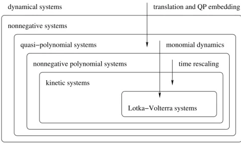
The different types of dynamical systems and possible transformations between them are shown on the diagram in Figure 1.1. It has to be mentioned however, that the examination of model types different from kinetic systems and of the transformations between these models is not included in this thesis.

quasi−polynomial systems

nonnegative polynomial systems nonnegative systems

kinetic systems

time rescaling

Lotka−Volterra systems

monomial dynamics translation and QP embedding dynamical systems

Figure 1.1: Classes and transformations of dynamic systems.

Chemical reaction networks obeying the mass action law can be originated from the dynamical modelling of chemical and biochemical processes, but they can be applied to describe various kinds of dynamical phenomena. Their applications appear in several different fields of science and engineering, such as the modelling of electrical networks, transportation problems or the spreading of epidemics, therefore these models are so- called universal descriptors [5,2].

The class of kinetic systems is defined by chemical reaction network models, but for the verification of the kinetic property it is not necessary to compute a suitable CRN, it is enough to examine just the sign pattern of the monomial coefficients, see [6].

It is known that in general there are many realizations and different reaction graph structures corresponding to a given kinetic dynamics. This phenomenon is called macro- equivalence or dynamical equivalence [7,8]. There is also a generalization of dynamical equivalence called linear conjugacy, where a positive definite diagonal linear transformation is applied to the state variables working as if the units of measurement were individually scaled [9]. It is easy to see that linear conjugacy preserves the kinetic property of the system and also the main qualitative dynamical properties like stability, multiplicities or the boundedness of solutions. However, due to the larger degree of

(11)

Chapter 1. Introduction 3 freedom introduced by the transformation parameters, in general, it allows a larger set of possible structures compared to dynamical equivalence.

There is a widely applied structure oriented representation of CRNs that is a weighted directed graph called the Feinberg-Horn-Jackson graph. It depicts the reactions which are present in the network, and some other parameters of the network as well that are easier to describe with graph properties. Furthermore, in some cases there is a relation between the dynamics of the network and the reaction graph structure, without considering the actual reaction rates. This has become an important research area in chemical reaction network theory since the 1970s, see [7, 10]. In this topic there are several practice oriented results [11] as well as beautiful mathematical designs [12].

To determine a possible reaction network structure of a given kinetic system a symbolic method was proposed in [6]. Since this method returns only one particular dynamically equivalent realization called the canonical realization, a different approach must be applied to determine others.

Chemical reaction networks have a simple algebraic characterization, which makes it particularly appealing to develop computational methods for their dynamical and structural analysis [13, 1] or even control [14]. Realizations of a given kinetic dynamics can be defined by linear constraints, that suggests the application of linear optimization methods. Since this is in general a very simple model, several computational methods have already been developed to find linearly conjugate or, as a special case, dynamically equivalent realizations of kinetic systems [15, 16] and also having preferred properties such as density/sparsity [17,18], maximal or minimal realizations [19], complex or de- tailed balance [20,21], weak reversibility [22], [51] or minimum deficiency [23,24].

The general form of these problems can be written as a linear programming (LP) model using only continuous decision variables. For solving an LP problem there are several polynomial time algorithms, the first provably correct solution is the Simplex Algorithm that was developed by Dantzig in 1947 [25, 26]. This algorithm works in most of the practical applications very efficiently, however in 1972 Klee and Minty gave an example, the so-called Klee-Minty cube, for proving that the simplex algorithm in the worst case might require exponential time [27].

In practical applications an algorithm is considered to be efficient if it runs in polynomial time, i.e. the number of required computation steps can be given as a polynomial function of the size of the input. These algorithms run in real time even in the case of larger inputs, while the required time of exponential methods increases very fast with the size of the input.

After the introduction of the simplex method several different algorithms have also been developed for the efficient solution of linear optimization problems, such as the criss- cross method or the ellipsoid method [28]. Despite that, in most application still the simplex method is used. It has to be mentioned though, that the efficiency of the chosen method can highly depend on the implementation.

In the cases of some special realizations the computation requires the application of integer and continuous variables at the same time, which transforms the model into a

(12)

Chapter 1. Introduction 4 mixed integer linear programming (MILP) problem. This problem is known to be NP- complete, which means in practical applications that there is no efficient method for solving it. There are several approximative methods that include the solving of the the LP-relaxed version of the problem, but also exact methods such as the cutting plane method developed by Gomory [29] and its improved version, the Branch and Bound method proposed by Land and Doig in 1960 [30]. Despite the many possible solutions it is still desired to avoid the application of integer variables, since there are much more efficient methods for solving linear optimization problems defined on continuous variables.

In the case of several problems it makes a great difference if one applies an unusual approach. For example the problem of computing dense realizations can be formed at first sight as a MILP problem. For a long time in the literature there have been only non-polynomial time solutions or ones that work in polynomial-time but for special cases only. However, by the application of convex geometry it was possible to give a simple and efficient polynomial-time solution of this problem. The method works for any given kinetic system, even if a dense realization with some special property needs to be determined. This approach was applied also in the proof of the superstructure property of dense realizations, and the developed computational method was used as a subroutine in other algorithms presented in this thesis as well. The results are introduced in detail in [51] and in Chapter 3of this thesis.

Weakly reversible realizations form an intensively studied class of CRN realizations where there is a connection between structure and dynamics. In the language of graph theory weak reversibility means that the components of the directed reaction graph are strongly connected. One of the most important results in this area is the Deficiency Zero Theorem [31,10]. It says that a weakly reversible CRN having zero deficiency for any choice of positive reaction rate coefficients has exactly one locally asymptotically stable equilibrium point in every positive stoichiometric compatibility class. According to the Global Attractor Conjecture this stability is actually global (with respect to the positive orthant) not just for deficiency zero weakly reversible CRNs, but for a wider class of systems called complex balanced networks, see, e.g. [32, 33]. The Global Attractor Conjecture has been proven for one linkage class networks in [34], and recently a general proof was also proposed in [12].

Due to the importance of the weak reversibility property of CRN realizations there have been several attempts to design efficient computation methods for determining such realizations, using both algebraic [35, 36] and graph theory based solutions [22], MILP and LP programming methods. Based on the superstructure property it was possible to generalize the polynomial-time algorithm presented in [22] for computing linearly conjugate weakly reversible realizations of a given kinetic dynamics that applies the minimal necessary number of variables, and also to prove the correctness of this method. The results related to this topic are presented in [51] and in Chapter 4 of this thesis.

After treating the above mentioned important special cases a question arises naturally:

Is it possible to give a computationally efficient algorithm for determining all possible

(13)

Chapter 1. Introduction 5 reaction graph structures representing linearly conjugate CRN realizations of a given kinetic system?

Based on the idea of Prof. Zsolt Tuza it was possible to propose an algorithm for the complete generation of reaction graph structures representing linearly conjugate realizations of a given kinetic system. It is the first provably correct solution of the problem.

Due to the possible large number of solutions one cannot expect to find a polynomial- time algorithm for the overall problem. But it can be shown that between the returning of two consecutive reaction graph structures the time elapsed is always polynomial. This method was published in [52]. The algorithm is suitable for parallel implementation as well, which might highly increase its efficiency. The improved computation method was proposed in [55], and all the results considering this algorithm are presented in detail in Section5.1 of this thesis.

Later an other algorithm was developed as well for the characterization of the possible reaction graph structures. The great advantage of this method is that during the computation every existing reaction graph structure is returned exactly once, and compared to the other algorithm it works more efficiently. The results are demonstrated in [53]

and in Section5.2 of this thesis.

In some cases the dynamics of the system might not be precisely known, for example if the coefficients of the kinetic system are given as the results of some noisy measurements.

For modelling such dynamics a generalization of kinetic systems has been introduced that is suitable for handling uncertain parameters and also additional linear constraints, whenever the possible values of the unknown parameters can be represented as points of a convex polyhedron. Due to the similar model structure it can be proven that the dense realization of the generalized uncertain model with possible additional linear constraints also has the superstructure property, and all the algorithms introduced previously for computing certain realizations of non-uncertain kinetic systems can be applied with appropriate modifications to the case of this type of systems. Furthermore, the method demonstrated in [53] for computing the set of possible reaction graph structures of an uncertain kinetic system can be modified to apply parallel computations. The results related to uncertain models are demonstrated in [56], [54] and in Section6of this thesis.

(14)

Chapter 2

Notations and computational background

In this chapter the notations of kinetic systems as special type of nonnegative polynomial systems and their realizations as chemical reaction networks are summarized.

The realizations can be determined by the application of a linear programming based computational model, which is also demonstrated here in Section2.4.

2.1 Nonnegative polynomial systems

Polynomial systems are dynamical systems where the dynamic equations can be written in the form of a (multivariate) polynomial.

Definition 2.1. Let x : R → Rⁿ be a function, M ∈ R^n×p a coefficient matrix and ϕ : Rⁿ → R^p a monomial-type vector-mapping with coordinate functions of the form ϕ_j(x) = P

x^β_i^ij, where β_ij ∈ N for all i ∈ {1, . . . , n} and j ∈ {1, . . . , p}. Then the following system is called a polynomial system:

˙

x=M ·ϕ(x) (2.1)

A polynomial system is nonnegative if in the case of any nonnegative initial value the trajectories remain in the nonnegative orthant. To this property a necessary and sufficient condition can be given, see [37]. If the polynomial system is given in the form

˙

x=f(x), then it is nonnegative if and only if the functionf is essentially nonnegative.

A function f : [0,∞)ⁿ → Rⁿ is called essentially nonnegative if for its coordinate functionsfi : [0,∞)ⁿ→Rwith every indexi∈ {1, . . . , n}the inequalityfi(x)≥0 holds, whenever x is in the nonnegative orthant and the coordinatexi is zero.

By definition a nonnegative polynomial system is called kinetic if there is a chemical reaction network (CRN) with the given dynamical behaviour.

6

(15)

Chapter 2. Basic Notions 7

2.2 Algebraic and dynamical characterization of chemical reaction networks

Definition 2.2. A chemical reaction networkcan be characterized by three sets, see e.g. [31,10].

species: S ={X_i | i∈ {1, . . . , n}}

complexes: C={C_j =

n

P

i=1

αji·Xi | αji ∈N, j∈ {1, . . . , m}, i∈ {1, . . . , n}}

reactions: R ⊆ {(C_i, Cj) |Ci, Cj ∈ C}

The reaction C_i → C_j for i, j ∈ {1, . . . m}, i 6= j is represented by the ordered pair (Ci, Cj), and the rate of the reaction is determined by the correspondingreaction rate coefficient kij ∈ R+. This reaction is present in the reaction network if and only if k_ij >0 (i.e. k_ij 6= 0) holds.

The numerical properties of chemical reaction networks can be characterized by special matrices. The linear combinations defining the structures of the complexes are included by the complex composition matrix Y ∈N^n×m, where

[Y]_ij =α_ji i∈ {1, . . . , n}, j ∈ {1, . . . , m} (2.2) The structure of the reaction network is described through the reaction rates by the Kirchhoff matrix A_k ∈ R^m×m of the CRN. It is a Metzler-matrix, i.e. all its off- diagonal entries are nonnegative. Furthermore, the sums of the entries in each column are zero, therefore the Kirchhoff matrix is also called a column-conservation matrix. The entries of the matrix are defined by the following equation:

[A_k]_ij =







kji ifi6=j

− P^m

l=1,l6=i

k_il ifi=j (2.3)

Let the function x : R → Rⁿ₊ describe the concentrations of the species depending on time. Assuming mass-action kinetics the dynamics of the concentrations can be characterized by dynamical equations of the form of a polynomial system:

˙

x=Y ·Ak·ψ^Y(x) (2.4)

whereψ^Y :Rⁿ→R^m is themonomial functionof the CRN. The monomials, i.e. the coordinate functions correspond to the complexes and they are defined as

ψ_j^Y(x) =

n

Y

i=1

x^Y_i^ij j ∈ {1, . . . , m} (2.5) It can be seen that the structural and dynamical properties of a CRN are uniquely determined by the matrices Y and A_k, consequently a reaction network can be referred to as the matrix pair (Y, A_k).

Now, the accurate definition of kinetic systems can be given.

(16)

Chapter 2. Basic Notions 8 2.2.1 Kinetic systems

Definition 2.3. A polynomial system x˙ =M ·ϕ(x) (2.1) with a function x :R→ Rⁿ, a coefficient matrix M ∈R^n×p and a monomial function ϕ:Rⁿ→R^p is called kinetic if there exists a chemical reaction network (Y, A_k) so that the following equation holds.

M ·ϕ(x) =Y ·A_k·ψ^Y(x) (2.6) A necessary and sufficient condition of the kinetic property can be given as follows by prescribing the sign pattern of the matrixM, see [6].

Proposition 2.4. Let a polynomial systemx˙ =M·ϕ(x)be characterized by a coefficient matrix M ∈ R^n×p and a monomial function ϕ :Rⁿ →R^p with coordinate functions of the form ϕ_j(x) =

Pn i=1

x^β_i^ij, whereβ_ij ∈N for all i∈ {1, . . . , n} and j ∈ {1, . . . , p}. This polynomial system is kinetic if and only if the following holds:

h

[M]ij <0 =⇒ βij >0 i

i∈ {1, . . . , n}, j ∈ {1, . . . , p} (2.7)

If the polynomial system (2.1) is kinetic and the CRN (Y, A_k) fulfils Equation (2.6), then this CRN is called a dynamically equivalent realization of the kinetic system (2.1). In general, a kinetic system has several dynamically equivalent realizations, there might be chemical reaction networks with different reactions or even different sets of complexes that are governed by the same dynamics, see e.g. [7,8,17].

2.2.2 The canonical realization

In most of the cases the dynamics of the kinetic system cannot be realized on the set of complexes determined by the monomial function ϕin Equation (2.1). A possible set can be determined using the method presented in [6], that also provides a dynamically equivalent realization of the kinetic system called the canonical realization. During the computation the reactions are defined one by one from the dynamical equations.

The monomial

n

Q

i=1

x^β_i^ij with coefficientcin the equation of ˙x_l characterizes the reaction:

n

X

i=1

βij ·Xi

−→c n

X

i=1

βij ·Xi

!

+sgn(c)·Xl, (2.8) wheresgnis the sign function. The set of complexes in the canonical realization can be complemented as well by more complexes, and realizations of the kinetic system with a different set of complexes can also be determined, as it will be shown in Section2.4

(17)

Chapter 2. Basic Notions 9 2.2.3 Linearly conjugate realizations of kinetic systems

The notion of dynamical equivalence can be extended to the case when the state space is subject to a positive definite diagonal linear transformation. It works as if the species concentrations were individually scaled.

Such a transformation preserves the kinetic property of the system, as it was proven in [38] and [9]. If a polynomial system is kinetic then by using any transformation of the form (2.9) the transformed model will also be kinetic.

The transformation is defined by a positive definite diagonal matrix T ∈ R^n×n so that the state variable x is transformed to the form ¯x =T⁻¹·x (i.e. x =T ·x). The time¯ derivative of the transformed variable can be written as follows:

˙¯

x=T⁻¹·x˙ =T⁻¹·M ·ϕ(x) =T⁻¹·M·ϕ(T ·x) =¯ T⁻¹·M ·Φ_T ·ϕ(¯x), (2.9) where ΦT ∈R^p×p is a positive definite diagonal matrix, the diagonal entries are [ΦT]ii= ϕ_i(T ·1^p) for i∈ {1, . . . , p} and 1^p ∈R^p is a column vector with all coordinates equal to 1.

The realizations of the generalized model can be defined as follows:

Definition 2.5. The reaction network (Y, Ak) is alinearly conjugate realizationof the kinetic system (2.1) if there exists a positive definite diagonal matrix T ∈ R^n×n so that

Y ·Ak·ψ^Y(x) =T⁻¹·M·ΦT ·ϕ(x) (2.10) It is easy to see that dynamically equivalent realizations are also linearly conjugate realizations of the kinetic system with the transformation matrixT and Φ_T being equal to the unit matrixIⁿ.

2.3 Graph representation

Chemical reaction networks can also be represented as an edge-weighted directed graph, which is a more insightful description of the structural properties.

Definition 2.6. The directed graph G(V, E) with weight function w : E(G) → R+ is called Feinberg- Horn-Jackson graphorreaction graphof the CRN defined by the sets S,C,R and reaction rate coefficients k_ij for all i, j∈ {1, . . . , m}, i6=j if

the vertices correspond to the complexes – V(G) =C the directed edges represent the reactions – E(G) =R and the weights are the reaction rate coefficients – w((Ci, Cj)) =kij

Let the vertices vi, vj ∈ V(G) represent the complexes Ci and Cj, respectively. Then there is a directed edge in the reaction graph from vertexv_itov_jif and only if the reaction Ci→Cjtakes place in the CRN, and the weight of this edge is the corresponding reaction

(18)

Chapter 2. Basic Notions 10 rate coefficientkij. From the definition of reactions it follows that in the reaction graph there are no loops or multiple edges with identical directions.

If the reaction network is given as the pair (Y, A_k) the reaction graph representing it is referred to as G(Y, A_k).

In some cases the reaction rates are not relevant, therefore there is no need to indicate them in the reaction graph. The reaction graph without considering the edge weights is called a reaction graph structure. It is possible that a kinetic system has multiple realizations with identical reaction graph structures, such realizations are calledstructurally identical. If there are two structurally identical realizations of a kinetic system then there are infinitely many. But if two realizations correspond to different reaction graph structures, then these are calledstructurally different.

2.4 Linear programming based computational model

Dynamically equivalent and linearly conjugate realizations of kinetic system models can be computed by applying linear optimizations methods. Dynamical equivalence is a special case of linear conjugacy, therefore the computational model presented here is only for the general case.

2.4.1 The general form of LP models

The general form of a linear optimization problem is maxc^>·x A·x≤b x≥0

where x ∈Rⁿ represents the decision variables, b∈R^m, c ∈Rⁿ are parameter vectors and A∈R^m×n is a coefficient matrix, which is also known.

By definition all the constraints must be nonstrict inequalities since the set of possible solutions should be a closed polyhedron. However, equations of the form a·x=b_i can be included in the model using an equivalent set of two inequalities:

a·x=bi ⇐⇒ a·x≤bi, −a·x≤ −b_i

The first provably correct solution is the Simplex Algorithm developed by Dantzig in 1947 [25,26]. This algorithm works in most of the practical applications in polynomial time, but there are also exceptions. Later several different algorithms were also designed for the efficient computation of LP problems, such as the criss-cross method or the ellipsoid method [28].

It is possible to include integer variables in the optimization model as well. It is possible that all the variables are integers, or both integer and continuous variables are present

(19)

Chapter 2. Basic Notions 11 in the model, then the model is called an integer linear programming (ILP) problem, or a mixed integer linear programming (MILP) problem, respectively. Both models are known to be NP-hard, consequently there exist no polynomial solution to these problems. There are several approximative and also exact methods, such as the cutting plane method developed by Gomory [29] and the Branch and Bound method proposed by Land and Doig [30]. However, it is not possible to solve MILP problems as efficiently as LP problems defined with only continuous variables.

2.4.2 LP model description of linearly conjugate realizations

By definition a linearly conjugate realization of the kinetic system ˙x =M ·ϕ(x) must fulfil Equation (2.10). For each equation of the system the two sides are multivariate polynomials that are identical if and only if the sets of monomials are the same and the coefficients corresponding to identical monomials are pairwise the same. Consequently, the monomial functionsψ^Y andϕmust be equal. Since the kinetic dynamical equations are assumed to be given, the complexes corresponding to the monomials of ϕ that have non-zero coefficients in any of the equations must be in the set of complexes of the kinetic systems. The method presented in Section 2.2.2 and originally in [6] can provide a possible set of complexes. It can be applied without modification or it can be complemented with other complexes as well. However, before the computation it is necessary to fix the set of complexes on which the realizations that we are looking for are defined.

Let the fixed set of complexes be the one that is characterized by the matrixY ∈R^n×m, and the new monomial function be ψ^Y : Rⁿ → R^m. Each coordinate function of ψ^Y corresponds to a complex in the new set, which is an extension of the set of complexes defined by the monomials of the functionϕ(none of the original elements are removed).

In order to describe the dynamic equations of the original kinetic system using the monomial function ψ^Y as

˙

x=M ·ψ^Y(x), (2.11)

the coefficient matrix needs to be modified. In the matrixM ∈R^n×m this modification will result in zero columns corresponding to the new monomials. For simplicity the modified coefficient matrix is also denoted byM.

Using these notations Equation (2.10) changes as:

Y ·A_k·ψ^Y(x) =T⁻¹·M ·Ψ_T ·ψ^Y(x), (2.12) where the matrix ΨT ∈R^m×mis a positive definite diagonal matrix with diagonal entries [ΨT]ii=ψ_i^Y(T ·1^m) for all i∈ {1, . . . , m}. (Ψ_T is defined by the function ψ^Y similarly as Φ_T is defined by ϕ.)

The polynomials on the two sides are equal if and only if the corresponding coefficients are pairwise identical. By using this fact and the notation A_b = A_k ·Ψ_T⁻¹ Equation (2.10) can be written as:

Y ·Ab =T⁻¹·M (2.13)

(20)

Chapter 2. Basic Notions 12 The matrix Ab ∈ R^m×m is obtained by scaling the columns of Ak by positive scalars, consequently it is also a Kirchhoff matrix and it represents the same reaction graph structure as the matrixA_k. The simplified form of the linear conjugacy equation (2.13) can be applied only if the set of complexes is fixed, therefore in this work the kinetic systems are considered on a fixed set of complexes. Then the kinetic system ˙x=M·ψ^Y can be referred to as the matrix pair [M, Y]. From Equation (2.13) the matrices T⁻¹ and A_b can be obtained, therefore in this work the linearly conjugate realizations are referred to as the corresponding matrix pair (T⁻¹, A_b). These parameters uniquely characterize the CRN (since the matrixY is unchanged) by the matrix T⁻¹ its inverse T and the matrix Ψ_T are uniquely defined, and from these the Kirchhoff matrixA_kcan be computed as A_k=A_b·Ψ_T.

The aim of the computation is to determine a linearly conjugate realization (T⁻¹, A_b) of the kinetic system [M, Y], consequently the known parameters of the model are the matricesM and Y. The variables are the off-diagonal entries of the matrixA_b ∈R^m×m. The diagonal ones are determined by the off-diagonals, therefore it is not necessary to consider them as variables. SinceT is diagonal, T⁻¹ ∈R^n×n is also a diagonal matrix, therefore only its diagonal entries are decision variables. It follows that the number of variables in the optimization model ism²−m+n. The constraints of the model are the following:

Y ·Ab−T⁻¹·M =0^n×m (2.14)

m

X

j=1 j6=i

[Ab]ji=−[A_b]ii i∈ {1, . . . , m} (2.15)

[A_b]_ij ≥0 i, j∈ {1, . . . , m}, i6=j (2.16) [T⁻¹]_ll>0 l∈ {1, . . . , n} (2.17) To ensure linear conjugacy Equation (2.14) must be fulfilled. It is equivalent to Equation (2.10), since 0^n×m ∈ R^n×m is a zero matrix. The Equations (2.15), (2.16) and (2.17) are necessary to ensure that the matricesA_b and T⁻¹ meet their definitions.

Further linear constraints can be added to the model if a realization with special properties is required to be determined. For example the exclusion of some set H ⊂ R of reactions can be written as

[Ab]ji= 0 (Ci, Cj)∈ H (2.18)

The objective function of the optimization can be defined in several ways according to the additional requirements, as it will be seen later.

2.5 Illustration of the basic notions

In this section examples are presented to demonstrate the notations and properties of kinetic systems and chemical reaction networks introduced in Chapter 2.

(21)

Chapter 2. Basic Notions 13 2.5.1 Example 1 – Basic properties of reaction networks

Let us consider a simple chemical reaction network with two reactions. It is a realization of the kinetic system presented in [19].

3X₂−→¹ 3X₁ 3X1 2

−→2X1+X2

The characterizing sets of this model are the following:

the set of species: S ={X₁, X2}

the set of complexes: C={C₁ = 3X₂, C₂= 3X₁, C₃= 2X₁+X₂} the set of reactions: R={(C₁, C₂),(C₂, C₃)}

the reaction rate coefficients: k₁₂= 1, k₂₃= 2

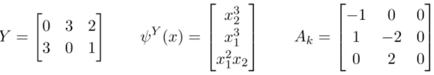
The complex composition matrix Y, the monomial function ψ^Y(x) and the Kirchhoff matrixA_k of the CRN are defined as follows:

Y =

"

0 3 2 3 0 1

#

ψ^Y(x) =





 x³₂ x³₁ x²₁x₂





 A_k=







−1 0 0

1 −2 0

0 2 0







The equations describing the dynamical behaviour of the system can be written in the form of Equation (2.4), that prescribes the kinetic system as in Equation (2.11). The dynamical system and its coefficient matrixM are:

˙

x₁ = 3x³₂−2x³₁

˙

x₂ =−3x³₂+ 2x³₁ M =

"

3 −2 0

−3 2 0

#

By definition it is a kinetic system that is referred to as [M, Y] and the reaction network (Y, A_k) is a dynamically equivalent realization of it. The reaction graph G(Y, A_k) and the reaction graph structure representing the realization (Y, A_k) can be seen in Figures 2.1and 2.2, respectively.

C3

C₂

C₁

1 2

Figure 2.1: The reaction graph G(Y, Ak)

C3

C₂

C₁

Figure 2.2: The reaction graph structure of the CRN (Y, Ak)

(22)

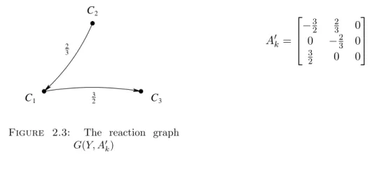
Chapter 2. Basic Notions 14 It will be shown later in Section 5.3.1 that the kinetic system [M, Y] has several dynamically equivalent realizations, one of them is the CRN (Y, A⁰_k). The reaction graphs of the realizations (Y, A_k) and (Y, A⁰_k) are very similar to each other, although these realizations are structurally different. Besides the isomorphism of the graphs the labels of the corresponding edges must be the same as well, and this latter property is not fulfilled by the graphsG(Y, Ak) and G(Y, A⁰_k).

_2 3

_ 3

2 C3

C₂

C₁

Figure 2.3: The reaction graph G(Y, A⁰_k)

A⁰_k =







−³₂ ²₃ 0 0 −²₃ 0

3

2 0 0







2.5.2 Example 2 – Canonical realization of a kinetic system

The following kinetic system was introduced previously as Example 3 in [35].

˙

x1=x1x²₂−2x²₁+x1x²₃

˙

x₂=−x²₁x²₂+x₁x²₃ (2.19)

˙

x₃=x²₁−3x₁x²₃

This polynomial system can be originated from the matrix equation ˙x = M1 ·ϕ(x), where

M1=







1 0 −2 1

0 −1 0 1

0 0 1 −3





 ϕ(x) = h

x₁x²₂ x²₁x²₂ x²₁ x₁x²₃ i>

It can be seen that this polynomial system fulfils the condition of Proposition2.4, therefore it is a kinetic system. But there is no realization on the setC₁={X₁+ 2X₂,2X₁+ 2X₂,2X₁, X₁+ 2X₃} of complexes characterized by the monomial function ϕ. It can be checked for example by trying to find a dense realization using Algorithm 1. There exists at least one realization with a given set of complexes if and only it there is a dense realization on the same set of complexes. From the properties of polynomials it follows that these complexes must be included in the set of complexes of any realization, but in this case other elements are also necessary.

By the application of the method presented in [6] one can obtain a dynamically equivalent realization, and at the same time a suitable set of complexes. During this method every monomial in every dynamical equation of the polynomial system determines a reaction.

For example, in the case of the equation ˙x2 =−x²₁x²₂+x1x²₃ the obtained reactions are:

(23)

−x²₁x²₂: 2X1+ 2X2 1

−→2X1+X2

+x₁x²₃: X₁+ 2X₃ −→¹ X₁+X₂+ 2X₃ The elements of the defined setC₂ of complexes are the following:

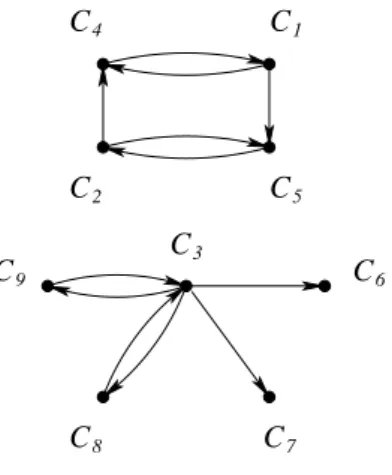
C₁ =X₁+ 2X₂ C₂= 2X₁+ 2X₂ C₃ = 2X₁+X₂ C₄ = 2X₁ C5 =X1 C6= 2X1+X3 C7 =X1+ 2X3 C8 = 2X1+ 2X3

C9 =X1+X2+ 2X3 C10=X1+X3

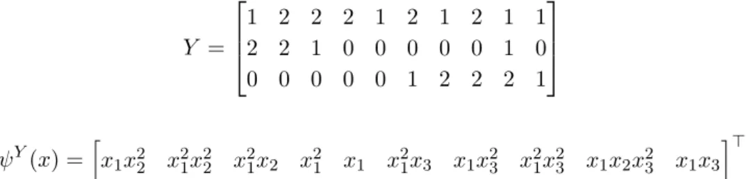
The set C₂ characterizes the complex composition matrixY and the monomial function ψ^Y of the canonical realization:

Y =







1 2 2 2 1 2 1 2 1 1 2 2 1 0 0 0 0 0 1 0 0 0 0 0 0 1 2 2 2 1







ψ^Y(x) = h

x₁x²₂ x²₁x²₂ x²₁x₂ x²₁ x₁ x²₁x₃ x₁x²₃ x²₁x²₃ x₁x₂x²₃ x₁x₃ i>

The computed reactions define the Kirchhoff matrix and the reaction graph as well.

Ak=







−1 0 0 0 0 0 0 0 0 0

1 −1 0 0 0 0 0 0 0 0

0 1 0 0 0 0 0 0 0 0

0 0 0 −3 0 0 0 0 0 0

0 0 0 2 0 0 0 0 0 0

0 0 0 1 0 0 0 0 0 0

0 0 0 0 0 0 −5 0 0 0

0 0 0 0 0 0 1 0 0 0

0 0 0 0 0 0 3 0 0 0







C

C C

C

C C

1 2

3

4

5

6 7

8 9

C₁₀

1 1

1 3

2 1 1

Figure 2.4: The reaction graph of the canonical realization

In order to obtain the form of Equation (2.12) the equation ˙x = M₁ ·ϕ(x) defining the dynamics of the kinetic system needs to be rewritten as ˙x = M₂ ·ψ^Y(x). The additional monomials appear in these equations with zero coefficients, therefore the defined dynamics is unchanged. With these notations the equation M₂·ψ^Y(x) = Y · A_k·ψ^Y(x) holds, that is the special case of Equation (2.12) for dynamically equivalent realizations, where the matrices T⁻¹ and ΨT are identity matrices. The coefficient matrixM₂ is as follows:

(24)

M2 =







1 0 0 −2 0 0 1 0 0 0

0 −1 0 0 0 0 1 0 0 0

0 0 0 1 0 0 −3 0 0 0







2.5.3 Example 3 – Linear conjugacy of kinetic systems

The kinetic system examined in this section was introduced in [24] as Example 2.

˙

x₁ = 1−x₁−x²₁+x₂x₃

˙

x₂ = 2x₁−2x₂x₃−2x²₂+ 2x²₃ (2.20)

˙

x₃ =x₁−x₂x₃+x²₂−x²₃

The linear optimization based method for computing realizations presented in Section 2.4 can be applied only if the set of complexes is fixed. Therefore, the set is fixed to contain only the complexes defined by the monomials, and this kinetic system is denoted as [M, Y], where

M =







1 −1 −1 1 0 0

0 2 0 −2 −2 2

0 1 0 −1 1 −1





 Y =







0 1 2 0 0 0

0 0 0 1 2 0

0 0 0 1 0 2







Despite the fact that the polynomial system (2.20) fulfils the conditions of Proposi- tion 2.4, the computation returns that there is no dynamically equivalent realization of [M, Y]. Indeed, the kinetic property means only that there is a realization with some set of complexes, that is not necessarily the actually considered one. Furthermore, in the case of any kinetic system the canonical realization can be generated and it is a dynamically equivalent realization of the model.

Interestingly, the computation of linearly conjugate realizations returns that there exists such a realization with the given set of complexes.

T =







1

2 0 0

0 1 0 0 0 ¹₂





 ΨT =







1 0 0 0 0 0

0 ¹₂ 0 0 0 0 0 0 ¹₄ 0 0 0 0 0 0 ¹₂ 0 0

0 0 0 0 1 0

0 0 0 0 0 ¹₄







The state transformation is defined by the matrixTand it also characterizes the diagonal matrix Ψ_T. By definition the CRN (Y, A_k) has to fulfil the equationY·A_k=T⁻¹·M·Ψ_T.

(25)

1 4

C₃ C₁

C C₂

C₆ C₅

4

1 1 1 1

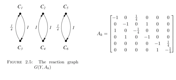
Figure 2.5: The reaction graph G(Y, Ak)

.

Ak=







−1 0 ¹₄ 0 0 0

0 −1 0 1 0 0

1 0 −¹₄ 0 0 0

0 1 0 −1 0 0

0 0 0 0 −1 ¹₄

0 0 0 0 1 −¹₄







In order to have a linear matrix equation in the optimization model, the equation is transformed to the form Y ·A_k ·Ψ⁻¹_T = T⁻¹ ·M and the notation A_b = A_k·Ψ⁻¹_T is applied. For this reason linearly equivalent realizations of a kinetic system [M, Y] with a fixed set of complexes are referred to as the pair (T⁻¹, A_b). In this case the characterizing matrices are

T⁻¹=







2 0 0 0 1 0 0 0 2





 A_b=A_k·Ψ⁻¹_T =







−1 0 ₁₆¹ 0 0 0 0 −¹₂ 0 ¹₂ 0 0

1 0 ⁻¹₁₆ 0 0 0

0 ¹₂ 0 ¹₂ 0 0

0 0 0 0 −1 ₁₆¹

0 0 0 0 1 −₁₆¹







It can be seen thatA_b is also a Kirchhoff matrix and it defines the same set of reactions as the matrix A_k.

(26)

Chapter 3

Dense realizations

There are realizations that have great importance regarding the results presented in this dissertation.

Definition 3.1. A realization of a CRN is called a dense realization if it has the maximum number of reactions.

Dense realizations can be defined in the sets of dynamically equivalent, linearly conjugate or any other kind of realizations of a kinetic system assuming a fixed set of complexes.

The operation of the methods presented in this dissertation depends on a special property of dense realizations. It is drawn up in Proposition 3.3, and was proven in [51].

3.1 Superstructure property

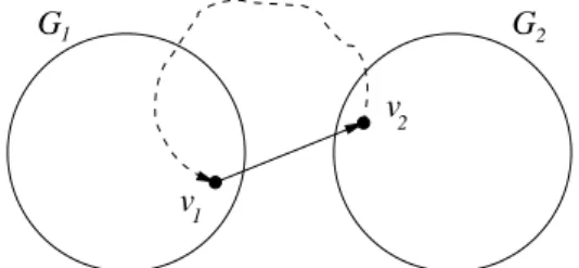
Definition 3.2. LetGbe a set of directed graphs defined on a fixed set of labelled vertices.

A directed graph is called a superstructure considering the set G if it contains every graph in the set as a subgraph and it is minimal under inclusion.

It follows from the definition that for every set G there exists a superstructure and it is unique, as it is the graph whose set of edges is the union of the edges of all graphs inG.

It has been proven in [15] that for any kinetic system the dense linearly conjugate realization defines a superstructure among all linearly conjugate realizations of a kinetic system with a fixed set of complexes. This property holds also for dynamically equivalent realizations. However, during the computations presented in this work a little more is required, and it is proven in Proposition 3.3.

Proposition 3.3. Among all the realizations linearly conjugate to a given kinetic system [M, Y]on a fixed set of complexes and fulfilling a finite set of additional linear constraints the dense realization with the prescribed properties determines a superstructure.

18

(27)

Chapter 3. Dense realizations 19 Proof. In the proof the geometric properties of the set of possible realizations are uti- lized. As it was demonstrated in Section 2.4 the variables of the optimization model defining the linearly conjugate realizations of a kinetic system with a fixed set of complexes are the off-diagonal entries of the matrix A_b ∈R^m×m and the diagonal entries of the matrixT⁻¹ ∈R^n×n. If an ordering is defined on the set of variables the realizations can be represented as points in the Euclidean space R^m²^−m+n. Let the first m²−m coordinates correspond to the off-diagonal entries of matrix A_k ordered column-wise, and the diagonal entries of matrix T⁻¹ be equal to the remaining n coordinates. In this approach the linear constraints of the forms of inequalities and equations are equivalent to halfspaces and hyperplanes, respectively. The set of possible solutions is the intersection of these halfspaces and hyperplanes, consequently it is a convex polyhedron Q ⊆R^m²^−m+n and every point of it corresponds to a realization.

Let us assume that the point D = (d1, . . . , d_m²_−m, . . . , d_m²_−m+n) ∈ Q represents the dense linearly conjugate realization (T⁻¹, A_b) of the kinetic system [M, Y] with the set of prescribed linear constraints.

By the definition of density the point D must have the maximum number of positive values among the coordinates d₁, . . . , d_m²_−m, and since D represents a real linearly conjugate realization, the coordinates d_m2−m+1, . . . , d_m2−m+n are also positive.

Let us assume that the pointR= (r1, . . . , r_m²_−m, . . . , r_m²_−m+n)∈ Qrepresents another linearly conjugate realization that has more positive coordinates thanD. It means that there is an indexi∈ {1, . . . m²−m} for which d_i = 0 andr_i>0 hold.

Since the polyhedron Q is convex, the interval (D, R) is also in Q, and every interior point S of this interval corresponds to a linearly conjugate realization of the kinetic system [M, Y] and fulfils the added constraints as well.

(D, R) ={S ∈R^m

2−m+n |S=c·D+ (1−c)·R, c∈(0,1)} (3.1) From the properties of positive linear combination it follows that all the coordinates that are positive (not zero) inDorR must be positive in the pointSas well. Therefore S has more positive coordinates than D, which is a contradiction.

Consequently, there cannot exist such a pointR∈ Q, and all points in the polyhedronQ can have positive values in only those coordinates where the pointDhas. The realization characterized byDdefines a superstructure among the linearly conjugate realizations of the kinetic system [M, Y] that fulfil the additional linear constraints, and the reaction graphs of these realizations are subgraphs of the reaction graph representingD.

Corollary 3.4. The superstructure property holds for dynamically equivalent realizations considering a set of additional constraints as well. It is because dynamically equivalent realizations are linearly conjugate realizations fulfilling the linear constraints

[T⁻¹]ii= 1 i∈ {1, . . . , n} (3.2) Therefore the set of possible realizations of this model can also be represented as a convex polyhedron and the proof of Proposition 3.3 can be applied.