energies
Article
Energy E ffi ciency in Transportation along with the Belt and Road Countries
Usman Akbar1 , József Popp2 , Hameed Khan3,4 , Muhammad Asif Khan5,* and Judit Oláh2
1 School of Economics and Management, Yanshan University, Qinhuangdao 066004, China;
usman.akbar@outlook.com
2 Department of Management, Faculty of Applied Sciences, WSB University,
41-300 Dabrowa Górnicza, Poland; poppjozsef55@gmail.com (J.P.); juditdrolah@gmail.com (J.O.)
3 School of Economics, Jilin University, Changchun, Jilin 130012, China
4 Department of Economics, Kohat University of Science and Technology, Kohat 26000, Pakistan;
hameed.qec@gmail.com
5 Department of Commerce, Faculty of Management Sciences, University of Kotli, Azad Jammu and Kashmir, Kotli 11100, Pakistan
* Correspondence: khanasif82@uokajk.edu.pk
Received: 29 March 2020; Accepted: 15 May 2020; Published: 20 May 2020 Abstract:China’s huge investment in the “belt and road initiative” (BRI) may have helped improve the economic level of participating countries, but it may also be accompanied by a substantial increase in greenhouse gas (GHG) emissions. The BRI corridors aim to bring regional stability and prosperity. In such efforts, energy efficiency due to increased transport has been overlooked in the recent literature. This paper employed a data envelopment analysis of the slack-based measurement (SBM) for bad output to assess the transport energy efficiency of 19 countries under the BRI economic corridors. By using the most cited transport-related input variables, such as vehicles, labor, motor oil, jet fuel, and natural gas, this study first analyzes the transport energy efficiency by first assuming the output variables individually and then takes two years as a pre- and post-BRI case by considering the aggregated output model. The results show an increase in economic activity but a decline in transport energy efficiency in terms of consumption and emissions.
Keywords: transport energy; data envelopment analysis (DEA); slack-based measurement; economic corridors; belt and road initiative
1. Introduction
The competitive world reflects that transportation energy is an important input for the economy.
Limited access to affordable energy can result in slow and sometimes negative socioeconomic growth in developing countries [1,2]. The population growth, infrastructure development, and trade activities increase the diversity of energy consumption [3–5]. Therefore, energy supply and its consumption are some of the key activities that reflect the economic progress of a country. In the energy sector, the most important topics are energy supplies and revenue generation for the country. In many divisions, energy-intensive transportation has a core function in people’s access to socioeconomic opportunities [6]. If not carefully planned, it will turn the environment into an acid environment and become a greenhouse gas (GHG) producer. This makes GHG emissions from the transport sector one of the serious environmental problems. Therefore, to achieve higher energy efficiency, the negative impact of transport energy should be addressed.
Given the significant impact of transporting energy and the consequent negative impact on the economy, numerous studies have focused on transport efficiency in terms of CO2emissions. Considering
Energies2020,13, 2607; doi:10.3390/en13102607 www.mdpi.com/journal/energies
a recent study, [7] aimed to examine the energy efficiency of Chinese transport-related CO2emissions as one of the variables by using the environmental data envelopment analysis (DEA) approach. Zhou et al. [8] used various operating expenses, including fuel and oil, by using the DEA approach. Their study aimed to benchmark the performance of Chinese third-party logistics in the foreign emerging market. On the other hand, Omrani et al. [9] also considered CO2as a greenhouse gas emitter to assess the energy efficiency of the transportation sector in 20 Iranian provinces. Their findings show that some smaller provinces have higher energy efficiency in the transportation sector than the larger provinces.
Similarly, Du et al. [10] introduce the relationship between the transportation sector and the rest of the Chinese economy as it impacts the generation of carbon dioxide (CO2) emissions. They found that technological advances within the rail sub-sector resulted in a net decrease in CO2emissions. At the same time, the energy-producing industry remains a source of a large amount of CO2emissions.
This study undertakes the five corridors of the belt and road initiative to analyze the efficiencies of 19 countries under its umbrella. China’s “belt and road” initiative (BRI), proposed in September 2013, currently consists of more than 30 countries, including European countries [11]. This rapid economic development with fast urbanization has increased the energy demand in the transport sector, which has a major impact on environmental degradation and social welfare [12]. Recently, with the launch of massive BRI corridors’ investments, energy consumption has increased. Consequently, carbon emissions account for 33.7% due to infrastructure and trade activities, which is up to 61.4% of the global carbon emission each year, including emissions by China [13]. This number is expected to be exceeded due to global transit trade predicted through the BRI corridors. Environment and energy are integrated factors in the undesirable outputs of greenhouse gases (GHG). This makes energy efficiency analysis in transportation very important for policymakers.
This study measures the energy efficiency of transport in 19 countries. Two periods are considered in this research, such as the period before the development of BRI in 2012, and the period after the development of BRI in 2018. By using the DEA model, the input variables consist of energy and non-energy factors as input variables, while desirable and undesirable factors are considered as output variables. These variables do not reflect the bilateral position among the BRI corridor countries.
In other words, we considered the data at the aggregated level. This is due to the fact that BRI respects the global norms, which are facing the challenges of environmental degradation, especially in developing countries, where the global norms are poorly implemented [14]. Therefore, after the major development of the BRI, the domestic and international impacts of the corresponding countries should be considered to evaluate the energy efficiency of the corresponding countries. Each country is treated as a participant with an individual efficiency score, which is considered as an appropriate method in efficiency measurement among the decision-making units (DMUs).
In addition to the actual status of transportation energy efficiency, this study also contributes to the existing literature related to the BRI corridors. It further adds new dimensions to help understand the impact of transportation-related energy emissions in the context of increasing transportation demand due to the corridor developments. Under the implementation of the “belt and road” initiative, there is much literature claiming the regional benefits of the South Asian region, but from 2013 to 2020 (the period of major developments of the six BRI corridors), the literature on the transport energy efficiency of the corridor-related countries is rather scarce. The few latest and closely related works are by Zhao et al. [13], Alam et al. [15], Benintendi et al. [16], and Huang and Li [17]. The quantitative design of this study enables readers to understand the changes in the efficiency of BRI corridor countries after major developments. Along with the “belt and road” studies, there has never been a quantitative data design leading to a specific (international trade and transportation) views of the corridors’ countries.
The remaining paper is organized as follows. In Section2, the literature on transport energy and the existing DEA models has been widely investigated. Section3shows the characteristics of the belt and road initiative, whereas the economic corridors are of particular interest. Section4details the model adopted for analysis, while Section5is related to an illustrative example. Sections6and7discuss the data and variables followed by the results and discussion. Finally, the conclusion summarizes the papers in Section8.
Energies2020,13, 2607 3 of 20
2. Literature
In the immense literature of energy efficiency, scholars have used some adverse factors, such as NOx, SO2, SO3, and CO2 emissions, to estimate the efficiency of transport energy [6,13,18,19].
Increasing the efficiency of the transport sector without considering harmful greenhouse gases may lead to unreliable results. Among all the emission factors mentioned above, the amount of CO2
has the greatest impact on the environment; hence, it can be a better measure of energy efficiency in transportation. According to the U.S. Environmental Protection Agency (www.epa.gov), carbon dioxide emitted through coal, natural gas, and oil accounts for about 81% of global greenhouse gases.
It is evident that CO2is the most suitable factor in GHG that must be considered to obtain effective results. Therefore, the literature review includes two parts. The first is related to the impact of transport energy on efficiency mainly considering CO2emissions and the second part is about the DEA methods used for energy efficiency assessment.
2.1. Impact of Transport Energy
Inevitably, the impacts of transportation energy on the environment, society, and national economy are so great that it has become the focus of many researchers. For instance, Solaymani [20] (2019) studied CO2emission patterns in the transport sector of the seven largest carbon-emitting economies.
He showed that China, the United States, Russia, Canada, India, and Brazil had increased emissions rates between 2000 and 2015, but it is declining in Japan. The author believes that limited private car ownership and an optimized energy structure can reduce carbon emissions [20]. Liu et al. [21] assessed the energy consumption and emissions of China’s transportation by 2050. The results show that by 2050, energy consumption may reach 509-1284 MTCE (Million Tons of Coal Equivalent), which will cause health and economic losses. Talbi [22] analyzes the change in CO2emissions from the Tunisian transport industry and shows the main effects of energy efficiency and fuel rates on reducing CO2
emissions. Zhang et al. [23] estimated the direct energy effect of highway passenger transport in China.
They revealed that with the increase of kilometers, the direct rebound effect in different regions of China would be different. However, the effectiveness of central regions is often better than that of other regions. Similar to Solaymani [20], Lipscy and Schipper [24] also used the Japanese transportation industry as an example to show that compared with developed economies, Japan stands out in terms of the model structure instead of model energy intensity.
The economic impact has a strong positive correlation with carbon intensity, which requires special attention to reduce cost and protect the environment in terms of GHG reductions [25]. The most recent study of Mariyakhan et al. [19] showed vivid evidence. They found that an increase in human-based technology transfer would increase CO2emissions, while a decrease in infrastructure-based technology transfer would reduce emissions. They further established that innovation and infrastructure development with an increased absorptive capacity could help lessen the carbon intensity of China and the US. Li et al. [26] found that the average CO2emissions of suburban commercial centers were 6.94%
and 26.92%, which are higher than those of urban commercial centers. The CO2emissions of wholesale centers were nearly three times less than those of the inner-city commercial centers. On the other hand, Brătucu et al. [27] recommended information campaigns to raise awareness about the importance of energy usage for the sustainable economic development of Romania. Mofleh et al. [28] found that more than 80% of energy consumption is fuel based, and its demand increases over time. They discussed the level of emissions from energy consumption and analyzed its impact patterns in Malaysia. Ji et al. [29]
found that the total emissions of petroleum consumed by transportation (e.g., water, railway, road, and aviation) are almost equal to the net amount of imported petroleum.
2.2. DEA Methods of Energy Efficiency Analysis
Numerous scholars from different disciplines have repeatedly used data envelopment analysis (DEA) as a tool to obtain valid results based on variable inputs and outputs. Wasim et al. [30], in 2019,
find the economic and environmental efficiency of 20 countries by using the DEA model. The authors show that Australia, China, Japan, Saudi Arabia, and Poland are the most energy-efficient based on their consumption, whereas Brazil, France, and Saudi Arabia are the most efficient in reducing CO2
emissions. Smriti and Khan [31] examined the performance of firms in Bangladesh with an effect as a rapid development as a BRI country. Using the non-parametric DEA model, they found the inefficient determinants. Liu et al. [32,33], in their two studies, used the DEA-based parallel slack-based measure method. Their report assessed the overall efficiency of land transportation, including carbon dioxide emissions caused by rail and road.
DEA can also be used to assess energy efficiency, where GHG emissions are found to be an effective measure. Due to the effective popularity of the performance evaluation method, few scholars have developed DEA models with desired and undesired input and output variables by considering transport energy. Song et al. [34] used undesired output factors and an efficiency slack-based measure model to assess China’s transport efficiency. The results indicate that fuel consumption and excessive emissions are positively related. Similarly, Zhou et al. [7] considered undesirable factors as outputs in order to assess the energy efficiency of 30 regions in China for six years. By using the DEA model, the authors point out that, apart from 2008, the performance in east China is better than that in the midwest China.
Liu et al. [35] conducted a systematic study to build the DEA model only with desirable factors. They discussed different combinations of data that helped in obtaining the results without considering the undesirable factors. Jahanshaloo et al. [36] extended the basic approach of the DEA hypothesis to the non-radial DEA model. The idea goes from minimizing input and maximizing output to improve performance by reducing both input and undesired output while increasing desirable output.
In the traditional DEA modal, decision-making units (DMUs) are rated, where the efficient DMUs are equal to one. In other words, the traditional DEA model, designed by Charnes and Cooper [37]
and pursued by Charnes et al. [38], is unable to multirank efficient DMUs. Hence in DEA, different methods have been introduced, such as virtual frontier DEA (VFDEA), super-efficiency, cross-efficiency, and slacked-based measurement (SBM-DEA). Virtual-frontier DEA uses variable return to scale (VRS).
In VFDEA, the reference and evaluated DMUs are different, which creates the possibility to differentiate between the efficient DMUs, but while assessing efficiencies, the reference decision-making units (DMUs) remain unchanged [39]. The application of the virtual frontier has been used repeatedly. For example, Li et al. [40] evaluated the efficiencies of airlines by using the virtual frontier network SBM.
Wanke and Barros [41] took a further step and used the frontier dynamic range adjustment model of DEA (VDRAM-DEA) to calculate the efficiency of Latin American airlines. Again, in 2017, Barros et al. [42] used VDRAM-DEA to evaluate hydroelectric power stations to discriminate the high-efficiency score. Qin et al. [43] used VFDEA to assess the unified energy efficiencies in coastal areas of China.
In the super-efficiency model, DMU can obtain an efficiency score greater than one, and each DMU is restricted to use itself for evaluation. The super-efficiency DEA model, proposed by Andersen and Petersen [44] in 1993, has been widely used in practical applications in the recent literature. In 2001, Zhu [45] showed that, in general, the DEA sensitivity analysis could be performed. There is a case when the data of the target DMU and the rest of the DMUs are allowed to vary unequally. In the worst case, the efficiency of the test DMU will decrease, while in the other DMUs, the efficiency will increase. Xue and Harker [46] found that even when it is not feasible in the super-efficient DEA model, it is still possible to obtain a complete ranking of the entire observation set. The authors explored the feasibility of a super-efficient DEA model for a DMU efficiency ranking. Lovell and Rouse [47] compared the two super-efficiency models to see if they generate the same score as a regular super-efficiency model. They initiated practical solutions for all DMUs using empirical examples.
Li et al. [48] made post-developments in the super-efficiency DEA model to overcome the deficiencies in the earlier models. Cook et al. [49] used the super-efficiency model to the real-world dataset, assuming the variable returns to scale (VRS). They showed that when the model is feasible, it yields super-efficient scores. Sadjadi et al. [18] assessed the performance investigation of gas companies in
Energies2020,13, 2607 5 of 20
Iran, while the efficiencies of China’s banks were conducted by Avkiran [50] and allocated fixed cost as a complement of other cost inputs by Li et al. [51].
Desirable and undesirable factors in DEA were first proposed by Sexton et al. [52] in 1986 and further perused by Sun and Lu [53] in 2005 as re-profiling for increased discrimination in DEA.
However, the model by Sexton et al. had some errors, for example, the weights in their model may not be acceptable for different types of DMUs. Ramon et al. [54] worked on the weight choice profiling in the calculations of DMU scores, which allowed inefficient DMUs to choose appropriate weights to avoid unrealistic scores. Wu et al. [55] determined the multiplier bundle for each DMU for the efficiency score. Then, they used the Nash equilibrium to find the best-performing DMU among the other well-performing DMUs by using the variable return to scale (VRS) proposition. Yu et al. (2010) adopted the same method to design different information-sharing states, which helped in analyzing the supply chain performance. Falagario et al. [56] used good and bad outputs in the DEA-cross efficiency approach in a case study of an Italian public agency for the selection of the best supplier among eligible candidates. All of the bids were assessed equally. Liu et al. (2017) considered undesirable outputs to evaluate the eco-efficiency in coal-fired power plants using the DEA-cross efficiency model [32].
Marbini et al. [57] adopted a similar methodology based on DEA to identify suppliers’ performances in supply chain sourcing issues. Djordjevi´c and Krmac [58] led an assessment under a joint production context by applying the non-radial DEA approach. The approach takes into account energy and non-energy inputs as well as desired and undesired outputs to the transport energy and environmental efficiency (EEE) evaluation.
A slack-based measure (SBM) was found to be another finer measure in DEA with the help of the efficiency score and in the presence of good and bad outputs. After increasing the efficiency score, non-zero input and output slack are likely to occur. In general, these non-zero relaxation values are rather inefficient. Therefore, to fully measure the inefficiency of the DMU, it is important to consider the inefficiency represented by the non-zero slacks in the context-dependent DEA [59]. The original DEA model evaluates each DMU with a set of the most favorable performance indicator weights.
The effective DMU obtained from the DEA construction is an effective frontier. In the most favorable cases, the original DEA can be considered to identify a good (expected output) performance [60].
Chang et al. [61] performed slack-based measurements using DEA to calculate the environmental efficiency concerning the transportation system in China. They found that China lacks the ecological efficiency of the transportation industry; however, there is still room to reduce GHG emissions and energy consumption for a better performance. Hsiao et al. [62] proposed a method based on the fuzzy super-efficiency slack-based measure DEA. They analyzed the operating performance of 24 commercial banks facing loan and investment problems. They found that slack-based measures of efficiency have a higher ability to assess bank efficiency. Bao et al. [63] also used DEA to calculate the ranking of the effective DMU from the linear program output. They compromised the conventional ranking method based on slack. Watto and Mugera [64] estimated the efficiency of groundwater use in cotton production in Punjab, Pakistan. DEA subvectors and relaxation-based models were used to calculate groundwater use efficiency. The results showed that the degree of technical inefficiency is very low, and water purchasers are less efficient than pipeline well owners.
It would be suitable to know a little more about the selected case of “belt and road” economic corridors.
The next section gives a brief background of the selected six economic corridors and their countries.
3. Characteristics of the BRI Corridors
There are several countries in Asia, Europe, Africa, the Middle East, and the Americas. These countries are becoming a part of the BRI global development strategy, aiming to maintain regional prosperity and stability in line with China’s long-term policy. The investment plans, in the BRI, dominantly taking the form of six economic corridors. Countries in the corridors, namely Belarus, Bangladesh, China, Cambodia, Germany, India, Kazakhstan, Kyrgyzstan, Myanmar, Malaysia, Mongolia, Poland, Pakistan, Russia, Thailand, Turkmenistan, Tajikistan, Uzbekistan, and Vietnam, aim to realize
economic integration within bilateral as well as multilateral means. These countries are the main stakeholders in the BRI economic corridors. To date, many investment plans, including infrastructure development, have been completed (www.beltroad-initiative.com). Subsequently, industrial and trade services in these countries have been improved and attracted global investment. Figure1shows the GDP in billions of dollars; we can see the relative contribution of the countries along the BRI economic corridors. Compared with the year 2012, in 2018, after six years of developments, the individual GDP of these countries has undergone major changes, which is evident by their economic progress.
Energies 2020, 13, x FOR PEER REVIEW 7 of 21
industrial and trade services in these countries have been improved and attracted global investment.
Figure 1 shows the GDP in billions of dollars; we can see the relative contribution of the countries along the BRI economic corridors. Compared with the year 2012, in 2018, after six years of developments, the individual GDP of these countries has undergone major changes, which is evident by their economic progress.
Figure 1. GDP of countries under six economic corridors at pre- and post-BRI (Belt and Road initiative) stages. Source: The World Bank.
On the contrary, despite the completion of many road, rail, and waterway infrastructure projects throughout the BRI corridor countries, most of the investments have occurred, especially in areas that have already been developed (see the report, “The Route Controversy”, by Kaiser Bengali). As a result, it affects overcrowding in urban areas. It deprives developments in rural areas, and this imbalance is a root cause of many other factors leading to inefficient transport energy. For some countries, huge investments in transport infrastructure may not be as effective in terms of environmental efficiency as others in other BRI countries. This means that some countries may have economic potential, but there are still forms of energy inefficiency, e.g., the additional energy consumption and emissions, which results in relatively poor contributions to the GDP and social health benefits.
This study aimed to find out the transport energy efficiency of 19 countries and 6 BRI corridors to investigate the transport efficiency after major developments in these countries. Hence, we designed Figure 2, which provides an overview of the number of corridors and countries considered in this study. The six corridors are indicated by different line colors. The countries are represented by the dots irrespective of the size of the countries. Even though two corridors may pass through the two different parts of the country, it is still connected with a single dot for presentable purposes. The new "Eurasian Continental Bridge Economic Corridor" includes China, Kazakhstan, Russia, Belarus, Poland, and Germany. It is obvious from the name of the corridor that the "China-Mongolia-Russia Economic Corridor" includes three countries. The "China-Central Asia-West Asia Economic Corridor" currently includes Kazakhstan, Kyrgyzstan, Tajikistan, Uzbekistan, and Turkmenistan, which coincides with the Eurasian Continental Bridge Corridor. The "China-India Peninsula Economic Corridor" includes China, Myanmar, Thailand, Cambodia, Malaysia, and Vietnam. The
"China-Pakistan Economic Corridor" runs through Pakistan. It has a higher importance than the other corridors because of its strategic location. Finally, there is a "Bangladesh-China-India-Myanmar Economic Corridor". In addition to the country name, the numbers in parentheses represent the total number of inland registered vehicles.
Figure 1.GDP of countries under six economic corridors at pre- and post-BRI (Belt and Road initiative) stages. Source: The World Bank.
On the contrary, despite the completion of many road, rail, and waterway infrastructure projects throughout the BRI corridor countries, most of the investments have occurred, especially in areas that have already been developed (see the report, “The Route Controversy”, by Kaiser Bengali). As a result, it affects overcrowding in urban areas. It deprives developments in rural areas, and this imbalance is a root cause of many other factors leading to inefficient transport energy. For some countries, huge investments in transport infrastructure may not be as effective in terms of environmental efficiency as others in other BRI countries. This means that some countries may have economic potential, but there are still forms of energy inefficiency, e.g., the additional energy consumption and emissions, which results in relatively poor contributions to the GDP and social health benefits.
This study aimed to find out the transport energy efficiency of 19 countries and 6 BRI corridors to investigate the transport efficiency after major developments in these countries. Hence, we designed Figure2, which provides an overview of the number of corridors and countries considered in this study. The six corridors are indicated by different line colors. The countries are represented by the dots irrespective of the size of the countries. Even though two corridors may pass through the two different parts of the country, it is still connected with a single dot for presentable purposes. The new
“Eurasian Continental Bridge Economic Corridor” includes China, Kazakhstan, Russia, Belarus, Poland, and Germany. It is obvious from the name of the corridor that the “China-Mongolia-Russia Economic Corridor” includes three countries. The “China-Central Asia-West Asia Economic Corridor” currently includes Kazakhstan, Kyrgyzstan, Tajikistan, Uzbekistan, and Turkmenistan, which coincides with the Eurasian Continental Bridge Corridor. The “China-India Peninsula Economic Corridor” includes China, Myanmar, Thailand, Cambodia, Malaysia, and Vietnam. The “China-Pakistan Economic Corridor”
runs through Pakistan. It has a higher importance than the other corridors because of its strategic location. Finally, there is a “Bangladesh-China-India-Myanmar Economic Corridor”. In addition to the country name, the numbers in parentheses represent the total number of inland registered vehicles.
EnergiesEnergies 2020, 13, x FOR PEER REVIEW 2020,13, 2607 8 of 21 7 of 20
Figure 2. Belt and road economic corridors with countries and inland vehicles.
4. Model
This paper uses the slack-based measurement of efficiency (SBM) by Cooper et al. [65]. It considers undesirable and desirable outputs relative to less input resources to recognize the transport energy as efficient. First, we take an undesirable output model (SBM-BAD) to analyze the efficient decision-making units (DMUs), and then the additive model is used to identify the DMUs with weak efficiencies, which appears to be efficient in SBM-BAD. The efficiency score is not measured explicitly but is implicitly present in the slacks. Whereas the efficiency score only reflects the Farrell (=weak) efficiency, the ADD-efficient DMU reflects all the inefficiencies in both inputs and outputs.
4.1.A Slack-Based Measure of Efficiency
The basic SBM (slack-based measure), which was introduced by Tone [66], in 2001, has the two properties. Firstly, the measure is unit invariant, and secondly, the measure is monotonously decreasing. Tone has formulated it with the following fractional program:
ρ = ∑ ∑ . (1)
The ratio ( − )/ evaluates the relative reduction rate of input ; therefore, (1⁄ ) ∑ ( − )⁄ corresponds to the mean proportional reduction rate of inputs. Similarly, the second term ( − )/ evaluates the relative proportional expansion rate of output and (1⁄ ) ∑ ( + )⁄ is the mean proportional rate of output expansion. Further, the weights can be assigned to inputs and outputs as follows:
ρ = ∑ /
∑ / , (2)
where:
ρ = Efficiency;
= Input variable of unit ;
= Output variable with ;
= Excesses in inputs; and
= Growth rate.
Figure 2.Belt and road economic corridors with countries and inland vehicles.
4. Model
This paper uses the slack-based measurement of efficiency (SBM) by Cooper et al. [65]. It considers undesirable and desirable outputs relative to less input resources to recognize the transport energy as efficient. First, we take an undesirable output model (SBM-BAD) to analyze the efficient decision- making units (DMUs), and then the additive model is used to identify the DMUs with weak efficiencies, which appears to be efficient in SBM-BAD. The efficiency score is not measured explicitly but is implicitly present in the slacks. Whereas the efficiency score only reflects the Farrell (=weak) efficiency, the ADD-efficient DMU reflects all the inefficiencies in both inputs and outputs.
4.1. A Slack-Based Measure of Efficiency
The basic SBM (slack-based measure), which was introduced by Tone [66], in 2001, has the two properties. Firstly, the measure is unit invariant, and secondly, the measure is monotonously decreasing.
Tone has formulated it with the following fractional program:
ρ= 1 m
Xm i=1
xio−s−i xio
! 1 s
Xs r=1
yro+s+r yro
!−1
. (1)
The ratio
xio−s−i
/xio evaluates the relative reduction rate of input i; therefore, (1/m)Pxio−s−i
/xio corresponds to the mean proportional reduction rate of inputs. Similarly, the second term
yro−s+r
/yro evaluates the relative proportional expansion rate of outputrand (1/s)Pyro+s+r
/yrois the mean proportional rate of output expansion. Further, the weights can be assigned to inputs and outputs as follows:
ρ= 1
− 1
m
Pm
i=1w−is−i/xio
1+1s Psr=1w+r s+r /yro
, (2)
where:
ρ=Efficiency;
xo=Input variable of uniti;
yo=Output variable withr;
s−=Excesses in inputs; and r=Growth rate.
WithPm
i=1w−i =mandPs
r=1w+r =s. This weight selection reflects the importance of the outputr being proportional to its average magnitude. The input weights can be determined analogously.
DEA generally allows more output to be produced with relatively few inputs as an efficiency criterion. A further extension to SBM, including the undesirable outputs, enhances the rationale of the method. Seiford and Zhu [67] proposed the original DEA model in 2002 with desirable (good) and undesirable (bad) output methods. Later, the slacked-based measurement was modified by William Cooper et al. [65], which addressed the environmental inefficiencies by considering the undesirable output, such as greenhouse gas emissions. However, the efficiency scores of DMUs, having an undesirable output, are different under various returns to scale models. One method is to convert the undesirable outputs into desirable outputs, but this may cause the deformation of the efficient frontier and consequently may result in different efficiency scores. Therefore, we used a modified SBM model with an undesirable output.
Suppose that there are n DMUs, each having three factors: input x, desirable output yg, and undesirable outputyb, represented by three vectorsx∈ Rm,yg∈Rs1, andyb∈Rs2, respectively.
We define the matricesX,Yg, andYbas follows:
X=h x1 · · · xn
i∈Rm×n, (3) Yg= [y1g · · · yng] ∈Rn×s1, (4) Yb= [yb1 · · · ybn] ∈Rn×s2. (5) We assumeX>0,Yg>0, andYb>0, and then define the production possibility set as:
P=nx, yg, yb
x≥Xδ,yg≤Ygδ, yb≥ Ybδ,δ≥0o
, (6)
whereδ ∈ Rn is the intensity vector. The above definition corresponds to the constant return to scale technology. According to the definition of the SBM-bad output model, aDMUo
x0, yog,ybo is efficient in the presence of an undesirable output if there is no vector
x, yg, yb
∈ P, such that x0≥x, ygo ≤yg,ybo≥ybwith at least strict inequality. In accordance with this definition, the modified SBM of William Cooper et al. [65] in the case of one input, one good output, and one bad output is as follows:
ρ∗ =min 1− 1
m
Pm i=1
s−i xio
1+s 1
1+s2
Ps1
r=1 srg
ygro +Psr=12 sbr
ybro
. (7)
Subject to:
xo=Xδ+s−, (8)
ybo =Ybδ+sb, (9)
yog=Ygδ−sg, (10)
∴s−, sg, sb, δ ≥0. (11) The function is strictly decreasing concernings−i(∀i),sgr(∀r)andsbr(∀r). The objective value must satisfy the condition 0< ρ∗ ≤ 1. The vectorss− ∈ Rm correspond to excess in inputs andsb ∈ Rs2 corresponds to excess in bad inputs, whilesg ∈ Rs1 represents shortages in good outputs. In the presence of the undesired output, ifDMUohas optimal efficiencyρ∗=1, or when the slacks are equal to zero, i.e.,s−, sg, sb=0, then the decision-making unitDMUois called efficient. If theDMUohas
Energies2020,13, 2607 9 of 20
low efficiency, i.e., ρ∗ <1, then it can be improved by reducing excessive inputs and bad outputs, and hence increasing the good output growth. The function ρ∗is a decreasing function, wheres−i/xio andsbr/ybroare bounded by 1, whereassrg/ygrois unbounded.
Similar to the basic weighted SBM function, the weighted ratio of good to bad output variables can also be imposed on the SBM-bad output method. Therefore, we can apply weights to the objective function as follows:
ρ∗=min 1− 1
m
Pm i=1
w−is−i xio
1+s 1
1+s2
Ps1
r=1 wgrsrg
ygro +Psr=12 wbrsbr
ybro
, (12)
where wi, wrg, and wbr represent the weights to the input i, good outputs r (desirable outputs), and bad outputsr (undesirable outputs), respectively. Additionally, Pm
i=1w−i = m, w−i ≥ 0(∀i), Ps1
r=1wrg+Psr=12 wbr =s1+s2,wgr ≥0(∀r), andwbr ≥0(∀r). 4.2. The Additive Model
By definition,DMUois ADD efficient if and only ifs−∗=0,sb∗=0 andsg∗ =0. However, it should be noted that for real efficiency, the efficiency scoreρ∗is not explicitly measured but implicitly present in the slacks, such ass−∗,sb∗, andsg∗(even whenρ∗ =1). The proof of this theorem can be found in Ahn et al. [68]. Here, however, it is sufficient to define thatxbo =xo−s−∗,bybo =yb0−sb∗, andybgo = y0g+sg∗. Then,
ˆ
xo, ˆybo, ˆygo
is ADD efficient.
5. Illustrative Example
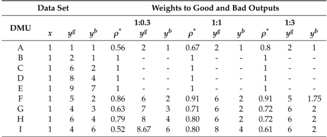
In this section, we will use a model as an example to show a simple slack-based model with a weight selection scheme, which has an undesired output (SBM-bad). William W. Cooper et al. [65] also showed this example in their book. There are nine DMUs with one input and two outputs, e.g., one is a good output, and the other is considered as a bad output.
Firstly, the input factors of all DMUs remain the same. Further, there are three different weights assigned to test the results. It can be seen that as the weights change from good to bad, the projection changes from an increase in good output to a decrease in bad output, as shown in Table1. We also consider that the inputs are the maximum for all DMUs outputs. For this purpose, we consider equal weights for good and bad outputs, e.g., 1:1. With the help of the additive model, we can find out the weak efficiency of the efficient DMU, i.e., DMU “I”. It has an efficiency score equal to one (ρ∗ =1), but it is considered a weak efficiency ass−b =1, see, for example, Table2. It implies that room for trade-offs in terms of input exists in search of better efficiency.
Table 1.Data set with undesirable output and weight effects in the Slack Based Measurement.
Data Set Weights to Good and Bad Outputs
DMU 1:0.3 1:1 1:3
x yg yb ρ* yg yb ρ* yg yb ρ* yg yb
A 1 1 1 0.56 2 1 0.67 2 1 0.8 2 1
B 1 2 1 1 - - 1 - - 1 - -
C 1 6 2 1 - - 1 - - 1 - -
D 1 8 4 1 - - 1 - - 1 - -
E 1 9 7 1 - - 1 - - 1 - -
F 1 5 2 0.86 6 2 0.91 6 2 0.91 5 1.75
G 1 4 3 0.63 7 3 0.71 6 2 0.72 6 2
H 1 6 4 0.79 8 4 0.80 6 2 0.72 6 2
I 1 4 6 0.52 8.67 6 0.80 8 4 0.61 6 2
Table 2.SBM with good and bad outputs and slacks with the additive model.
DMU x yg yb ρ* s− s+g s−b Ref
A 2 1 1 1 0 0 0 A
B 3 2 1 0.67 0 1 0 A
C 2 6 2 0.80 0 0 1 A
D 4 8 4 0.36 1 2 3 A
E 6 9 7 0.23 0 4 6 A
F 5 5 2 0.32 3 3 1 A
G 6 4 3 0.25 3 4 2 A
H 8 6 4 0.18 2 6 3 A
I 2 4 1 1 0 0 1 A
6. Performance Measuring Variables
The transport sector is more challenging when considering developing countries. We analyzed the valuable results of the models by using the most cited variables to compare the transport efficiencies of 19 countries along the “belt and road”. This study considered several infrastructure variables, such as inland vehicles, energy consumption, ton-kilometer (TKM), and passenger-kilometer (PKM) [69,70].
We selected five input variables and four output variables to analyze energy and environmental efficiency. Similar to Li et al. [71], the input factors for evaluating energy efficiency in this study included energy and non-energy variables. The numbers of registered vehicles as resources and the numbers of employed persons as national capital were considered as non-energy variables. On the other hand, the consumption of oil, natural gas, and jet fuel were considered as energy variables, based on the research of Zhu et al. in 2014 [7]. To measure transport efficiency, we used desirable and undesirable output factors. Passenger kilometers (PKM) and ton-kilometers (TKM) were used as good outputs. PKM represents the transport of a passenger in kilometers, while TKM is a measure of freight volume and represents one ton per kilometer of road, rail, and aviation, as adopted by Cui and Li [39].
Additionally, GDP is considered as a desirable output and CO2emission as an undesirable output; see Table3for the list of input and output factors. It is worth mentioning that few scholars have turned bad output (undesired) into good output (desired), see, for example, the same factors used in the recent study by Omrani to assess energy efficiency in Iranian provinces [9].
Table 3.Selected inputs and outputs for transport energy efficiency analysis.
Variables Unit of Measure Source
Non-Energy Inputs
x1 Inland vehicles in numbers CEIC (Census and Economic Information Center)
x2 Labor total employed persons World Bank
Energy Inputs
x3 Vehicle oil Thousand barrels per day Census and Economic Information Center and Organization for Economic Cooperation and
Development x4 Natural gas Thousand barrels per day
x5 Jet fuel Thousand barrels per day Desirable Outputs
y1g GDP International Dollar World Bank
y2g PKM Million passenger kilometers World Bank
y3g TKM million tones kilometers World Bank
Undesirable Output
yb4 CO2emissions million tones Our World in Data
Raw data were collected for 2012 as a year before the start of the “belt and road” initiative. 2018 was considered as the year after the major industrial and transport infrastructure development projects of the “belt and road” initiative took place. The raw data is shown in Table4. In the adopted DEA model, CO2emissions were collected as poor output variables.
Energies2020,13, 2607 11 of 20
Table 4.Raw data for countries of BRI corridors in the year 2012 and 2018.
DMU Inland
Vehicles Labor Vehicle Oil Natural Gas Jet Fuel Gross Domestic Products
Passenger Kilometers
Tons of Kilometers
CO2 Emission
MNG2012 2290 1,056,441 25.0 9.1 0.8 27,547,965,886 2970.40 141.00 26,189,690
MMR2012 3100 463,448,734 34.0 7.0 1.0 211,527,658,640 5163.00 5103.00 10,950,234
KHM2012 3400 7,197,416 40.0 9.1 1.5 41,478,767,114 45.00 6967.00 5,333,522
TKM2012 4700 2,395,746 129.4 25.0 9.0 64,453,951,973 1811.00 1824.77 64,532,904
KGZ2012 4800 514,400 36.0 20.7 1.1 16,073,746,544 75.80 3821.92 9,999,826
TJK2012 6300 2,291,000 12.0 3.5 0.7 18,581,086,820 24.00 114.00 2,906,292
BEL2012 24,500 4,578,483 211.1 25.3 18.0 165,366,731,946 8977.00 138,627.83 63,674,757
BGD2012 43,400 58,072,936 109.8 5.4 6.8 421,488,777,536 8787.00 681,520.31 65,602,526
UZB2012 57,000 13,700,815 63.5 28.0 2.8 173,333,084,074 3437.80 13,984.37 11,5121,942
VNM2012 80,487 51,668,650 368.0 106.4 17.6 436,080,931,087 4558.00 17,455.98 135,375,323
KAZ2012 98,231 8,507,358 3747.4 88.9 6.8 369,196,224,019 18,498.00 3828.76 23,386,0799
PAK2012 157,656 56,010,000 402.3 78.2 15.0 777,020,079,943 20,619.00 619,676.80 159,727,596
POL2012 329,799 15,590,675 571.0 87.6 11.6 883,754,778,000 15,724.00 458,576.41 324,216,621
MYS2012 627,753 12,541,200 757.4 191.7 52.1 658,983,690,152 2321.36 240,360.21 215,895,218
THA2012 1,423,580 38,950,101 1250.0 132.4 87.5 980,230,501,537 8032.00 6026.17 293,664,431
RUS2012 3,141,551 71,541,667 3119.3 789.4 269.5 3,603,976,213,817 139,842.00 2,594,549.63 1,726,099,500
DEU2012 3,394,002 42,006,000 2351.6 426.8 187.0 3,429,348,441,084 80,210.00 314,445.67 815,197,409
IND2012 3,595,508 463,448,734 5155.7 363.0 115.0 6,097,525,693,324 1,046,522.00 2,430,714.25 1,983,758,813 CHN2012 19,306,435 767,040,000 10,242.3 2157.9 462.3 15,013,124,413,267 795,639.00 6,663,629.02 9,633,899,303
BGD2018 453,850 69,706,733 175.7 10.0 8.0 625,926,138,171 10,040.00 681,696.00 88,057,461
BEL2018 419,029 4,975,430 136.2 27.0 4.0 168,288,411,616 6215.00 138,764.00 61,371,793
MNG2018 42,450 1,333,084 28.0 10.0 1.0 38,819,139,033 973.00 169.00 30,390,657
KHM2018 53,224 9,230,114 28.0 13.0 3.0 62,878,417,548 45.00 6995.00 7,938,275
KGZ2018 65,810 2,654,625 40.0 16.0 0.5 21,770,524,329 43.00 3861.92 10,433,128
MMR2018 72,152 24,744,320 25.0 13.0 2.2 318,062,369,686 4163.00 5128.00 25,333,224
TKM2018 72,795 2,675,573 515.2 35.0 10.0 100,220,117,332 2340.00 2340.00 72,702,485
TJK2018 79,870 2,560,157 16.0 4.0 0.4 27,858,305,681 28.00 130.00 5,711,373
UZB2018 823,300 15,555,364 52.6 20.0 2.0 250,196,959,373 4294.00 14,037.00 98,998,947
KAZ2018 1,157,121 9,262,539 248.0 101.0 6.8 452,130,663,560 19,241.00 4076.76 292,588,517
VNM2018 2,143,404 57,249,411 522.0 146.0 34.0 631,390,326,246 3542.00 17,978.00 198,826,549
PAK2018 2,695,795 75,143,667 498.2 176.0 17.0 1,048,295,564,439 24,903.00 620,175.00 198,809,969
POL2018 6,196,359 18,176,456 684.6 106.0 21.7 1,093,233,066,641 9466.00 459,261.00 326,604,543
MYS2018 8,795,736 15,788,572 813.8 300.0 69.0 889,139,386,019 2029.00 241,174.00 254,575,871
THA2018 13,062,265 38,917,441 1477.8 188.0 116.0 1,173,668,257,359 8032.00 7504.00 330,839,584
RUS2018 33,613,762 72,736,316 3228.4 819.0 228.0 3,763,167,030,947 129,371.00 2,597,778.00 1,692,794,839 IND2018 45,146,945 519,469,299 5155.7 593.0 161.0 9,317,083,079,866 1,149,835.00 2,435,870.00 2,466,765,373
DEU2018 53,957,478 43,228,550 2321.3 490.9 221.0 3,809,392,176,976 79,456.00 316,767.00 799,373,211
CHN2018 281,565,485 783,194,000 13,521.0 3433.9 830.0 22,536,847,278,112 681,203.00 6,677,150.00 9,838,754,028
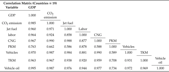
The correlation matrix shows the positive relationships among variables, as shown in Table5.
Table 5.Correlation matrix of the input and output variables.
Correlation Matrix (Countries=19) Variable GDP
GDP 1.000 CO2
emission
CO2emission 0.985 1.000 Jet fuel
Jet fuel 0.960 0.971 1.000 Labor
labor 0.964 0.924 0.858 1.000 CNG
CNG 0.967 0.990 0.988 0.877 1.000 PKM
PKM 0.763 0.662 0.586 0.878 0.588 1.000 Vehicles
Vehicles 0.970 0.987 0.984 0.881 0.990 0.589 1.000 TKM
TKM 0.963 0.967 0.938 0.920 0.959 0.708 0.931 1.000 Vehicle
oil
Vehicle oil 0.995 0.987 0.976 0.944 0.977 0.734 0.972 0.969 1.000
7. Results and Discussions
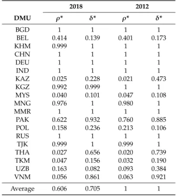
In this section, energy efficiency analysis was performed for 19 countries under the “belt and road” economic corridor. In DEA, generally, the optimal efficiency rating is considered 1, and the closer the value is to 0, the more inefficient it is. The definition of output becomes complicated as the poor output (undesired output) comes in the form of carbon dioxide emissions, and hence, it then links the economic factors, such as GDP, to corresponding efficiencies. Vehicle mileage is associated with service efficiency (ton-kilometers (TKM) in our case). Efficiency is related to passenger- kilometers (PKM), used as ridership in the literature (see, for example, the study of Fielding in 1989 [72]). Variables, such as inland vehicles, energy consumption, tons of kilometer (TKM), and passenger kilometer (PKM), are also considered as some infrastructure variables [69]. In this article, we estimated the proposed DEA model five times. In the first four analyses, we obtained efficiency results with a single output for the year of 2018. This was to observe the specific impact of the transport energy efficiency. First, GDP was taken as an output; the second, third, and fourth model used PKM, TKM, and CO2emissions as outputs. The fifth is the multi-output model, which used the years 2012 and 2018 and used aggregated outputs to comprehensively consider the performance of countries in the economic corridors before and after the belt and road initiative. The five inputs, namely inland vehicles, labor, oil, natural gas, and jet fuel were selected for the evaluation of land, rail, and air transport energy. The production possibility set in our case can be written as:
P=nx1,x2, x3,x4, y1g,yg2, y3g, yb4
x1x2x3x4≥Xδ,yg1yg2y3g≤Ygδ, yb4≥ Ybδ,δ≥0o
. (13)
7.1. Efficiency Analysis with Individual Outputs
The analyses were performed separately with the selected outputs, and the estimated results are shown together in Table6. The rating column in the table shows the efficiency score of the DMUs, where 1 reflects the optimal efficiency. The rank column shows the position of the DMU in comparison with the rest of the selected DMUs. It is notable that fully efficient DMUs with an efficiency score equal to 1 tends to change the efficiency rating when analyzed with different output variables. China (CHN) turns out to be optimally efficient (rating=1) by considering its GDP and TKM. However, it shows a poor performance with PKM (rating=0.64) and CO2(0.24) emissions. On the other hand, India (IND) seems to be very effective when using PKM (rating=1), but it has a poor efficiency with CO2
emissions (rating=0.26). However, Tajikistan (TJK) appears efficient in CO2emissions (rating=1) along with good efficiency scores with the rest of the output variables. One of the reasons could be the
Energies2020,13, 2607 13 of 20
limited use of inland vehicles. On the contrary, Malaysia (MYS), Belarus (BEL), Kazakhstan (KAZ), and Thailand (THA) show poor performance scores in all individual output analyses, while other DMUs remain inconsistent.
Table 6.Efficiency rating and ranks with individual outputs for the year 2018.
DMU With GDP With PKM With TKM With CO2
Rating Rank Rating Rank Rating Rank Rating Rank
BGD 0.279 10 0.076 11 0.709 5 0.410 9
BEL 0.091 19 0.056 13 0.234 10 0.426 8
KHM 0.277 11 0.004 19 0.127 13 1.000 3
CHN 1.000 1 0.644 5 1.000 1 0.243 19
DEU 0.414 7 0.171 8 0.140 12 0.284 16
IND 0.693 6 1.000 1 0.639 7 0.266 18
KAZ 0.139 16 0.099 9 0.005 18 0.367 10
KGZ 0.997 4 0.910 4 0.995 2 1.000 4
MYS 0.158 15 0.007 18 0.146 11 0.315 14
MNG 0.998 3 0.994 2 0.862 4 1.000 2
MMR 0.706 5 0.208 7 0.064 15 0.605 5
PAK 0.195 13 0.074 12 0.353 8 0.327 13
POL 0.209 12 0.033 15 0.284 9 0.329 11
RUS 0.382 8 0.240 6 0.688 6 0.279 17
TJK 1.000 2 0.983 3 0.984 3 1.000 1
THA 0.169 14 0.021 16 0.004 19 0.303 15
TKM 0.103 18 0.039 14 0.009 17 0.430 7
UZB 0.304 9 0.090 10 0.069 14 0.468 6
VNM 0.116 17 0.011 17 0.012 16 0.327 12
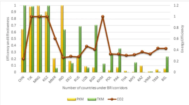
As can be seen in Table6, Tajikistan (TJK=1), Mongolia (MNG=2), and Kyrgyzstan (KGZ=4) are the most efficient borders for carbon dioxide emissions, and they appear to be landlocked countries (Cambodia (KHM) is an exception). Landlocked countries have been deprived of the right of major trade through the straits, so their TKMs rely only on roads, trains, and planes. However, surprisingly, these countries also retain efficiency in PKM, TKM, and GDP. On the other hand, industrially developed countries, such as China (CHN) and India (IND), seem to be effective when using PKM and TKM, but they are not efficient in terms of transport energy emissions (CO2).
It is also evident from Table6that the GDP-efficient countries, such as Tajikistan (TJK=1) and Mongolia (MNG=0.99), excluding China (CHN=1) and Myanmar (MMR=0.70), tend to have less efficiency when analyzed with other output factors, i.e., PKM, TKM, and CO2. The analysis with output variables PKM and TKM was also considered as effective and efficient in terms of the transport energy utilization output (see, for example, Karlaftis [73]). Looking broadly, if we compare the efficiency of PKM, TKM, and CO2emissions, then except the two countries, i.e., Uzbekistan (UZB) and Cambodia (KHM), other countries with an increase in PKM and TKM tend to increase CO2emissions, as shown in Figure3. The increase in personal registered vehicles appears to be one of the causes.
7.2. Efficiency Analysis with Aggregated Outputs
Efficiency is usually measured by the ratio of the weighted sum of the output to the sum of the input factors. The weight of the input factor represents the binding force on the output factor and may become a constraint in the process of improving efficiency, so all input factors have the same weight.
However, the weights to the good and bad output could result in better output, as demonstrated in an illustrative example earlier. Generally, the estimated efficiency specifies the overall efficiency of the input factors considered. The best balance between inputs can improve the efficiency. However, the SMB model is not limited to the input factors but also takes into account the slackness of the output factors to obtain a clearer picture. In this analysis, the weight ratio of good output to bad output is 1:0.5.