AND BONDING WAVE MECHANICS CHAPTER EIGHTEEN

WAVE

MECHANICS AND BONDING

18-1 Introduction

G. N . Lewis, perhaps the dean of American physical chemists, suggested in 1916 that the chemical bond between two atoms consists of a jointly held or shared pair of electrons. To this day, the concept of the shared electron pair bond has much qualitative utility for the chemist. We write, for example

H H . H

H:H, H:C1, H : C : H , -.CrrC'. , H:C:::C:H H H H

to show single, double, and triple bonds. By including nonparticipating electrons, the satisfying octet rule emerged for light-element molecules. Thus

:C1:Ç1:, : p: : 0 . \ H:C1:Ô: , : b : : C: : 0 ;

In each case every atom "sees" an octet of electrons if the shared ones are included.

In addition, the formal charge on each atom is obtained by again counting elec­

trons, but now allowing only half of the shared ones, and noting the excess or deficiency over the net charge of the nucleus plus inner electrons. The formal charges are zero in the preceding examples, except for HCIO, in which CI has the formal charge + 1 and 0 , - 1 . Thus an indication of bond polarity emerges as well.

The electron pair bond and the octet rule give chemically useful pictures of molecular bonding; they are the basis for our writing a bond as a line between atoms. The difficulty in explaining why ordinary Oa is paramagnetic or why N O should have so little tendency to dimerize has been explained quite nicely by Linnett (1964) in a modern extension of the octet rule.

Contemporary wave mechanical treatments support much of these qualitative ideas but, of course, go far beyond them in giving detailed electron density maps, in accounting for bonding with an odd number of electrons, in explaining delocalized pi bonding as in benzene, and in giving molecular energies and other properties.

In this chapter we give a brief account of some of the mathematical methods used and typical results for simple molecules. As may be imagined, the subject is a formidable one both in complexity and in the welter of detailed calculational

759

algorithms that have been developed. Of necessity, therefore, we present here no more than an introduction to a large field of chemical physics.

The mathematical problem of dealing with the simplest common molecule, H2, or more generally, with an AB-type molecule where the atoms are hydrogen-like, can be appreciated by looking at the complete Hamiltonian:

h2 h2 h2

; ( V + V2*) -

5-3—

8TT2^W V 17 ^87T1 2^mA2 ^S7T2^mB

_ + ZB_ + ΖΛ + _ ΖΛΖΒ _ J _ \ ) ( 1 8 1

X ,A, 1 rB,l ΓΑ,2 rB,2 r AB r\2'

where 1 and 2 denote the two electrons, and A and Β the two nuclei. Also, rAB is the internuclear distance; rA i l, that between electron 1 and nucleus A, etc.; and r12 is the interelectronic distance. In practice a major simplification is made at once by dropping the V2 terms for the two nuclei,

H = - 8 ^ [ V ) +2 V 2 ( 2 )( 1] - i h + 7^+7^ + r-) e

δ 7Γ m XrA,l *B,1 rA,2 rB,2/

+ ββίψΒ + ± \ ( 1 8_ 2 )

V 'AB r12'

This approximation, known as the Born-Oppenheimer approximation, can be justified mathematically. A qualitative explanation is that the nuclear masses are so large compared to the electron mass that the electrons adjust instantaneously to the nuclear motions. As a consequence we treat the energy of nuclear motions separately as vibrational energy (as in Section 16-6) and assume that the amount of vibrational energy present simply adds to that of the electronic state. The wave equation, ϋφ = Εφ, is then to be solved for various rAB values, the equilibrium one being that giving the lowest energy (most negative potential energy). Explicit solutions are not possible—only more or less accurate approximations. The big difficulty is in the r12 term which prevents the wave equation from being separated into two one-electron equations.

Two types of mathematical attack have emerged. Both make use of the variation method (Section 16-11), but differ in the manner of choosing the approximation wave function φ. To review the variation method in the present context, if two wave functions, φ± and φ2, are alternative extreme possibilities, the approximation of writing φ = αφχ + άφ2 is used. Equation (16-97) becomes

ρ ^_ f (αΨι + 1>Φύ*Κ(<*ΐΊ + άφ2) dr

ί {αφι + 1>Φύ*(αφι + &φ2) dr ^Αβο' or, on using the definitions of Eq. (16-100), that is,

H ll = j φ1^Ηφ1 dr, H12 = j φλ*Ηφ2 dr,

S

u=j Ψι*Ψι

>

i* = J ^1*^2 dr,

we obtain

(18-4)

a*Hxl + 2abH12 + b2H22

a2S±1 + 2abS12 + b2S22 ' ; U Ô O

(The distinction between H12 and H21 is not necessary here.) The next step is to

obtain the minimum possible Ε for the given choice of φχ and ψ2 as basis functions;

this is done by setting (dE\dd)b = 0 and {dEjdb)a = 0. On carrying out the first differentiation, we obtain

(dE\ = 2aH11 + 2bH12 _ 2aS11 + 2bS12

\ da )b fl»Su + 2abS12 + b2S22 * a2Slx + 2abS12 + b2S22 2a(H11 - ES^) + 2b(H12 - ES12)

a2SllL + 2abS12 + b2S22 or, on setting the derivative equal to zero,

α(Ηιτ - ES^) + b(H12 - ES12) = 0. (18-6) Similarly, on setting the derivative (dEldb)a = 0, we obtain

a(H21 - ES21) + b(H22 - ES22) = 0. (18-7) As simultaneous equations in a and b, the solution is given by the determinant

= 0. (18-8)

C#n —

An equation such as Eq. (18-8) is called a secular equation. Its solution and the evaluation of the various integrals is central to the variation method.

In the valence bond method, approximate wave functions are constructed from those of the separated atoms, complete with electrons. This approach is, in a sense, the quantum mechanical outgrowth of the electron pair bond concept, hence the name. In the second approach, the molecular orbital method, the approximate wave function is constructed from the orbital functions of the atoms (which may be more than just two), to obtain molecular orbital functions. The requisite number of electrons are then assigned into these molecular orbitals.

We take up the valence bond approach in the next section, with emphasis on the Η 2 molecule. The succeeding sections deal with the molecular orbital method, first in terms of H2+, for which exact solutions are possible, and then for H2 and other diatomic molecules. Sections 18-6 and 18-7 carry aspects of the molecular orbital method to triatomic and then polyatomic molecules.

18-2 The Valence Bond Method for the Hydrogen Molecule

The Hamiltonian for the hydrogen molecule is given by Eq. (18-2), after making the usual Born-Oppenheimer approximation. As noted, the equation is not separ­

able because of the e2/r12 term, so no exact solution is possible. The valence bond method was developed by W. Heitler and F. London around 1927 as an approach to the hydrogen molecule problem.

A. Application of the Variation Method

The approximate wave function for the variation method is set up as follows. If atoms A and Β are separated, two possible wave functions are

Φι = 0A(WB(2), Φ2 = 0A(2>AB(1).

That is, electron 1 may stay with atom A and electron 2 with atom B, or vice versa.

The approximate wave function is taken to be a linear combination of the two possibilities, that is,

φ=αφχ + οφ2. (18-9)

The approximate wave function in the valence bond method is thus assembled as a linear combination of the products of the wave functions for the separated atoms.

In the case of H2, atoms A and Β are the same, and H12 = H21 and S12 = S2 1. The integral S1± may be written SX1 = J J ^a*(1)^B*(2)^A(1)^B(2) drx dr2 = ί ^A*(1)^A(1) drx J φΒ*(2)φΒ(2) dr2 = l. Each integral is just the normalization integral S, which is unity. Similarly, S22 = 1. Expansion of the secular equation, Eq. (18-8), therefore gives

π ( # ι ι ± # 1 2 ) Τ ( # n ± H12)S12 R 1 Λ. n

E =

r=sf

or

and

E l = Hl

î+s£

"

E2 = H" - Hi \ (18-12 )

1 — O i 2

If thes e solution s ar e substitute d bac k int o Eqs . (18-6 ) an d (18-7) , t o find th e co - efficients a an d b9 on e obtain s

φ1 = φ1 + φ2 (18-13)

and

Φ2 = ΦΙ-Φ* (18-14) (except for a normalization factor). This result (that a = ± 6 ) is to be expected for

two like atoms; for an A —Β molecule, the coefficients a and b would not be equal.

40 h

F I G . 1 8 - 1 . Plots of the total energy. Coulomb energy, and exchange energy for H2 as a function of internuclear distance. The energy scale is actually Ej{\ + S2). (From C. A. Coulson, " Valence,"

2nd ed. Oxford Univ. Press, London and New York, 1961.)

Integrals of the type Hu are known as Coulomb integrals (two-center in this case since H involves both atoms); those of the type H12 are called exchange or resonance integrals; and those of type S12 are called overlap integrals.

These three types of integrals have been evaluated rather accurately for pairs of hydrogen-like atoms using modern computer methods. Calculations for the case of two hydrogen atoms give the results shown in Fig. 18-1, for example.

The integrals Hn and H12 are negative for most interatomic distances, the latter more so; the sum goes through a minimum around Ι.Ία0, where a0 is the radius of the first Bohr orbit. The integral .S12 may be written .S2, where S is the one- electron overlap integral,

In the actual evaluation of S (and of the /Ts), one uses the elliptical coordinate system shown in Fig. 18-2. The angle φ is that between the xz plane and the plane defined by A, B, and the electron. The calculation of S is relatively straight­

forward and has been made for hydrogen-like wave functions for a variety of η and / values [see Mulliken et al. (1949)]. Some representative results are shown in Fig. 18-3 for the case of two carbon atoms (using the appropriate Zeu). There is not a great deal of difference in S for the various types of orbitals beyond about

1.5 Â (the C—C bond length is 1.54 Â ) , although that for the two pi-bonding type orbitals is distinctly lower than the rest. The 2s-2pa and 2ρσ-2ρσ integrals go through a maximum, and the latter can actually be negative because at small distances oppositely signed lobes of the ρ orbitals begin to overlap (these are pz orbitals if ζ denotes the bond axis, that is, they are ρ orbitals of sigma bonding symmetry).

We can now see that in terms of Eq. (18-11) it is the Coulomb and exchange integrals that make Ελ negative (corresponding to bonding in our sign convention) and that while the overlap integral acts to diminish the denominator (S12 always being less than unity), it does not determine the sign of E±. However, as discussed in Section 17-7, one often uses the rule of thumb that a proper overlap of bonding orbitals is needed for a strong bond to form. The rule is a good one in spite of the preceding comment, since the Coulomb and exchange integrals are often roughly proportional to the overlap integral.

This qualitative use of the overlap idea was extended by L. Pauling to the case of hybrid orbitals. The maximum value of the trigonometric portion gives a measure of the "reach" of an orbital in the direction of its greatest amplitude.

S = j ΦΑ(Ό ΦΒ(Ό dr= j φΑ(2) φΰ(2) dr. (18-15)

y

F I G . 1 8 - 2 . The elliptical coordinate system.

Internuclear distance, A ο

F I G . 1 8 - 3 . Overlap integrals S for various pairs of orbitals. [See R. S. Mulliken, C. A. Rieke, D. Orloff, and H. Orloff, J. Chem. Phys. 1 7 , 1248 (1949).]

The more precise observation is that for a given bond distance, S for sp3, sp2, and sp hybrid orbitals increases in that order.

The second solution, E2, is given by Eq. (18-12) and involves the difference (HX1 — H12). This difference is positive at all internuclear distances, so <f>2 corre­

sponds to a repulsion between the atoms. We speak of φ1 as a bonding wave function and φ2 as an antibonding wave function. The result is characteristic: F o r every com­

bination of atomic wave functions that leads to bonding there is always a related antibonding combination.

The numerical results for the bonding case are that the minimum energy occurs at 0.80 Â and —74 kcal m o l e- 1, as compared with the experimental values (dashed curve in Fig. 18-1) of 0.74 Â and —108.9 kcal m o l e- 1. Note that it is the exchange integral H12 that supplies over 9 0 % of the bond energy. The physical explanation of this integral is that the electrons, being indistinguishable, are n o t localized about the nuclei with which they were associated in the separated atoms, but expand over the system of both atoms. Without this exchange effect only a rather weak bond (given by the H1X contribution) would be expected.

β. The Spin Function

The preceding wave functions are incomplete; they should include the spin func­

tion (Section 16-9C). Recalling the combinations of Eq. (16-92), we have for the possible complete wave functions

[<AAO) ΦΒ(2) + φΑ(2) 0B(1)][«(1) j8(2) - «(2) j8(l)] singlet, (18-16) («(1)«(2)

[0A(1) ΨΒ(2) - φΑ(2) φΒ(1)] β(1) j8(2) triplet. (18-17) («(l)j8(2) + a(2)j8(l)

The restriction of choice to these combinations follows from an alternative state- merit of the Pauli exclusion principle: Every allowable wave function for a system of two or more electrons must be antisymmetric for the simultaneous interchange of the position and spin coordinates of any pair of electrons. This statement implies the usual one that no two electrons can have the same four quantum numbers. The first function of Eqs. (18-17) is symmetric in the spatial wave func­

tions, and so must be antisymmetric in the spin function; as only one possible spin function of this type is available, there is only one complete wave function, and the state is called a singlet state. The triplet state is so called because it is triply degenerate in the spin function; since the wave function is antisymmetric, any one of the three possible symmetric spin functions may be used.

It is customary to designate the spin multiplicity or degeneracy by a left super­

script to the symbol describing the state. Thus the singlet and triplet states of H2 are designated 1Σ% and , respectively. The symbol Σ is used to mean that the angular momentum of the state is zero about the internuclear axis, and g and u inform us that the wave functions are symmetric and antisymmetric with respect to inversion, respectively. The triplet state is a high-energy, repulsive one (Section 19-2A), while the singlet state is the bonding and lowest-energy or ground state of H2. There are, of course, many yet more energetic states than the ζΣη one; these can be regarded as involving the mixing of 2s, 2p, ... orbitals (see Section 19-2).

C. Inclusion of Other Configurations

Somewhat improved results can be obtained for H2 if φ is taken to be

Φ = ΦΑ(\) ΦΒ(2) + φΑ(2) φΒ(1) + α[φΑ(1) ψΑ(2) + φΒ(1) φΒ(2)]. (18-18) The last two terms correspond to H ~ H+ and H+H~, respectively. The variation method is used to find the optimum value for a, and the best calculated value for Ex is now —94 kcal m o l e- 1.

The inclusion of such ionic configurations is often needed in the valence bond method. A molecule is sometimes said to resonate among various structures, the so-called resonance structures. It must be remembered, however, that a single wave function describes the state of the molecule. The so-called resonance struc­

tures are merely the components of a linear combination of wave functions that has been assembled in an effort to approximate the correct one. It is particularly important not to be misled into supposing that the molecule is somehow flickering between different electronic configurations.

18-3 Molecular Orbitals.

The Hydrogen Molecule Ion, H

The hydrogen molecule ion, H2+, is a weakly bound species, and is not one of great chemical importance. It is of interest to us here, however, for two reasons.

First, it is the one molecule for which exact solutions have been obtained. Second, and very important, these solutions give us a set of molecular, one-electron orbitals which are widely used in the approximate description of diatomic molecules generally.

A. Solutions to the Wave Equation

The wave equation for the hydrogen molecule ion is

( _ V « - l - l + -2-U = £fc (18-19) X r^A *B r^AB'

where energy is in rydberg units (1 rydberg = | a.u.—Section 16-2), and rA , rB , and rAB are as defined in Fig. 18-2. Notice that, of course, the difficult r12 term of Eq. (18-2) is absent (and that the usual Born-Oppenheimer approximation is made).

This problem has been solved exactly (not explicitly, but by series expansions) for any value of rAB , which for simplicity we will now denote just as R. It turns out that if the elliptical coordinate system of Fig. 18-2 is used, then the wave equation can be separated into three, or one for each coordinate—much as was done for the hydrogen atom when polar coordinates were used (Section 16-7A).

In the elliptical system, the three coordinates are λ = ( rA + rB)/R, μ = ^Α — rB)jR, and </>, the angle between the xz plane and the plane defined by the nuclei A and B, and the electron. The ζ coordinate is taken to be along the line between the nuclei with the origin at the midpoint. On writing out the Laplacian, V2, for this co­

ordinate system (see Problem 18-8), and expressing φ as

φ = Ε(λ)Μ(μ)Φ(φ), (18-20) the wave equation separates into one in λ only, one in μ only, and another in φ

only. The solution for the φ equation is just

Φ = ém<1>9 (18-21)

where, for physically acceptable solutions, m is restricted to the values 0, ± 1 , ± 2 , e t c For m > 0, one takes linear combinations so as to obtain cos|m|0 and sin|m|0 functions. The procedure is like that for the Φ solutions for the hydrogen atom (Section 16-7B).

In the case of H2+, the m quantum number plays somewhat the same geometric role as does the / quantum number for the hydrogen atom. Consistent with this analogy, the custom is to refer to states of m = 0 as σ states, to those with m = ± 1 as ττ states, and to those with m = ± 2 as δ states. Further, φ can be either symmetric (sign unchanged) or antisymmetric (sign changed) on inversion of a general point through the center of symmetry. We indicate these two situations by the symbols g (gerade in German) and u (ungerade), respectively. We thus have solutions designa­

ted as ag, au, 7Tg, 7Tu , etc. The quantum number associated with the L and M functions is not generally of interest.

The functions φ(ΙσΒ) and φ(1 au) are plotted in Fig. 18-4 as the profile along the H - H axis, the number 1 merely denoting the lowest energy solution. Figurel8-4(a) is for R = 8a0 (a0 is the Bohr radius—Section 16-2), at which separation the elec­

tron density is nearly that for two separate atoms. Each section of each curve is approximately that of the R(r) function for η = 1, ί — 0 of Fig. 16-8. In the case of Φ(1σ8), the sign of the R(r )-like function is the same for both atoms, while in that of φ(1 σα), it is positive for one and negative for the other. Figure 18-4(b) is for R = 2a0 , or for about the equilibrium separation (see below). The Φ(ΙσΒ) function now shows considerable electron density at the midpoint between the two nuclei, corresponding to the Lewis-type formulation Η · H. Finally, in Fig. 18-4(c), the two

F I G . 1 8 - 4 . Normalized wave functions for lae (left) and 1σα (right) ofH2+ along the H - H axis.

(After J. C. Slater, "Quantum Theory of Molecules and Solids," Vol. 1. McGraw-Hill, New York, 1963.)

nuclei are merged (R = 0), and the φ functions are just those for He + . Φ(1σΒ) has become 0(ls) for He + , and φ(1ση) has become φ(2ρ).

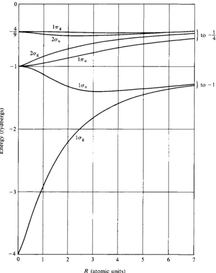
The potential energy for several of these molecular orbitals is shown as a function of R in Fig. 18-5. Internuclear repulsion (the e2\R term) is not included, and the lines terminate at the energy levels for H e+ and for separated Η atoms at the left and right extremes, respectively. Again, the numbers 1 or 2 preceding the symmetry designations are just ordering numbers. The actual energy variation with R, that is,

- 3

- 4 It I I I I I I I

0 1 2 3 4 5 6 7 R (atomic units)

FIG. 1 8 - 5 . Energy levels of H2+ as a function of internuclear separation, omitting the inter­

nuclear repulsion term. (After J. C. Slater, "Quantum Theory of Molecules and Solids," Vol. 1.

McGraw-Hill, New York, 1963.)

including the e2/R term, is shown in Fig. 18-6. We now see that ψ(\σΕ) has an energy minimum at about R = 2a0 or, more exactly, at 1.06 Â. This is the equilibrium bond distance for H2+. The energy at the minimum is —1.2 rydbergs or at —0.2 rydbergs or —(0.2)(13.61) = —2.72 eV relative to the separated H+ + H. This is the H2+ bond energy.

β. Molecular Orbitals

It was noted at the beginning of this section that the solutions for H2+ provide a set of molecular orbitals useful in the description of diatomic molecules, and, in­

deed, of any A—Β bond. It is therefore worthwhile to take a further look at these functions. Because of the minimum in its energy (Fig. 18-6), ψ(ΙσΒ) is called a

0 | 1 1 1 1

0 2 4 6 8 10 12 14 R (atomic units)

F I G . 1 8 - 6 . Energy levels o/H2+ as a function of internuclear separation. (After J. C. Slater,

"Quantum Theory of Molecules and Solids" Vol. 1. McGraw-Hill, New York, 1963.)

bonding molecular orbital. In the case of φ(1ση), however, there is repulsion at all R;

this is therefore called an antibonding orbital. Usually, such orbitals are marked with an asterisk: l au* . On the same basis, we have 1TTu (weakly bonding) and l 7 rg^* (antibonding).

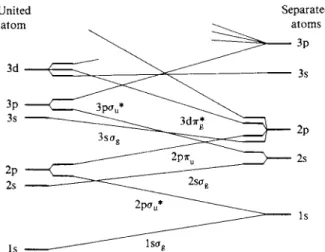
The various molecular orbitals can be described in other terms. It was noted earlier that lag goes over to ^(ls) for Η at large R and to ^(ls) for H e+ at zero R, while l au goes from 0(ls) for Η to ψ(2ρ) for H e+. Figure 18-7 summarizes these behaviors for a number of molecular orbitals for the general case of an A—A hydrogen-like molecule, the "united atom" being that resulting from the fusion of two A nuclei ( H e+ in the case of H2+) . Diagrams of this type are known as correlation diagrams.

A rule that we will not prove here is that states of the same orbital symmetry cannot cross. Thus a ae cannot cross another ag . A qualitative physical explanation is that at such a crossing one would have two states of the same symmetry and same

Separated atoms

FIG. 18-7. Correlation diagram showing how molecular orbital energies change with internuclear distance in an A—A-type molecule. (From C. A. Coulson, " Valence," 2nd ed. Oxford Univ. Press, London and New York, 1961.)

energy, and some linear combination of the states must exist such that one state is raised and the other lowered in energy. The effect is that such lines avoid each other in a correlation diagram.

Notice that in Fig. 18-7 the molecular orbitals are designated not as we have been doing u p to now, but rather in terms of the atomic orbital to which they go in the united atom. Thus our lag and l au have become l s ag and 2pau*.

(a) (b)

FIG. 18-8. Contour diagrams for normalized molecular orbitals ofH2+ with R = 2a0 . (a) lae (or lsag); (b) 1πα (or 2 px^{7 r}u^{) .} The small arrows mark the nuclear positions; the contours span about a tenfold range of φ value. [Adopted from D. R. Bates, K. Ledsham, and A. L. Stewart, Phil.

Trans. Roy. Soc. (London) A246, 215 (1953).]

Bonding overlap Antibonding overlap ss

(σ) sp

"end-on"

(σ) sp

"sideways"

nonbonding

"end-on" PP (o)

PP

"sideways"

(ΤΓ)

Pd

"sideways"

(π)

F I G . 1 8 - 9 . Sigma and pi bonding and antibonding orbitals. [From Β. N. Figgis, "Introduction to Ligand Fields." Copyright 1966, Wiley (Interscience), New York. Used with permission of John Wiley & Sons, Inc.]

This designation in terms of the united atom state is useful to spectroscopists and theoreticians. The physical chemist is more interested in the orbital designations for the separated atoms, since he visualizes the two as coming together to form the A—A bond. The third way of describing molecular orbitals is on such a basis. The

Ισε orbital goes over to ls orbitals of the separated atoms; it may be thought of qualitatively as the result of overlap between two ls atomic orbitals. Correspond­

ingly, as shown in Fig. 18-8(a), the lag molecular orbital has cylindrical symmetry around the internuclear axis (as, indeed, the designation σ indicates), and would be called lsag.

The l 7 ru orbital is degenerate, with one obeying a cos φ and the other a sin φ

function. For one, the electron density is a maximum at 0° and 180°, and for the other, at 90° and 270°. Figure 18-8(b) shows the electron density contours for one of these (in the xz plane) ; the orbital would look like a pair of sausages lying above and below the internuclear line. From the correlation diagram, we find that the* l 7 ru orbital goes over to 2 p * orbitals on the separated atoms. Conversely, it can be viewed as resulting from the overlap of two 2p.* atomic orbitals. Accordingly, we now designate it as 2 p * 7 ru or just as 2 ρ πα . The other of the pair would be 2py?ru . The above way of seeing how molecular orbitals are generated is summarized in Fig. 18-9 for several combinations. Note that the signs (or phases) of the atomic orbitals used are important. Bonding overlap occurs when the overlapping regions are of the same sign, and antibonding overlap when they are of opposite sign. It can happen that the like sign and opposite sign regions balance to give zero net overlap. Such a case is called nonbonding. An example is the sp sideways bonding in Fig. 18-9.

18-4 Variation Method for Obtaining Molecular Orbitals

The variation method may be used to obtain approximate molecular orbital functions and energies. We construct an approximate wave function for the mole­

cule as a whole and write for a diatomic molecule

Φ = αφΑ + άφΒ = η(φΑ + λφΒ), (18-22) where η is a normalization factor and λ is an adjustable constant. The φΑ and φΒ

are suitable combinations of atomic orbitals on atoms A and B. This means of constructing φ is known as the LCAO approximation—linear combination of atomic orbitals. If the molecule is H2+ or H2, the Is orbitals of each hydrogen atom are the appropriate ones to use in obtaining the lowest-energy molecular orbitals (and in this case λ = ± 1 since the atoms are the same).

In general, φΑ and φΒ are not the same functions and the variation method is used to find an optimum value for the mixing coefficient λ. On doing this (and eliminating λ), we find

(E - EA)(E - EB) = (HAB - ESAB)\ (18-23) where EA and EB are the energies associated with the atomic orbitals (and are

equal to the integrals J </rA*H^A and j φΒ *H</fB dr, also called Coulomb integrals, although not the same ones as used in the valence bond method (the e 2jr12 term is absent) ; Ε is the energy of the best molecular orbital function φ. The quantity HAB is the integral J φΑ*ΟφΒ dr (also called a resonance integral, although again not the same one described in Section 18-2), and . SAB is the overlap integral J ΦΑ*ΦΒ dr, which is the same as the S integral of Section 18-2. Equation (18-23) has two roots, so that two combinations of φΑ and φΒ in Eq. (18-22) are indicated, a bonding and an antibonding one. In the case of H2+, these were the l s ^ and l s au* molecular orbitals.

As noted in the preceding section, not any combination of atomic orbitals will lead to bonding. The φΑ and φΒ must have the same symmetry relative to the bond­

ing axis. Thus if ζ is the bonding axis and we attempt to use an s and a p* orbital for φΑ and φΒ , the molecular orbital energy turns out to be just EA or EB; that is, no interaction results. This is a consequence of the fact that HAB and SAB are separable into integrals of equal magnitude and opposite sign and are therefore zero (note Fig. 18-9). As noted earlier, the situation is known as nonbonding. Pairs of orbitals which behave this way are also called orthogonal.

18-5 Molecular Orbital Energy Levels for Diatomic Molecules

Molecular orbitals for A—A-type molecules, where A is other than hydrogen, are qualitatively the same as for H2 + . The energies are affected, however, by the screen­

ing of the nuclear charge by the inner electrons and a Ze ff must be used. At a more elaborate level, self-consistent field (Section 16-CN-3) wave functions are used as the basis, and some very extensive calculations have been made. Qualitatively, however, we order the molecular orbitals in sequence of increasing energy and pro-

Molecular

Atom A orbital Atom Β

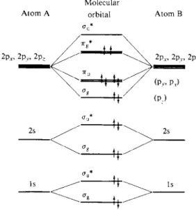
F I G . 1 8 - 1 0 . Molecular orbital energy level diagram for 02.

ceed to populate them with the requisite number of electrons. Each orbital can hold a pair of electrons, with spins opposed, and the set of molecular orbitals is filled with pairs of electrons.

Figure 18-10 shows a qualitative molecular orbital energy level diagram appro­

priate for light elements. Following the building-up procedure, the H2 molecule has the configuration ( l s ag)2 and H e2 would have (lsffg)2(lsau*)2. In this last case there are two electrons in a bonding and two in a nonbonding orbital; the net situation is equivalent to one of essentially no bonding, as observed—He2 is not a stable molecule. However, an electronically excited H e2 molecule of configuration (lsag)2(lsau*)(2stfg) should have a net bonding, as is actually found to be the case.

Moving to second-row elements of the periodic table, Li2 has the configuration (2sag)2 (the inner electrons make no net contribution and therefore are ignored);

the molecule should exist, and does—its dissociation energy is about 1 eV. The Be2 molecule should be like He2—it is, in fact, not known. The next elements now involve 2p orbitals, which may be either 2ρσ or 2 ρ π in type.

The cases of N2 and 02 are especially interesting. The first has the configuration (2sag)2 ( 2 s au* )2 (2ρσ)2 (2p7ru)4. There are two 2p7ru orbitals of equal energy (or degenerate) so that four electrons may be accommodated; they are bonding, so N2 has a net of six bonding electrons, corresponding to the triple bond in the usual formula. The Oa molecule is (2sag)2 (2sau*)2 (2pag)2(2p7ru)4 (2p77g)2 and therefore has a net of four bonding electrons, corresponding to a double bond (2p7Tg being antibonding). Since the 2p7rg set is only half filled, the pair of electrons in it are not required to pair their spin and, by Hund's rule (see Section 16-ST-l), do not. As a consequence, the ground state of oxygen is a paramagnetic one, called *Σ, corresponding to two unpaired electrons. The situation is illustrated in Fig. 18-10.

These examples illustrate one important application of the molecular orbital approach. If one neglects interelectronic repulsions, a set of molecular orbital states is obtained into which the proper number of electrons are fed. One thus obtains a good qualitative understanding of the geometry of the filled orbitals

18-6 Triatomic Molecules. Walsh Diagrams

The bonding in triatomic and in MXn-type molecules may be treated in terms of atomic orbitals suitably hybridized so as to give a maximum overlap in the bonding directions. The use of group theory for determining what combinations of orbitals should be hybridized for the central atom is discussed in a previous chapter (Section 17-7) and the bonding can then be treated in terms of molecular orbitals formed between the hybrid orbital and an orbital on each of the X atoms.

While absolute bonding energies are very difficult to calculate, it is possible to reach qualitative conclusions about how the energies of the various molecular orbitals vary with geometry. The simplest case is that of the M H2 molecule.

If it is linear, the molecular orbitals may be of the sigma type, formed between the ls hydrogen atomic orbitals and the s py hybrid orbital of the M atom (v being the H — M — H axis). One then obtains a pair of orbitals ag and ση, the first being lower in energy. The remaining p* and p2 orbitals of M are pi in type and nonbonding; the molecular orbital is designated TTU and is twofold degenerate.

Consider next the situation if the H—M —H angle is 90°. The molecule is now C2V in symmetry, with irreducible representations A1, A2, ΒΎ, and B2. A sigma M —H bond can be formed by the overlap of a pure ρ orbital on M with the ls orbital on H, and the two M — H bonds would then involve the p2 and py M orbitals. These are equivalent, however, and the corresponding molecular orbitals are formed by taking the in-phase and the out-of-phase combinations of the two localized orbitals. The symmetry properties of these two molecular orbitals identify them as belonging to the ax and b2 irreducible representations. (It is customary to use lower case letters in giving the IR to which a molecular orbital belongs.) The remaining p* orbital is nonbonding and belongs to the b1 irreducible

representation. Finally, the s orbital on M is also nonbonding and has the symmetry designation ax.

One may now assemble the correlation diagram shown in Fig. 18-11 [see Walsh (1953)]. As the H — M — H angle is increased from 90° the ax and b2 bonding orbitals must eventually become the ag and au orbitals, respectively, of the linear molecule. At the same time the binding energy of the orbitals must increase—one way of seeing this is that increasing s character develops in the bonds and sp hybrid orbitals give rise to a stronger bond than do those for pure p. Figure 18-11 is obtained from such considerations plus the no-crossing rule mentioned in connection with Fig. 18-7.

and, as in the case of Oa, can predict cases of paramagnetism. In addition, it is easy to describe excited states as configurations in which one or more electrons are promoted to higher-energy molecular orbitals. This aspect will be discussed further in Chapter 19.

In the case of A—Β molecules, there is no longer a center of symmetry and the g and u designations do not apply to the molecular orbitals. Also, since ^A( l s ) does not have the same energy as 0B(ls), etc., the atomic orbital positions in a diagram such as Fig. 8-10 will lie on different energy scales. This can result in some shifting in the relative positions of the various molecular orbitals, to be determined by calculation. Given the molecular orbital energy level sequence, however, the pro­

cedure is as before—one adds the requisite number of electrons, in pairs, and beginning with the lowest-energy orbital.

While the energy scale is qualitative, the figure does allow some conclusions as to molecular geometry. A given M H2 molecule will have a certain number of outer electrons, to be placed in the lowest possible molecular orbitals; each orbital has a capacity of two electrons (with spins opposed). A molecule such as BeH2 or H g H2 has four outer electrons, so that the ag and ση orbitals are just filled.

The linear configuration is the lowest-energy one, so these molecules are predicted to be linear. On the other hand, M H2 molecules having five, six, seven, or eight valence electrons should be bent. This is the case with H20 , for example. The actual angle cannot be obtained from Fig. 18-11; it would be determined as the optimum compromise between the opposite trends of the ax (s) orbital and the ax and bx orbitals. Similarly, the molecule C H2 should be bent, but less so in that excited state which has an electron promoted to the bx orbital (why?). Walsh diagrams thus also allow predictions of how molecular geometry should change in excited states (see also Section 19-CN-2); more complex diagrams are available for M A2 (Α Φ Η) molecules, and so on.

18-7 Polyatomic Molecules. The Hiickel Method

A number of rather approximate, semiempirical methods have been developed in an effort to calculate or at least to organize in a reasonable way the experimental properties of molecules in which pi bonding seems to be present. A rather useful and widely used approach is the following.

A set of pi-bonding molecular orbitals is developed by using the variation method and taking φ to be a linear combination of wave functions which are of symmetry suitable for such bonding:

φ = αφ1 + bφ2 + οφζ · (18-24)

The condition for the optimum set of coefficients a, b, c, etc., is given by the secular equation, Eq. (16-104). The problem, of course, is to evaluate the integrals!

A. The Huckel Approximations

We will now solve Eq. (16-104) by making some rather drastic-appearing approxi­

mations. In the case of molecules which are held together by a framework of sigma bonds but which also have available pi bonding orbitals, a set of pi-bonding molecular orbitals can be developed by taking φ1, φ2, and so on to be the wave functions on each atom which are of symmetry suitable for pi bonding. The usual situation is one of a chain or ring of carbon atoms, and each φ is then a carbon ρ orbital perpendicular to the sigma bond. In ethylene, for example, the

H

H '

;c-c:

H

Ή

sigma bonding framework might be regarded as provided by s p2 hybrid bonds of each carbon atom. The remaining carbon ρ orbitals then overlap to give some pi bonding,

Η / θ ® \ H

In this case, which is typical, one then takes φ1^{, φ}2, and so on to be the same, that is, one ρ orbital per carbon. The specific further approximation made in the treatment by E. Huckel is then to assume that all integrals of the type Hu ^are the same and equal to a constant a; as mentioned earlier (Section 18-4), these are called Coulomb integrals. Integrals of the type Hu, called resonance integrals, are taken to be the same and equal to a constant β if / and j refer to adjacent atoms and to be zero otherwise. The atomic ρ orbitals are assumed to be normalized so that all Su = 1 ; there is complete neglect of overlap integrals, that is, all Sif ^are taken to be zero.

Equation (18-8), which applies to ethylene, then becomes (a-E) β

β (ce -Ε) = 0. (18-25)

F o r butadiene, H2C = C H — C H = C H2, the secular equation is (H^-ES^) (#12

( # 1 2 ~ ^ 1 2 ) ( # 2 2 ( # 1 3 ~ ^ 1 3 ) ( # 2 3

(H1A-ES14) (#24

ES12) ( # 1 3 - ^ 1 3 ) ( # 1 4 - ^ 1 4 )

ES22⁾ ( # 2 3 - ^ 2 3 ) ( # 2 4 - ^ 2 4 )

ES23) ( # 3 3 — ESS3) ( #34 — £ £ 3 4 )

^ 2 4 ) ( # 3 4 - ^ 3 4 ) ( # 4 4 - ^ 4 4 )

(a-E) β 0 0 β (ce-Ε) β 0 0 β (ce- Ε) β 0 0 β (ce-Ε)

= 0

= 0

(18-26)

~2β ^k

+β

+2β

(0.62/3)

Π

(1.62/3)

— C H 2 C^H^

t t

t l H

o

T 3

(CH)„

cyclic

F I G . 1 8 - 1 2 . Pi electron molecular orbital levels according to the Huckel model.

since, for example, Hu = 0 and £14 = 0, and so on. The solution to the ethylene secular equation is simply Ε = a + β and Ε = a — β [note Eqs. (18-11) and (18-12)].

Since a corresponds to the energy for the isolated atom, it is customary to take this as a point of reference, and the solutions for ethylene are as shown in Fig. 18-12.

The β integrals are negative in value, so that oc + β is the lower lying of the two.

There are two pi electrons to place and since they may occupy the same level if their spins are opposed, this is the assumed configuration for ethylene.

The solutions for butadiene are+

oc + K V5 + 1)β, a + K V5 - 1)β, K V 5- l ) j 8 , a^{_ K V 5}+ l ) j 8 . There are now four electrons to place and these fill the first two levels in pairs.

In the case of cyclobutadiene, integrals such as Hu are equal to β since these atoms are now adjacent; solution of the resulting equation gives α + 2β, oc, oc, and α — 2β. That is, there are two solutions with Ε = a; such a case is called one of degeneracy. There are again four electrons to place and therefore two must go

+ Divide every row by β and let m = (α — Ε)/β, to give the determinant m 1 0 0

1 m 1 0 0 1 m l ' 0 0 1 m

which expands to m4 — 3m2 + 1 = 0. If now y = m2, the equation becomes y2 — 3y + 1 = 0, which is easily solved.

into the degenerate pair of E= a levels. As noted in Section 18-5, an empirical rule of spectroscopy is that it takes energy to pair electrons, that is, to oppose their spins. The rule, known as Hund's rule, then calls for the two electrons to have their spins parallel. Cyclobutadiene should thus be a paramagnetic molecule with magnetic susceptibility corresponding to two unpaired electrons (Sec­

tion 3-ST-2).

In terms of the assumptions made, the energy of the pi orbitals would be just not, where η is the number of pi electrons, if no mixing or linear combination is used. The difference between this and the calculated energy is then the stabilization (or destabilization) due to molecular orbital formation; it is called the delocalization energy. This energy is —2β for ethylene and —4ΛΊβ for butadiene. The fact that this last is more than twice the value for ethylene suggests that in butadiene the molecular orbitals extend over the whole molecule, or that one does not simply have two connected ethylene units, as the usual formula H2C = C H — C H = C H2 might suggest. The delocalization energy for cyclobutadiene is 4β9 however, or just that of two ethylenes, which indicates that the ring structure provides no added stability. Cyclobutadiene has in fact been very difficult to synthesize, its existence seems at best to be transient, and the Hùcke l treatmen t doe s indicat e that th e molecul e shoul d b e unstabl e sinc e n o extr a delocalizatio n energ y i s present t o offse t th e strai n energ y o f coercin g th e sigm a bon d framewor k t o a four-membered ring .

β . Evaluation of the Resonance Integral β

The integrals Hi5 can be estimated theoretically, but it is relatively easy to evaluate β experimentally, and this is what is usually done. For example, the heat of hydrogénation of ethylene is 32.8 kcal m o l e-1 and were butadiene just two noninteracting ethylene units, the value should be 65.6 kcal m o l e- 1. The observed value is 57.1, so butadiene appears to be more stable than expected by 8.5 kcal m o l e- 1. The extra delocalization energy from the Huckel treatment is 0.47/3, which makes β = \% kcal m o l e- 1.

The case of benzene is an important one, and solution of the appropriate secular equation gives the molecular orbital levels shown in Fig. 18-12; the pi bonding energy is 8/3, as compared to 6β were benzene simply three ethylenes linked together. The extra stabilization is then 2β. Either from bond energies (Section 5-ST-l) or comparison of heats of hydrogénation of ethylene and of benzene, the experimental delocalization energy is 35-40 kcal m o l e- 1, again giving a β value of 18-20 kcal m o l e- 1.

If β is taken to be generally about 18-20 kcal m o l e-1 for carbon-carbon bonded systems, then application of the Huckel approach allows at least approximate delocalization energies to be calculated for a variety of linear and cyclic molecules.

Included are rings of the type C5H5 and C5H5-, C7H7, and other unstable species.

The method has been extended to heterocyclic rings, to peroxo rings (where each carbon atom of the ring is also bonded to an oxygen), and so forth.

One may also estimate the energy to put a molecule in an excited state. That is, the lowest-lying electronic excited state is very likely that corresponding to promoting an electron to the first unoccupied pi molecular orbital. This energy should then be 2/3 for ethylene, 1.24/3 for butadiene, and so on. As shown in Fig. 18-13, a plot of the frequency of the first absorption band against the cal-

70,000

0.4 0.6 0.8 1.0 1.2 1.4 1.6 1.8 2.0 2.2

β

F I G . 1 8 - 1 3 . Spectroscopic evaluation of β (frequency of the first π —> π * transition of various polyenes against energy in units of β). (From A. Streitweiser, Jr., "Molecular Orbital Theory for

Organic Chemists." Copyright 1961, Wiley, New York. Used with permission of John Wiley &

Sons, Inc.)

culated energy in units of β is reasonably linear. The slope yields β = 60 kcal m o l e- 1.

This last value for β is, of course, quite different from that of about 20 kcal m o l e-1 from the thermochemical data. The probable reason is that in the thermo­

chemical approach one is comparing actual heats of hydrogénation with those for a hypothetical structure of alternate single and double bonds, each of its natural bond length. The reference structure for, say, benzene is thus

It is first necessary to stretch the double bonds to the structure

before considering derealization energy. The energy for this bond length changing has been estimated to be about 37 kcal m o l e- 1. The experimental derealization energy of about 40 kcal m o l e-1 thus represents an excess over the 37 kcal m o l e-1 for bond distortion, so that the corrected experimental value becomes about 77 kcal m o l e- 1, making β about 38 kcal m o l e- 1, or considerably closer to the spectroscopic value.

The discussion illustrates the fact that thermochemical values include various contributions, such as bond length changes, not present in the spectroscopic values. The consequence is that β values are best used only in the context of the manner in which they were obtained.

C. Huckel Wave Functions

The coefficient s o f a Hùcke l molecula r orbita l

Φο = €\όΦι + c2 ^ 2 + ε^Ψζ + ··" » (18-27) where φ1, φ2,... are the atomic orbitals, may be obtained as follows. If we take

the molecular orbital <£'s to be normalized, then

j φΐ*φι dr = 1 = 4 j dr + 4 j φ2*φ2 dr + ··· ,

all the cross terms J* ψΐ*ψί dr vanishing if the φ functions are orthogonal. If the functions are also normalized, then the remaining integrals are unity, so we have

4 + 4 + 4 + - = L (18-28) W e find additional relationships between the c{j as follows. The precursor

equation to Eq. (18-3), Eq. (16-30), is Ηφ}- = Εφ,·, or ( Η - Ε)φ5 = 0. Suppose we are considering φχ ; then substitution of φλ = €λ1φλ + ο21φ2 + ··· , multi­

plication by ι/^*, and integration gives

cu J>i*(H - Ε)φχ dr + c21 JVCH - Ε)φ2 dr + ... = 0,

or, on insertion of the Hûcke l assumption s regardin g Hn an d H12,

cu( a - € ) + €21β = 0 (18-29)

(assuming only atoms 1 and 2 are adjacent). Similar equations follow for the other coefficients on repeating the operation with φ2*9 ... .

Thus in the case of butadiene, Eq. (18-29) applies, and since for the lowest energy state Ε = a + %(V5 + 1)β, the result is c21 = i(V5 + l ) cn . Pursuing the procedure, we find that c31 = i(V5 + 1) c41 and cn = c4 1. All the may

(c) (d)

F I G . 18-14. Huckel molecular orbitals for butadiene.

then be expressed in terms of cn , and insertion of these relationships into Eq. (18-28) gives cn = 0.37; it then follows that c41 = 0.37, c21 = c31 = 0.60.

Thus for the lowest molecular orbital φλ = 0.37(0! + 04) + O.6O(02 + 03). The whole process can then be repeated for the other three molecular orbital states.

The results are summarized in Fig. 18-14, which shows schematically how φΐ 9φ2, φζ, and 04 contribute to each molecular orbital.

D. Application of Group Theory to Carbon Rings

Somewhat of a shortcut may be taken in evaluating the 0's if the carbon chain forms a ring. In the case of a six-membered ring (benzene) the molecular point group is D6h . We can then find the traces for the reducible representation generated by a set of six ρπ orbitals and then the irreducible representations to which the set corresponds. Each irreducible representation will have the symmetry of one of the molecular orbital energy states.

If we only want to know signs of the ρπ orbitals for each solution, then it is only necessary to look at the symmetry of each irreducible representation with respect to the C6n operations. It is therefore easier to fall back to the C6v group, for which the irreducible representations are half in number, but otherwise the same as far as the traces for the Cn operations. In C6 V, the traces for the set of six ρπ bonds are

Ε 2 C6 2 C3 C2 3 σν 3σ(ΐ

ρπ 6 0 0 0 2 0

Application of Eq. (17-16) gives Γ6πΡ = Λλ + Bx + E1 + E2. The Αλ IR is totally symmetric, and so must correspond to the ρπ orbitals having all plus lobes on one side (and all minus lobes on the other). Thus

φ, = ( 1 / V 6 X 0 ! + 02 + 03 + 04 + 05 + 0e);

the factor 1/V6 is a normalization coefficient. The Bx IR is antisymmetric to the operation C6 (and C65) and this as well as its other properties means that the signs of the 0's must alternate. Then 02 = ( 1 / V 6 X 0 ! — 02 + 03 — 04 + 05 — 06). The E1 and E2 IR are two-dimensional, and a somewhat more lengthy procedure is needed to find the coefficients of the 0's; only the results are given here:

E l

' ^

E<2 · 05 = (201 — 02 + 204 — 05 — 06)>

06 = \ (02 — 03 + 04 — 0δ)·

The various φ functions correspond to sets of standing molecular orbital waves as illustrated in Fig. 18-15.

Φι Φι

F I G . 1 8 - 1 5 . Hùckel molecu- lar orbitals for benzene.

£. The 4x + 2 Rule. Bonding, Nonbonding, and Antibonding Molecular Orbitals

The Hùcke l treatmen t lead s t o a simpl e rul e whic h state s tha t a rin g ( C H ) n will hav e aromati c characte r i f η = 4x + 2, χ being an integer. The qualitative reasoning behind this rule is the following. Referring to Fig. 18-12, molecular orbitals lower in energy than a are said to be bonding since electrons placed in them are lower in potential energy than in the absence of the molecular orbital formation. Orbitals equal in energy to α are said to be nonbonding, or neutral in this respect, and those lying above α are then antibonding. On placing η electrons in the set of molecular orbitals, the molecule is stabilized as a result of molecular orbital formation, that is, of delocalizing the atomic orbitals, to the extent that the total energy is less than not.

It is clearly undesirable to have to place electrons in nonbonding or antibonding orbitals. If (CH)n is to be aromatic or extra stable, it is first of all necessary that η be even; since there are η pi electrons, the molecule would otherwise be a free radical. Second, the molecular orbital energy level scheme must be such that all η electrons can be accommodated, in pairs, in bonding orbitals. As may be inferred from Fig. 18-12 the pattern of molecular orbitals given by the Huckel treatment for η even is one of a single lowest-lying orbital and a single highest-lying one, and then one or more sets of doubly degenerate orbitals. That is, there will be η — 2 degenerate orbitals occurring in (n — 2)/2 pairs. If (n — 2)/2 is an odd number, then one of the sets of degenerate orbitals will be nonbonding, as in the case of ( C H )4. Since the n/2 pairs of electrons must just half fill the set of orbitals, this means that two must be nonbonding. To avoid this situation, (n — 2)/2 must be an even number, or 2x, where χ is an integer. It then follows that η = Ax + 2 if all electrons are to be paired and all to be in bonding orbitals.

According to this rule, C4H4 is not aromatic, C6H6 is, C8C8 is not, C1 0H10 is, and so on. This is the experimental observation.

COMMENTARY AND NOTES 18-CN-l Comparison of the Valence Bond

and Molecular Orbital Methods

The valence bond (VB) and molecular orbital (MO) methods are the two principal ones of wave mechanics for dealing with molecules. Both use the variation method, but with different procedures for obtaining the approximate wave function, φ.

In the VB method, one starts with two atoms, each with its bonding electron, but recognizes that electron 1 may be on atom A and electron 2 on atom B, or vice versa. The approximate wave function whose coefficients are to be optimized is thus

Φνη = αφΑ(1)φΒ(2) + άφΑ(2)φΒ(1). (18-30) In the M O method, one starts with two atoms, sans electrons, and writes as the

approximate wave function

Φι = *I0AO) + *I*B(1). (18-31)

That is, electron 1, the first electron, is taken to move in the field of the two nuclei.

If we are to add a second electron to the same molecular orbital, we have

02 = α2φΑ(2) + ά2φΒ(2). (18-32)

The wave function for both electrons is just the product φχφ2 (neglecting inter- electronic repulsion), so that

0MO = 0Ι#20ΑΟ)0Α(2) + άφ2φΒ(1)φΒ(2)

+ αφ2φΑ(1)φΒ(2) + αΑ0Α(2)0Β(1). (18-33) The first two terms on the right correspond to both electrons being on atom A or

both on atom B, or to the configurations A ~ Β + and A+Β ~, while the last two terms are essentially the same as 0VB · The M O formulation thus tends to give emphasis to ionic configurations and, in fact, to overemphasize them. The VB method underestimates ionic contributions, on the other hand, and these are usually added so as to improve the results, as in Eq. (18-18).

For the chemist, however, the M O description generally gives a better picture of molecular bonding. It also provides a n easy basis for the qualitative discussion of molecular excited states and, as in the Hûcke l treatment , o f delocalize d bonding .

The M O metho d ha s bee n applie d extensivel y t o smal l molecules , wit h th e hel p of a greatl y simplifyin g an d importan t approximation . Th e differentia l overla p between tw o atomi c function s 0fc an d φι is defined as the probability of finding an electron i in a volume element common to 0fc and φι and is represented by

ski = 0fcO'WO-

The approximation is that Skl is zero unless k is equal to /. The abbreviated name for the procedure is CNDO (complete neglect of differential overlap).

The C N D O approximation allows whole categories of integrals in the secular equation to be made zero or unity. The situation is reminiscent of that of the Hûcke l method, excep t tha t sigm a a s wel l a s p i bondin g i s calculated . Th e remainin g integrals ar e stil l formidable , an d t o hel p matters , th e hydrogen-lik e atomi c wav e

functions are approximated by Gaussian-type functions which are similar graphi­

cally but much more tractable mathematically.

The C N D O approach, proposed by Pople, Santry, and Segal (1965), has led to a whole spectrum of related calculational procedures. As a result we now have fairly good calculated bond lengths, bond energies, and dipole moments for a variety of small molecules. The method is sufficiently reliable to be used in the prediction of properties of otherwise unaccessible species such as chemical reaction intermediates.

SPECIAL TOPICS

18-ST-l Ligand Field Molecular Orbital Diagrams

The electronic structure of an octahedral transition metal coordination compound was approached in Section 17-CN-l in terms of the perturbing effect of the octa­

hedral field on a set of five d electrons. As shown in Fig. 17-15, the fivefold degener­

acy is partially removed, to give a set of t2g orbitals and one of eg orbitals, the former being lower in energy. One could then calculate crystal field stabilization energies by placing the requisite number of metal d electrons in these orbital sets.

The purely electrostatic crystal field picture has now given way largely to what is called ligand field theory. Perhaps the main change is that bonding is now recognized as occurring between the ligands and the central metal ion. On making up a linear combination of six ligand sigma bonding orbitals and the s, p, dX2_y2, and d?2 metal orbitals, one, as usual, obtains a bonding and an antibonding set.

* 1 *

F I G . 1 8 - 1 6 . Sigma bonding molecular orbital diagram for an octahedral transition metal complex.

This is illustrated in Fig. 18-16; the asterisks denote antibonding orbitals. The t2g orbitals are not suited for sigma bonding and therefore do not participate, that is, are nonbonding. Since a set of bonds for the whole molecule is involved, Fig. 18-16 is usually called a molecular orbital diagram. The small letters a, t2g , and so on are used as a reminder that the energy levels are those which a single electron could have. The bonding levels are, of course, actually occupied by 12 electrons, two from each ligand, and, in the case chosen here, Cr(III), the t2g set is occupied by three electrons, thought of as belonging to the central metal ion.

A point that should be mentioned is that the set of nonbonding metal electrons also has a symmetry designation, in this case *A2g . The superscript gives the spin multiplicity or number of energetically equivalent ways in which the spin S = f may combine with the orbital angular momentum (see Section 16-ST-l). In the case of Co(III) complexes, the symmetry designation of the set of six t2g non- bonding metal electrons is 1Alg .

Returning to the figure, the quantity Δ, now called the ligand field strength, is the separation between the t2g and the eg* sets—it functions in much the same way as in crystal field theory. Its value, however, is now treated as primarily dependent on the strength of the bonding rather than as arising from the octahedrally disposed charges of crystal field theory. We find, for example, that various ligands produce an effective ligand field strength in the order N H3 > H20 > OH~ > CI" > Br~.

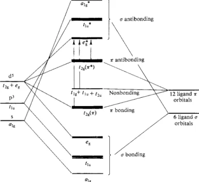
Recalling Section 17-CN-l, the di; or t2g set of metal orbitals is suited for pi bonding, the set of 12 pi bonding ligand orbitals also generating the tlg , rlu , and t2u representations in Oh symmetry. One may next obtain bonding and corre­

sponding antibonding combinations of pi symmetry orbitals to give the yet more complete molecular orbital diagram shown in Fig. 18-17. The pi bonding orbitals

FIG. 18-17. Same as Fig. 18-16, but also showing pi bonding.

can hold up to six electrons and the nonbonding ones up to 18. It is not easy to determine the actual degree of pi bonding in a complex ion, and diagrams such as this one are necessarily rather schematic in nature. It is clear, however, that the energy separation Δ between the highest occupied level and the lowest unoccu­

pied level must in reality be a rather complicated quantity.

GENERAL REFERENCES

ADAMSON, A. W. (1969). "Understanding Physical Chemistry," 2nd ed., Chapter 21. Benjamin, New York.

COTTON, F. A. (1963). "Chemical Applications of Group Theory." Wiley (Interscience), New York.

COULSON, C. A. (1961). "Valence," 2nd ed. Oxford Univ. Press, London and New York.

DAUDEL, R. LEFEBVRE, R., AND MOSER, C. (1959). "Quantum Chemistry." Wiley (Interscience), New York.

FIGGIS, Β. N. (1966). "Introduction to Ligand Fields." Wiley (Interscience), New York.

EYRING, H., WALTER, J., AND KIMBALL, G. E. (1960). "Quantum Chemistry." Wiley, New York.

HALL, L. H. (1969). "Group Theory and Symmetry in Chemistry." McGraw-Hill, New York.

HANNA, M. W. (1969). "Quantum Mechanics in Chemistry," 2nd ed. Benjamin, New York.

OFFENHARTZ, P. O'D. (1970). "Atomic and Molecular Orbital Theory." McGraw-Hill, New York.

PITZER K . S. (1953). "Quantum Chemistry." Prentice-Hall, Englewood Cliffs, New Jersey.

SEGAL, G. A. (1977). "Semiempirical Methods of Electronic Structure Calculation," Part A.

Plenum Press, New York.

STREITWEISER, Α., JR. (1961). "Molecular Orbital Theory for Organic Chemists." Wiley, New York.

CITED REFERENCES

ADAMSON, A. W. (1969). "Understanding Physical Chemistry," 2nd ed. Benjamin, New York.

COTTON, F. A. (1963). "Chemical Applications of Group Theory." Wiley, New York.

LINNETT, J. W. (1964). "The Electronic Structure of Molecules." Methuen, New York.

MULLIKEN, R , RIEKE, C. Α . , ORLOFF, D., AND ORLOFF, H. (1949). J. Chem. Phys. 1 7 , 1248.

POPLE, J. Α . , SANTRY, D . P . , AND SEGAL, G. A . (1965). / . Chem. Phys. 4 3 , S192.

WALSH, A. D. (1953). / . Chem. Soc. 1 9 5 3 , 2260, 2266.

EXERCISES

1 8 - 1 Verify Eq. (18-10).

1 8 - 2 Explain why the lag wave function reaches a maximum value of 0.4 in Fig. 18-4(a), and four times this, or 1.6, in Fig. 18-4(c). (The reference cited will be helpful.)

1 8 - 3 Explain why, in Fig. 18-5, the lag molecular orbital approaches the limits —4 and — 1, and why the lau molecular orbital approaches the limits —1 and —1.

1 8 - 4 Sketch, in the manner of Fig. 18-9, bonding, antibonding, and nonbonding overlap situations involving an s and a d orbital.

1 8 - 5 Consider the molecule C2. (a) Should it be stable? (b) What should the bond order be?

(c) Should it be diamagnetic or paramagnetic ?

Ans. (a) Yes. (b) 2. (c) Paramagnetic.