International Journal of Fuzzy Systems
OUTLIER DETECTION ALGORITHMS OVER FUZZY DATA WITH WEIGHTED LEAST SQUARES
--Manuscript Draft--
Manuscript Number: IJFS-D-19-00829R2
Full Title: OUTLIER DETECTION ALGORITHMS OVER FUZZY DATA WITH WEIGHTED
LEAST SQUARES
Article Type: S.I. : Fuzzy models for Business Analytics Funding Information: Hungarian National Research,
Development and Innovation Office (NKFIH)
(129528, KK)
Prof. Krasimir Kolev
Higher Education Institutional Excellence Programme of the Ministry of Human Capacities in Hungary
(Molecular Biology thematic programme of Semmelweis University (KK))
Prof. Krasimir Kolev
University of Tasmania
(RT.112222) Prof. Kiril Tenekedjiev
Abstract: Abstract In the classical leave-one-out procedure for outlier detection in regression analysis, we exclude an observation, then construct a model on the remaining data. If the difference between predicted and observed value is high we declare this value an outlier. As a rule, those procedures utilize single comparison testing. The problem becomes much harder when the observations can be associated with a given degree of membership to an underlying population and the outlier detection should be generalized to operate over fuzzy data. We present a new approach for outlier that operates over fuzzy data using two inter-related algorithms. Due to the way outliers enter the observation sample, they may be of various order of magnitude. To account for this, we divided the outlier detection procedure into cycles. Furthermore, each cycle consists of two phases. In Phase 1 we apply a leave-one-out procedure for each non- outlier in the data set. In Phase 2, all previously declared outliers are subjected to Benjamini-Hochberg step-up multiple testing procedure controlling the false discovery rate, and the non-confirmed outliers can return to the data set. Finally, we construct a regression model over the resulting set of non-outliers. In that way we ensure that a reliable and high-quality regression model is obtained in Phase 1 because the leave- one-out procedure comparatively easily purges the dubious observations due to the single comparison testing. In the same time, the confirmation of the outlier status in relation to the newly obtained high-quality regression model is much harder due to the multiple testing procedure applied hence only the true outliers remain outside the data sample. The two phases in each cycle are a good trade-off between the desire to construct a high-quality model (i.e. over informative data points) and the desire to use as much data points as possible (thus leaving as much observations as possible in the data sample). The number of cycles is user-defined, but the procedures can finalize the analysis in case a cycle with no new outliers is detected. We offer one illustrative example and two other practical case studies (from real-life thrombosis studies) that demonstrate the application and strengths of our algorithms. In the concluding section, we discuss several limitations of our approach and also offer directions for future research.
Keywords: regression analysis, leave-one-out method, degree of membership, multiple testing, Benjamini-Hochberg step-up multiple testing, false-discovery rate
Highlights:
- We develop algorithms for outlier rejection over fuzzy samples using weighted least squares that operate in a given number of cycles
- Each cycle has two phases – use single testing leave-one-out procedure for initial purging of data, then confirm the previous outlier status with multiple testing
- We offer one illustrative example and two examples from a case study in thrombosis research to show the strength of our cycle-based approach
Corresponding Author: Natalia Nikolova, PhD
OUTLIER DETECTION ALGORITHMS OVER FUZZY DATA WITH WEIGHTED LEAST SQUARES
Natalia Nikolova1,2*, Rosa M. Rodríguez3, Mark Symes4, Daniela Toneva5, Krasimir Kolev6, Kiril Tenekedjiev7,8
1 Australian Maritime College, University of Tasmania 1 Maritime Way, Launceston
7250 TAS, Australia
E-mail: Natalia.Nikolova@utas.edu.au
* Corresponding author
2 Nikola Vaptsarov Naval Academy – Varna, Faculty of Engineering 73 Vasil Drumev Street
Varna 9026, Bulgaria
E-mail: natalianik@gmail.com
3 University of Jaén Campus las lagunillas s/n 23071, Jaén (Spain) E-mail: rmrodrig@ujaen.es
4 Australian Maritime College, University of Tasmania 1 Maritime Way, Launceston
7250 TAS, Australia
E-mail: Mark.Symes@utas.edu.au
5 Technical University – Varna
Faculty of Marine Sciences and Ecology 10 Studentska Str., Varna 9010, Bulgaria E-mail: dtoneva@abv.bg
6 Department of Medical Biochemistry, Semmelweis University, 1085 Budapest, Üllői út 26., Hungary
E-mail: Kolev.Krasimir@med.semmelweis-univ.hu
7 Australian Maritime College, University of Tasmania 1 Maritime Way, Launceston
7250 TAS, Australia
E-mail: Kiril.Tenekedjiev@utas.edu.au
8 Nikola Vaptsarov Naval Academy – Varna, Faculty of Engineering 73 Vasil Drumev Street
Varna 9026, Bulgaria
E-mail: Kiril.Tenekedjiev@fulbrightmail.org
ORCID Nikolova: http://orcid.org/0000-0001-6160-6282 ORCID Rodriguez: https://orcid.org/0000-0002-1736-8915 ORCID Symes: https://orcid.org/0000-0003-2241-4995 ORCID Toneva: https://orcid.org/0000-0003-1599-395X ORCID Kolev: https://orcid.org/0000-0002-5612-004X ORCID Tenekedjiev: https://orcid.org/0000-0003-3549-0671
Abstract In the classical leave-one-out procedure for outlier detection in regression analysis, we exclude an observation, then construct a model on the remaining data. If the difference between predicted and observed value is high we declare this value an outlier. As a rule, those procedures utilize single comparison testing. The problem becomes much harder when the observations can be associated with a given degree of membership to an underlying population and the outlier detection should be generalized to operate over fuzzy data. We present a new approach for outlier that operates over fuzzy data using two inter-related algorithms. Due to the way outliers enter the observation sample, they may be of various order of magnitude. To account for this, we divided the outlier detection procedure into cycles. Furthermore, each cycle consists of two phases. In Phase 1 we apply a leave-one-out procedure for each non-outlier in the data set. In Phase 2, all previously declared outliers are subjected to Benjamini-Hochberg step-up multiple testing procedure controlling the false discovery rate, and the non-confirmed outliers can return to the data set. Finally, we construct a regression model over the resulting set of non-outliers. In that way we ensure that a reliable and high-quality regression model is obtained in Phase 1 because the leave-one-out procedure comparatively easily purges the dubious observations due to the single comparison testing. In the same time, the confirmation of the outlier status in relation to the newly obtained high-quality 1
2 3 4 5 6 7 8 9 10 11 12 13 14 15 16 17 18 19 20 21 22 23 24 25 26 27 28 29 30 31 32 33 34 35 36 37 38 39 40 41 42 43 44 45 46 47 48 49 50 51 52 53 54 55 56 57 58 59 60 61 62
regression model is much harder due to the multiple testing procedure applied hence only the true outliers remain outside the data sample. The two phases in each cycle are a good trade-off between the desire to construct a high-quality model (i.e. over informative data points) and the desire to use as much data points as possible (thus leaving as much observations as possible in the data sample). The number of cycles is user-defined, but the procedures can finalize the analysis in case a cycle with no new outliers is detected. We offer one illustrative example and two other practical case studies (from real- life thrombosis studies) that demonstrate the application and strengths of our algorithms. In the concluding section, we discuss several limitations of our approach and also offer directions for future research.
Keywords: regression analysis, leave-one-out method, degree of membership, multiple testing, Benjamini-Hochberg step-up multiple testing, false-discovery rate
Highlights:
- We develop algorithms for outlier rejection over fuzzy samples using weighted least squares that operate in a given number of cycles
- Each cycle has two phases – use single testing leave-one-out procedure for initial purging of data, then confirm the previous outlier status with multiple testing
- We offer one illustrative example and two examples from a case study in thrombosis research to show the strength of our cycle-based approach
1. INTRODUCTION
Regression analysis aims to construct a linear model of a given process that relates to the relationship between a dependent (response) variable and one or more independent (explanatory, predictor) variables. Using that linear model, we can then make inferences regarding the process. Regression analysis serves for a wide range of predictions and forecasting, as well as to infer causal connections between the predictor and the response variables. The adequacy of the model benefits from a preliminary screening of the input sample for non-informative, misleading and/or erroneous data points, known as outliers [63]. In fact, the proper identification and rejection of outliers contributes to the quality of the regression model a lot more than the size of the input sample. Therefore, a procedure that associates with higher rejection rate (thus improving the quality of the sample) should be preferred over a procedure that has insufficient rejection of outliers (thus aiming to maintain somewhat larger sample size) [29].
Assume the initial sample has n observations. A typical procedure to detect an outlier is to exclude the i-th observation, construct a model on the remaining n–1 data points and measure the difference between the predicted and the observed value. If that difference is above a given threshold, the i-th observation is declared an outlier. Then n models test n hypotheses regarding the outlier status of an i-th observation. This procedure is in fact a leave-one-out (LOO) routine to test the performance of a model [46, 73]. It suffers from several drawbacks:
• the errors in the observations may vary significantly in scale and order of magnitude;
• once an observation is detected as an outlier it has no chance to return into the sample;
• all tests have the same significance level αcrit, yet multiple testing procedures require to change αcrit of the tests.
In a classical setup, we apply regression analysis over crisp data to study crisp relationships between the predictor and response variables [10]. Often, though, we deal with fuzzy data where the data points have some sort of an associated degree of membership to a given Population. Various proposals discuss how fuzzy data enters real-life data analysis [21;
56]. Viertl [70] claims that real-life data rarely comes as precise numbers, but as some form of fuzzy data so statistical analysis needs to be adapted to such data. Coppi in [12] introduces the information paradigm to interpret uncertainty and accommodate fuzzy-possibilities and probabilities approaches within traditional statistical paradigms. Coppi suggests that uncertainty may be associated with the relationship between: a) the response and predictor variables; b) the data sample and the underlying population; c) the sample data points themselves. Probabilistic tools are then suggested for the cases where uncertainty factors appear in isolation. For the cases where a combination of uncertainty factors appear, Coppi suggests the use of fuzzy-possibilistic tools. Those follow the ideas in [23, 24] about possibility theory as the bridging concept between fuzzy sets and probability theory. Uncertainty relevant to the second source of uncertainty in [12] is explored from a fuzzy perspective in other works. For example, Ruspini in [62] measures the resemblance between two worlds by a generalized similarity relation that then allows to interpret the main aspects of fuzzy logic.
There are many discussions on the way fuzzy data enters and modifies the regression analysis procedures specifically (see the work of Chachi and Taheri in [8], as well as the discussion in Section 3). This aspect is greatly emphasized in the review work [10], which shows that within regression analysis, the fuzzy uncertainty may be measured by possibility as per Dubois, Prade [24] and Klir [39]. It further comments that in traditional fuzzy regression models, both predictor and response variables are fuzzy variables, hence their relationship is interpreted by a fuzzy function, using possibilistic tools to construct its distribution. Other studies explore the ways to construct a linear regression model that interprets the connection between fuzzy response and crisp predictor variables [13]. The work [14] further explores this setting to construct an interactive least square based estimation method. Regression analysis is utilized as demonstration of the information paradigm under various scenarios of complexity by Coppi in [12]. Suggestions focuses on regression analysis 1
2 3 4 5 6 7 8 9 10 11 12 13 14 15 16 17 18 19 20 21 22 23 24 25 26 27 28 29 30 31 32 33 34 35 36 37 38 39 40 41 42 43 44 45 46 47 48 49 50 51 52 53 54 55 56 57 58 59 60 61 62
are also offered by Gao and Gao in [30]. They postulate that the deviation between observed and estimated values in regression analysis originating from either indefiniteness of the system structure or incompleteness of data should be treated as fuzziness and has to be handled by regression analysis with fuzzy data, as proposed by Tanaka et al. in [65, 66].
Tanaka’s works pioneered the fuzzy regression analysis domain and explored the degree of the fitting and the vagueness of the model in the fuzzy linear regression process. They did not stress the issues of best fit by residuals in the fuzzy regression setup, which were developed by Diamond’s fuzzy least square approach [22] as the fuzzy version of traditional ordinary least squares, and introduced a new distance measure on the space of fuzzy numbers. Jinn et al. [35] elaborated on the impact of outliers (and influential observations) on the model and how the fitting process may hide flaws in the regression model. They developed outlier detection approaches adaptable to fuzzy linear regression that utilized the Cook distance [11; 55]. Their suggestions were best adapted to the general fuzzy linear model, yet for more elaborate cases such as the doubly linear adaptive fuzzy regression model of D’Urso and Gataldi [15], and for D’Urso’s fuzzy regression model [14], they only arrived at a procedure that rejects outliers and recalculate residuals.
Our scope of work is to improve the way outlier detection is handles in the presence of fuzzy data. In this paper, we develop procedures to adapt the LOO approach over fuzzy data and improve its performance in outlier detection. Our scope of analysis refers to fuzzy data originating from setups similar to the second uncertainty type of Coppi [12], where each response-predictor pair has a degree of membership to the underlying process of analysis (or to analyzed object).
The procedures we propose will run in multiple cycles so that we can deal with the various order of magnitude, scale and diversity of outliers. Furthermore, each cycle runs in two phases:
• Phase 1 constructs a LOO model for each observation and uses single testing procedure to declare the outliers. At the end of Phase 1, we use the non-outlier data to construct an intermediate regression model.
• In Phase 2, we test the status of all current outliers based on the intermediate model using multiple testing procedures.
If an outlier is not confirmed as such in Phase 2, it returns to the non-outlier sample. Finally we use the confirmed non-outliers to construct a final model.
The procedure stops either after a predefined number of cycles are performed (usually defined by the user), or until the procedure reaches a cycle that does not reject new outliers. Our proposed approach has two key features:
• Phase 1 of each cycle relies on a single testing approach, hence it is comparatively easy to purge the dubious observations so that to construct a reliable regression model of good quality (i.e. over reliable data points)
• Phase 2 of each cycle relies on multiple testing procedure, hence it is comparatively hard to keep a previously confirmed outlier out of the data sample, hence only those points that are indeed dubious will be left out
Our proposed methodology incorporates a simple way to reject dubious observations, and a robust way to keep away from further analysis only those observations that are indeed dubious and non-informative. At the same time, the methodology is flexible in that it adapts to different order of magnitude of outliers, while it also allows observations to leave and return the data set as the model develops. Finally, our procedure operates over fuzzy data. These properties are a highly desired trade-off between the quality and quantity of sample data that impacts positively the adequacy of the regression model.
We shall develop formalized algorithms that realize our methodology. The first algorithm uses least square (LS) method to solve the regression task with fixed outliers. The second algorithm uses the weighted LS (WLS) method for the regression task with varying outliers and employs the first algorithm in its steps. We shall use examples of various type to demonstrate the applicability of our approaches. Those examples help us demonstrate the strengths and benefits of our proposed algorithms for the proper purging of data and the creation of adequate regression models.
Our paper is organized as follows. In Section 2 we formalize the setup of linear regression analysis. This is then extended to the case with fuzzy samples in Section 3 as per our specific setup. Section 4 presents our first algorithm that uses the LS solution of the linear regression analysis problem with fixed outliers. It is later utilized within the second algorithm, developed in Section 5, which finds the WLS solution of the linear regression analysis problem with varying outliers.
Section 6 presents three examples – a simple illustrative example and two examples from real-life thrombosis studies, where we apply our methodology. Some final discussions and conclusions are offered in Section 7.
2. CLASSICAL SETUP OF LINEAR REGRESSION ANALYSIS
In the linear regression analysis, we aim to predict the value y of the response (dependent) random variable (r.v.) Y given the observed values z1, z2,…, zp of the directly measurable independent (explanatory, predictor) variables Z1, Z2,…, Zp .
The linearity only concerns the q unknown parameters of the dependence, organized in a coefficient vector
(
1 2)
T, ,..., q
β= β β β
, but not the values xj of the q predictor variables X1, X2,…,Xq that could be arbitrary complex functions of z1, z2,…, zp:
1 1 2 2 q q
y=β x +β x ++β x +u , (1)
1 2 3 4 5 6 7 8 9 10 11 12 13 14 15 16 17 18 19 20 21 22 23 24 25 26 27 28 29 30 31 32 33 34 35 36 37 38 39 40 41 42 43 44 45 46 47 48 49 50 51 52 53 54 55 56 57 58 59 60 61 62
Here, xj = Fj(z1, z2,…, zp), for j=1, 2, …, q, while u is an unobserved instance of the r.v. U, known as unexplained error.
The classical linear regression assumption claims that U is normally distributed with mean zero and unknown standard deviation σ : U ~ N ,
(
0σ2)
[26].Assume we have a sample of n observations (n>>q), where the ith observation contains the measured value yimesof Y dependent on the corresponding p observed values zi,1, zi,2,…, zi,p of the explanatory variables Z1, Z2,…, Zp. Those can be recalculated into the values of the q independent predictor variables xi,j = Fj(zi,1, zi,2,…, zi,p) for j=1, 2,…, q, organized in
a vector
(
1 2)
Ti i, i, i,q
x = x ,x ,...,x
. According to (1), the data in the ith observation should satisfy (2):
1 1 2 2
mes T
i ˆ i, ˆ i, ˆq i,q ˆi i ˆ ˆi ˆi ˆi
y =β x +β x + +β x + =u x β+ =u y u+
, for i= 1, 2, … (2)
Here, βˆ=
(
β βˆ ˆ1, 2,,...,βˆq)
T is the estimate of the vector of coefficients; the estimated value of the response variable is(
1 1 2 2)
i iTˆ i, i, q i,q
ˆy =x β=E Y X =x ∨X =x ∨ ∨X =x
and represents the expected value of Y conditioned on the values of the predictors. The quantity ˆui is called residual and is an estimate of the unobserved realization ui of U for the ith observation. The quantities in (2) can be organized in the following data structures:
• n-dimensional vector of the measured response values ymes =
(
y , y , , y1mes 2mes nmes)
T ;
• n-dimensional vector of the estimated response values
(
1 2)
Tˆ ˆ ˆ ˆn
y= y , y , , y
;
• n-dimensional vector of the residuals
(
1 2)
Tˆ ˆ ˆ ˆn
u= u ,u , ,u
;
• n x q dimensional matrix (a.k.a. design matrix) denoted with X, whose i-th row is xiT. Then we can represent (2) in a matrix form as follows:
mes ˆ ˆ
y =Xβ+ = +u y u (3)
Classical linear regression has several other assumptions, as follows [45]:
• the variables Z1, Z2,…, Zp are directly measured without errors;
• the predictor variables X1, X2,…, Xq are linearly independent, hence q is the rank of the matrix X;
• the residual ui at any data point does not depend on the values of the unexplained error at all other data points.
A widely adopted method to identify the coefficients of the regression is the LS method (see [73]). It aims to identify the coefficient estimates βˆLS ,cur so that to minimize the sum of squared differences between the measured and the estimated response values as per (4):
{ }
2( )
n1( )
2 n1( )
2 n1 2LS mes T mes
i i i i i
ˆ ˆ i ˆ i ˆ i
ˆ arg min ˆ arg min y x ˆ arg min y ˆy arg min uˆ
β β β β
β χ β β
= = =
= = − = − =
∑
∑
∑
(4)
3. LINEAR REGRESSION ANALYSIS PROBLEM OVER FUZZY DATA
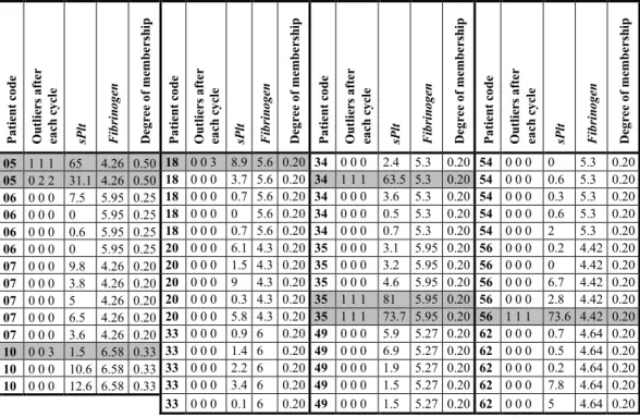
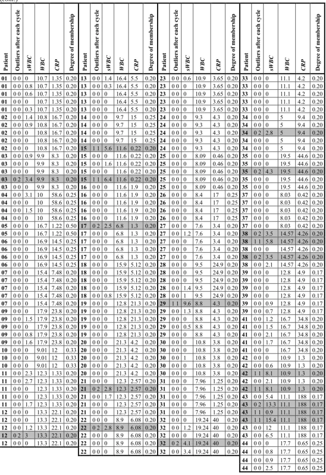
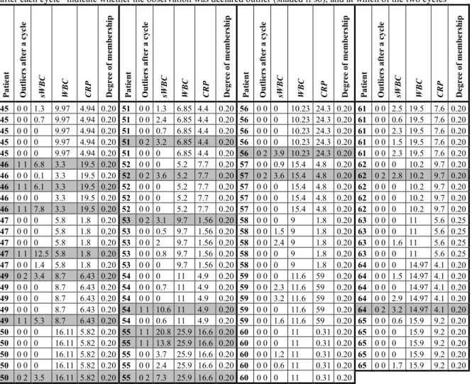
Many works recognize the necessity to operate with fuzzy data samples in statistical (and regression) analysis, with varying interpretations of the degree of membership, caused by the measurement or interpretation process (see Gao and Gao in [30]). Practical reasons may cause fuzzy samples to emerge. Viertl in [70] discusses that sometimes the membership of a given observation to a given subpopulation is defined using a given classificator (probabilistic, metric, neural network, or subjective). Then the confidence in the correctness of the result of the classificator for a given observation may be interpreted as a degree of membership to the sample of the subpopulation. In medical analysis, a given parameter may be measured in t spatial points (e.g. measurements of different parts of a thrombus) for a given patient. Then the degree of membership to the sample for such measurements may be accepted as 1/t so that to provide equal weight for each patient. Other examples are also reported, such as the case described by Nikolova et al. in [36], where objects are assigned to several groups with a given degree of membership based on how similar they were to the descriptors of those groups, utilizing techniques of Denoeux [21] to interpret fuzzy data in experiments with uncertain outcomes.
As the variables in a regression analysis are assumed correlated, if there is a variable represented by a fuzzy sample entering the regression analysis, its degree of membership applies to the overall multi-dimensional observation of 1
2 3 4 5 6 7 8 9 10 11 12 13 14 15 16 17 18 19 20 21 22 23 24 25 26 27 28 29 30 31 32 33 34 35 36 37 38 39 40 41 42 43 44 45 46 47 48 49 50 51 52 53 54 55 56 57 58 59 60 61 62
regression variables. Once fuzzy data is present, we need to utilize fuzzy regression analysis to explore dependencies between variables (see Section 1 for further discussion on fuzzy regression analysis). A valuable study on fuzzy regression analysis is by Chachi and Taheri in [8], who summarized three classes of approaches to fuzziness in regression analysis.
The first class is the possibilistic class that stems from the works of Tanaka [65, 66], where the fuzzy regression problem is formulated as a mathematical programming problem. Tanaka’s approaches and their sensitivity to outliers was discussed in [58], which lead to development of new algorithms of outlier detection for fuzzy regression models as for example the ones offered in [71]. The methods in this group investigate and develop ways to minimize the spread of the fuzzy parameters under certain constraints. The works [51, 52] developed fuzzy linear regression models linked to varying risk relations to minimize the difference between observed and estimates spreads of the output, relying on the concepts of necessity and possibility. The possibilistic regression modelling was reviewed in detail in [6]. The second class comprises least squares and least absolute methods, which aim to estimate the parameters of the model based on a distance on the space of fuzzy numbers. Some of the main works in this class are of D’Urso [14], who proposed regression models for crisp/fuzzy input-output data, and D’Urso et al. [16] that proposed robust fuzzy linear regression model using least median squares-WLS estimation procedure to deal with data that contains outliers. The work of Dehghan et al. [20] may also be attributed to this group as it uses LS and least absolute deviations methods to compare classical and fuzzy regressions using numerical examples of geographical data with symmetric fuzzy observations. Another notable work of Coppi et al. [13] proposed an iterative procedure with LS estimations for a regression mode to study the connection between crisp inputs and fuzzy output observations. D’Urso and Massari [17] explored the iterative WLS domain over a general linear regression model that includes a general class of fuzzy response variables on a set of crisp or LR2 fuzzy explanatory variables. Bargiela et al. explored iterative techniques to study the coefficients of multiple regressions with fuzzy variables in [2]. DUrso et al. [19] also adopt an exploratory approach to find the best fit of a fuzzy linear regression using a new coefficient of determination and the Mallows index. For the case of imprecise responses, Ferrano et al. [28]
proposed ways to construct linear regression models with accompanying hypothesis testing procedures. The third class is a heuristic class and it collects hybrid approaches to construct fuzzy regression models. Such are the works of Kao and Chyu [36, 37], who employed crisp coefficients and fuzzy error terms in a two-stage LS based procedure for fuzzy regression analysis. Lu and Wang [44] developed and improved fuzzy linear regression models that can avoid the spreads increasing problem, while Chachi et al. [7] demonstrated various practical applications of hybrid fuzzy regression models.
The third class may also be expanded with the discussions on how to expand clusterwise regressions (see the works of Jajuga [34] and Yank and Ko [74] that introduced and developed the concept) in the fuzzy domain. The work [64]
discussed this by combining fuzzy clustering and ridge regressions so that to deal with multicollinearity. The works [18, 25] developed a model for fuzzy linear regression utilizing fuzzy clusterwise linear regression that combined symmetrical crisp predictor and fuzzy response variables.
Another similar classification of fuzzy regression methods was also proposed by Jinn et al [35], who outlined a class of approaches utilizing Tanaka’s ideas, and another class that combines the fuzzy least square approaches, pioneered by Diamond [22]. The review work of Chukhrova and Johannssen [10] relied on almost 500 sources to encapsulate thoroughly the various trends, approaches and applications of fuzzy regression analysis. The work identified the major and minor fields of fuzzy regression analysis, and then explored possibilistic approaches as well as fuzzy least square approaches. It also stressed the application of machine learning techniques in fuzzy regression analysis. The work also outlined several minor fields such as fuzzy probabilistic approaches, fuzzy clusterwise regressions, simulation techniques in fuzzy regressions, etc. One of the research questions in [10] was also to investigate the areas of reported practical implementations of fuzzy regression analysis. While engineering and environmental research prevail as implementation areas, the second largest group is that of business administration and economics. Case studies in that respect range from workforce forecasting [43] to project evaluations [33], analysis of macroeconomic parameters [58; 42], analysis of gross domenstic product [75], and stock price forecasting [38].
Other works discuss the impact of outliers in fuzzy regression models. As argued by Gao and Gao [30], sometimes outliers or influence points enter the data set for regression due to various unavoidable causes. This impedes the practical implications and adequacy of the fuzzy regression methods. Therefore, they investigated outlier detection procedures for fuzzy regressions using type-2 trapezoidal fuzzy numbers. Jinn et al. [35] elaborated on the importance of influential observations (that includes outliers) in regression analysis, highlighting the hidden flaws from the fitting process affecting the quality of the regression model. They further developed procedures for fuzzy regressions using the Cook distance, but only adapted those to the general fuzzy regression model, while in other cases their procedures only ended in a simple rejection of outliers with no subsequent analysis. Kwong et al. [41] also discuss the inherited fuzziness of experimental data and show an application of fuzzy regression in manufacturing processes, accounting for outlier rejection for the model accuracy through Peter’s fuzzy regression. The works of Chan et al [9] and Gladysz and Kuchta [31] also demonstrate the necessity to reject outliers for fuzzy regression analysis in real-world applications from engineering and manufacturing. The proposal introduced by Nasrabadi et al. [54] discusses ways to apply linear programming and fuzzy least squares to the outlier detection in fuzzy regression analysis. The importance of outlier detection was also raised by Mashinchi et al. [48], where the authors developed two stage LS approach with no user defined variables. The first stage detects outliers, while the second stage uses the purged sample to fit a regression model with the model fitting measure minimized with a hybrid optimization technique. Yet, this two-stage procedure did not assume that some of the outliers 1
2 3 4 5 6 7 8 9 10 11 12 13 14 15 16 17 18 19 20 21 22 23 24 25 26 27 28 29 30 31 32 33 34 35 36 37 38 39 40 41 42 43 44 45 46 47 48 49 50 51 52 53 54 55 56 57 58 59 60 61 62
may return to the data set as the model develops. All those works show that regression modelling over fuzzy data is highly applicable to many data analysis problems, and the proper rejection of outliers in those procedures are of paramount importance for the adequacy and validity of the constructed models in practice.
When fuzzy data is present, our setup is similar to what we presented in Section 2. Yet, the ith observation
(
x yi i; mes)
ofthe sample now belongs to the Population with a degree of membership µ ∈i [0 1), . We can organize the degrees of membership of all the observations in an n-dimensional membership vector
(
1 2)
T, , , n
µ= µ µ µ
.
A suitable method to identify the coefficients of (3) is the WLS method (see [73]). It aims to derive the estimate βˆWLS ,cur of the coefficients such that to minimize the weighted sum of square differences between the measured and the estimated response values, as follows:
{ }
2( )
n1( )
2 n1( )
2 n1 2WLS mes T mes
i i i i i i i i
ˆ ˆ i ˆ i ˆ i
ˆ arg min ˆ arg min y x ˆ arg min y ˆy arg min uˆ
β β β β
β χ β µ β µ µ
= = =
= = − = − =
∑
∑
∑
(5)
Such a setup imposes several difficulties that we need to address, namely:
• how to identify and reject the outliers in the sample;
• how to find the following parameters based on the purged sample:
o the estimates βˆ=
(
β βˆ ˆ1, 2,,...,βˆq)
T of the unknown coefficients, their confidence intervals and covariance matrix;o the estimate σˆu of the standard deviation of the unexplained error and its confidence interval;
o the pvalue of the hypotheses for nullity of βˆj for j=1, 2,…, q and the pvalue of the hypotheses for adequacy of the model;
o the adjusted coefficient of multiple determination Radj2 , which shows what part of the initial variance of Y is explained by the model, considering the count of determined parameters.
4. LEAST SQUARE SOLUTION OF THE LINEAR REGRESSION PROBLEM WITH KNOWN OUTLIERS OVER FUZZY DATA
Let us first construct a linear model, based on part of the observations (the non-outliers, the others being treated as outliers). If flag variable fi for the ith observation equals to 1, then that ith observation
(
x yi i; mes)
is included in the model, whereas if fi equals to 0 then that ith observation(
x yi i; mes)
is considered an outlier. The flag variables could be organized in an n-dimensional data flag vector(
1 2)
Tf= f , f , , fn
. All initially available observations can be denoted as the quadruplet
(
ymes; ;X µ; f)
. In fact, the model is constructed on1 cur n
in i
n i f
=
=
∑
observations, which shall be referred to as in-observations. The absolute numbers of the in-observations can be organized in nincur-dimensional vector(
1 2 incur)
cur cur cur cur T
a a, , a, , , a,n
δ = δ δ δ
. The count of the outliers is ncurout = −n nincur (which form the set of out-observations) and their absolute numbers can be organized in an noutcur-dimensional vector:
(
1 2 curout)
cur cur cur cur T
b b, , b, , , b,n
δ = δ δ δ
. We can solve the optimization task (4) using singular value decomposition (SVD) [60]. The procedure is realized in Algorithm 1 below, based on the quadruplet
(
ymes; ;X µ; f)
.ALGORITHM 1:CONSTRUCTION OF THE LINEAR REGRESSION MODEL WITH KNOWN OUTLIERS
STEP A. Separate the initial observations in
(
ymes; ;X µ; f)
into outliers and in-observations (non-outliers) according to the values of fbased on the following steps:
A1. Set: i=1, ia=1, and ib=1.
A2. If fi =1 then set δa,iacur=i, and ia=ia+1.
A3. If fi = 0 then set δb,ibcur=i, and ib=ib+1.
1 2 3 4 5 6 7 8 9 10 11 12 13 14 15 16 17 18 19 20 21 22 23 24 25 26 27 28 29 30 31 32 33 34 35 36 37 38 39 40 41 42 43 44 45 46 47 48 49 50 51 52 53 54 55 56 57 58 59 60 61 62
A4. Set i=i+1.
A5. If i≤n then go to A2.
A6. Set: nincur =ia−1, and noutcur =ib−1. A7. Set:
(
1 2 incur)
cur cur cur cur T
a a, , a, , , a,n
δ = δ δ δ
, and
(
1 2 outcur)
cur cur cur cur T
b b, , b, , , b,n
δ = δ δ δ
.
A8. Define the current nincur×q dimensional design matrix Xcur, whose rows are all
µ
i ixT for which fi=1:cur cur
a,i a,i
i ixcur δ xδ µ = µ
, for i=1, 2, …, nincur.
A9. Define the current nincur-dimensional vector of response values ymes,cur, whose elements are all
µ
i iymes, for which fi=1: a,icur a,icurmes,cur mes
yi = µδ yδ , for i=1, 2, …, nincur.
A10. Define the current noutcur×q dimensional outlier matrix Xoutcur, whose rows are all
µ
i ixT for which fi=0:cur cur
b,i b,i i out,ixcur δ xδ µ = µ
, for i=1, 2, …, ncurout.
A11. Define the current noutcur-dimensional outlier vector of response values ymes,cur, whose elements are all
i iymes
µ
, for which fi=1: b,icur b,icurmes,cur mes
out ,i
y = µδ yδ , for i=1, 2, …, noutcur.
STEP B. The Xcur could be factored to the product of three matrices using the SVD decomposition:
cur T
X =W S V× × (6)
Here, W is an nincur×q dimensional column-orthonormal matrix with columns wj (for j=1, 2, …, q); S is an q x q dimensional diagonal matrix with non-negative elements sj (for j=1, 2, …, q) on the main diagonal, called singular values;
V is a q x q dimensional orthonormal matrix with columns vj (for j=1, 2, …, q).
STEP C. The SVD decomposition (6) is usually executed by a computer program and is subject to round-off errors. We need to define which singular values are in fact small positive real values and which are in fact zeros (but estimated as small positive real values due to round-off errors). Therefore we correct the singular values sj to scorj (as per [57, 67]) in four steps:
C1. If sj is non-positive, then scorj =0.
C2. If sj is positive, then we compute an estimate of the unit vector wj as wnonzeroj =X v / scurj j . C3. If the angle between wj and wnonzeroj
is less or equal to 1 deg, and the length of wnonzeroj
is within [0.99; 1.01], then scorj =sj.
C4. If the angle between wj and wnonzeroj
is greater than 1 deg or if the length of wnonzeroj
sits outside of the interval [0.99; 1.01], then scorj =0.
STEP D. According to [60] we can solve (4) using the current coefficient vector
10 corj
T mes,cur
q j
WLS ,cur
cor j
i j
s
ˆ w y v
β s
=
>
=
∑
STEP E. We can calculate consecutively the following parameters that relate to outlier rejection:
E1. The current vector of estimated response values ˆycur =XcurβˆWLS ,cur. E2. The current vector of the WLS residuals uˆcur =ymes,cur−ˆycur. E3. The current residual sum of squares:
( )
21 nin
cur cur
i ˆi
RSS u
=
=
∑
.E4. The current estimate of the standard deviation of the unexplained error: σˆucur = RSScur
(
nincur−q)
.E5. The current q q× dimensional covariance matrix of the parameters:
( )
2 1 110 corj
cur cur q T cor cur
u j i i j i, j i q, j q
s
K σˆ v v / s k
≤ ≤ ≤ ≤
=
>
=
∑
= .1 2 3 4 5 6 7 8 9 10 11 12 13 14 15 16 17 18 19 20 21 22 23 24 25 26 27 28 29 30 31 32 33 34 35 36 37 38 39 40 41 42 43 44 45 46 47 48 49 50 51 52 53 54 55 56 57 58 59 60 61 62
E6. The current standard errors of the parameters: σˆβcurj = kcurj, j for j=1, 2, …, q.
E7. The current (1-
α
)-confidence intervals for each of the parameters1 1
2 curin j 2 incur j
LS ,cur cur LS ,cur cur
j ˆj t α;n qˆβ ,ˆj t α;n qˆβ
β β σ β σ
− − − −
∈ − +
for j=1, 2, …, q. Here,
1 2;nincur q
t−α − is the
(
1−α /2)
quantile of the t-distribution with nincur−q degrees of freedom [32].
E8. The current p-values of the hypotheses for nullity of βˆj: j 2 incur
(
j)
cur cur cur
value, t ,n q j ˆ
p β = ×CDF − −β /σβ , for j=1, 2, …, q. Here, CDFt,nincur−q
( )
. is the cumulative distribution function of the t-distribution with nincur−q degrees of freedom (see [32]).E9. The current (1-
α
)-confidence intervals of the standard deviation of the unexplained error:1 2 incur 2 incur
cur cur cur cur
in u in u
ucur
,n q ,n q
ˆ ˆ
n q n q
,
α α
σ σ
σ χ χ
− − −
− −
∈
. Here, cur
,nin q
χ
γ − is the γ -quantile of the χ2-distribution with nincur−q degrees of freedom (see [32]).E10. The current total sum of squares:
2
1 1
cur cur
in in
n n
cur mes,cur mes,cur cur
i i in
i i
TSS y y / n
= =
=
∑
−∑
.E11. The current adjusted coefficient of multiple determination:
( )
( )
2 1
1
incur
adj,cur cur
in
n RSS
R n q TSS
= − −
− .
E12. The current ANOVA test pvalue for overall adequacy of the model:
( ) ( )
( )
1 1
cur 1
in
incur
value,adcur F,q ,n q
n q TSS RSS
p CDF
q RSS
− −
− −
= − −
. Here, CDFF,q ,n−1 incur−q
( )
. is the cumulative distribution function of the F-distribution with q-1 and nincur−q degrees of freedom (see [32]).STEP F. To test if any of the in-observations is an outlier, we need to calculate the externally Studentized residuals. The pvalue for the hypothesis H0 that a particular observation is not an outlier can be calculated since given H0 its externally Studentized residual follows a t-distribution with nincur− −q 1 degrees of freedom. The required pvalue may be found using ideas from [53] by calculating consecutively:
F1. The current nincur×nincur dimensional hat matrix of the parameters:
( ) ( )
2 1 cur1 curin in
cur cur cur cur T cur cur
u i, j i n , j n
H X K X / σˆ h
≤ ≤ ≤ ≤
= = .
F2. The current predicted residuals: ˆripred ,cur =uˆicur/
(
1−hi,icur)
, for i=1, 2, …, nincur. F3. The current estimate of the standard deviation of the predicted residuals:( ( )
2) (
1) (
1)
1
icur
pred ,cur cur cur cur
in i,i
i cur
i,i
ˆs RSS ˆu / n q / h
h
= − − − − −
, for i=1, 2, …, nincur. F4. The externally Studentized residuals: ˆtipred ,cur =ˆripred ,cur/ sˆipred ,cur, for i=1, 2, …, nincur.
F5. The current pvalue of the hypotheses that the observations
(
xicur;yimes,cur)
are not outliers:( )
2 cur 1
in
pred ,cur
value,in,icur t ,n q ˆi
p = ×CDF − − −t , for i=1, 2, …, nincur. Here, CDFt,nincur− −q 1
( )
. is the cumulative distribution function of the t-distribution with nincur− −q 1 degrees of freedom (see [53]).STEP G. To confirm that the outliers (i.e. the data points, where fi equals to 0) are indeed outliers, we need to calculate their Studentized residuals. We can calculate the pvalue for H0: “A particular observation initially declared outlier is not an outlier”, since, given H0 its Studentized residual follows a t-distribution with nincur−q degrees of freedom. The count of observations declared outliers is noutcur = −n nincur. If noutcur>0, we can find the pvalue by calculating consecutively [53]:
G1. The current estimated predicted response values: ˆyout ,icur =xout ,iT βˆLS ,cur, for i=1, 2, …, noutcur. 1
2 3 4 5 6 7 8 9 10 11 12 13 14 15 16 17 18 19 20 21 22 23 24 25 26 27 28 29 30 31 32 33 34 35 36 37 38 39 40 41 42 43 44 45 46 47 48 49 50 51 52 53 54 55 56 57 58 59 60 61 62
G2. The current estimate of the standard deviation of the predicted response values:
( )
2pred ,cur cur T cur
u out ,i out ,i
out ,i
ˆs = σˆ +x K x , for i=1, 2, …, noutcur.
G3. The current pvalue for the hypothesis H0 that observations
(
xout ,i out,icur ;ymes,cur)
are not outliers:2 cur
in
cur mes,cur
out,i out,i
value,out,icur t,n q pred ,cur
out,i
ˆy y
p CDF
− ˆs
−
= × − , for i=1, 2, …, noutcur. Here, CDFt,nincur−q
( )
. is the cumulative distribution function of the t-distribution with nincur−q degrees of freedom (see [32]).Algorithm 1 allows to reject outliers from the initial sample (in step F), but also in step G it tests to confirm the outlier status of those data points identified as such in Step F. This makes Algorithm 1 flexible and allows it to contribute to the proper quality and quantity of data for fuzzy regression analysis. The model is constructed only on the predefined set of in-observations (i.e. non-outliers). Importantly, Algorithm 1 gives as an output the pvalue of a hypothesis test for outliers of each measurement in the dataset. We use different approaches to calculate the pvalue for the in-observations (i.e. the data points, where fi=1) and for the outliers (i.e. the data points, where fi=0). This algorithm will later become a working engine in a large procedure that works on varying outliers (see Section 5).
The rationale of steps C1-C4 comes from the basic property of SVD decomposition X vcurj =s wj j
(see [67]). If the singular value is positive, then both sides of the equation could be divided to sj, and wnonzeroj
would be almost a perfect estimate of wj
. If the singular value is zero, then the basic property of the SVD decomposition degenerates to equality of two null vectors (X vcurj = =0 0 wj
). Then obviously the wnonzeroj
would be an estimate of a null vector divided by zero, hence it should be quite different from wj
.
5. LEAST SQUARE SOLUTION OF THE LINEAR REGRESSION PROBLEM WITH UNKNOWN OUTLIERS OVER FUZZY DATA
In Section 4 we offered a procedure that constructed a regression model by finding the coefficients (5) using the WLS method. However, this algorithm did not change the status of the data points, i.e. the initial separation to in-observations and out-observations (outliers) remained unchanged. In this section, we shall develop another approach that relies and uses Algorithm 1, yet its task is to assess the outliers and to find the characteristics of the model for different samples iteratively in several cycles. The main reason to use cycles is that as a rule the outliers appear in the initial sample due to some sort of errors in the measurement process (e.g. equipment failure, human error, etc.). As those errors are of miscellaneous nature, the outliers may have varying order of magnitude. Those outliers with higher order can then hide (mask) the ones of smaller order making the latter look as legitimate in-observations in the outliers detection procedure.
Therefore, in each cycle we remove only the outliers with the highest order of deviation from the data sample. Initial results from this approach for the case of crisp data samples is reported by Tenekedjiev and Radoinova in [68].
Assume that the maximum count of cycles permitted is Cmax. The first cycle would start by declaring all data points as in- observations. Alternatively, we can think that the 0th cycle has identified no outliers in the data set. The cth cycle would then start by constructing a model using the in-observations after the (c–1)th cycle. We will calculate the adjusted coefficient of multiple determination for this model. All the outliers can be purged with independent statistical tests for each of the in-observations. The purged observations are added to those declared outliers from the (c–1)th cycle. Then an intermediate model is constructed, based on the current in-observations. At the end of the cth cycle, outliers are only those observations, where the null hypothesis was rejected. All the other observations are added back to the in-observations after the cth cycle.
We can perform the Benjamini-Hochberg step-up multiple testing procedure controlling the false discovery rate (FDR) for independent test statistics to confirm the status of each observation declared outlier (see [4, 5] for discussion of the method). The FDR should be less or equal to a predetermined FDRmax (see also [3] for discussion on FDR). Unlike the p- value in the single testing procedure, which measures the number of false rejections out of all cases where H0 was true, the FDR measures the number of false rejections out of all rejections of H0. The procedures that utilize FDR deal with the expected proportion of false discoveries and were elaborated as an alternative to extremely demanding controlling procedures in multiple testing, such as the Bonferroni correction (for discussion on the Bonferroni approach see [49, 50, 61]). The following considerations justify the deployment of FDR-based multiple testing procedure:
a) The outliers rarely exceed 20% of the data points;
b) If a small amount (e.g 10%) of the declared outliers are in fact legitimate, then the in-observation set will change insignificantly (e.g. from 80% to 78%, i.e. 80% – 10% ×20%=78%);
1 2 3 4 5 6 7 8 9 10 11 12 13 14 15 16 17 18 19 20 21 22 23 24 25 26 27 28 29 30 31 32 33 34 35 36 37 38 39 40 41 42 43 44 45 46 47 48 49 50 51 52 53 54 55 56 57 58 59 60 61 62