Convergence stories of post- socialist Central- Eastern European countries

The Manchester School. 2021;00:1–20. wileyonlinelibrary.com/journal/manc

|

O R I G I N A L A R T I C L E

Convergence stories of post- socialist Central- Eastern European countries

Dániel Baksa

| István Kónya

This is an open access article under the terms of the Creative Commons Attribution- NonCommercial- NoDerivs License, which permits use and distribution in any medium, provided the original work is properly cited, the use is non- commercial and no modifications or adaptations are made.

© 2021 The Authors. The Manchester School published by The University of Manchester and John Wiley & Sons Ltd.

1Institute for Capacity Development, International Monetary Fund, Washington, DC, USA

2Institute of Economics, Center for Economic and Regional Studies, Budapest, Hungary

3Faculty of Economics and Business, University of Pécs, Pécs, Hungary

4Department of Economics, Corvinus University, Budapest, Hungary Correspondence

István Kónya, Center for Economic and Regional Studies, Budapest, Hungary.

Email: konya9@gmail.com Funding information

Higher Education Institutional Excellence Program 2020 of the Ministry of Innovation and Technology, Grant/Award Number: TKP2020- IKA- 02; Hungarian Scientific Research Fund, Grant/Award Number: K116033

Abstract

This paper views the growth and convergence process of five Central- Eastern European economies between 1996 and 2019— the Czech Republic, Hungary, Poland, Slovenia and Slovakia— through the lens of an open economy, stochastic neoclassical growth model with simple financial frictions.

Our main question is whether shocks to the growth rate of productivity (‘trend’) or shocks to the external interest pre- mium are more important to understand the volatility of GDP growth and its components. We find that while GDP growth fluctuations can be traced back to productivity shocks, the composition of GDP— and consumption in particular— was driven particularly by premium shocks. Investment- specific and labor market shocks are also important. Our panel estima- tion allows us to separate global and local components for the productivity- trend and interest premium shocks. Results indi- cate that the global trend component is well approximated by the growth rate of the advanced European Union economies, and we also find tentative evidence that recent investment be- havior is driven to a large extent by European Union funds.

K E Y W O R D S

Bayesian estimation, interest premium, small open economy, stochastic growth, technology shocks

J E L C L A S S I F I C A T I O N E13; O11; O41; O47

1 | INTRODUCTION

Our goal in this paper is to examine the growth and convergence process of five Central and Eastern European member states of the European Union (the Czech Republic, Hungary, Poland, Slovenia and Slovakia— henceforth, CEE) through the lens of the stochastic neoclassical growth model, for the period 1996– 2019. In this we follow Aguiar and Gopinath (2007) and García- Cicco et al. (2010), who estimate similar models for Latin American countries (Mexico and Argentina). We believe that the five CEE countries are a good laboratory for the neoclassical model for the following reasons: (a) they are emerging economies that are highly open both to international trade and external finance, (b) their performance is broadly in line with the predictions of the neoclassical model, where convergence is driven by improvements in total factor productivity (TFP) and capital accumulation, (c) openness al- lows countries to finance some of their additional investment and consumption from abroad, which is exactly what happened in the CEE countries after transition in the 1990s and (d) Also, after the intro- duction of market reforms in the early 1990s, the CEE economies have reasonably similar institutions to the advanced market economies of Western Europe, the natural reference group.

The literature has identified two main shocks that drive stochastic growth in small, open economies like the CEE countries. Aguiar and Gopinath (2007) compare Mexico and Canada, and conclude that in the former shocks to trend productivity growth are more important than in the latter. The main rea- son is that in emerging economies, such as Mexico, the trade balance is counter- cyclical. Transitory TFP shocks imply a pro- cyclical trade balance, since households want to save part of the temporary windfall gains. Permanent and lasting trend shocks, in contrast, imply improving growth performance for a while, leading to increases in current and future permanent income. In that case, households want to consume some of the future gains now, which implies a trade deficit.

García- Cicco et al. (2010) note that Aguiar and Gopinath (2007) ignore the role of financial fric- tions and shocks. In particular, they argue that external financing conditions— which can be taken as exogenous for small, open emerging countries— are important growth determinants. They estimate a financial frictions augmented RBC model on a century of Argentine data, and conclude that includ- ing interest premium shocks in the estimation greatly reduces the importance of trend productivity shocks. Increases in interest premia induce recessions and improve the trade balance at the same time;

thus, they can also explain the counter- cyclicality of the latter. Moreover, in the absence of financial frictions the trade balance is a random walk, which is at odds with the data in emerging economies.

That said, García- Cicco et al. (2010) find that growth volatility is mainly due to transitory technology shocks, at least in Argentina and Mexico.

Other papers have also followed up on the technology versus interest premium debate. Naoussi and Tripier (2013) and Guerron- Quintana (2013) showed that a common trend productivity compo- nent better explains the medium- term GDP growth volatility in African countries than the financial shocks. In contrast, Tastan (2013) finds that, in Turkey, financial shocks are more important. Many papers investigate the role of financial intermediation. Zhao (2013) builds a model where agents face liquidity constraints, and it is changes in liquidity that lead to fluctuations in the risk premium. Minetti and Peng (2013) assumes asymmetric information between domestic and foreign creditors, which be- comes effective when income prospects worsen. This leads to a large response in external financing, which increases the country risk and the effective foreign interest rate.

We contribute to this literature in a number of ways. First, we reevaluate the findings of Aguiar and Gopinath (2007) and García- Cicco et al. (2010) in the context of the CEE countries. We find that while interest premium shocks are important for understanding GDP components, persistent shocks to productivity are the most critical contributors to the volatility of GDP growth. In other words, pro- ductivity has a strong random walk component, and even transitory technology shocks are estimated

to be very persistent. The latter result also casts doubt on whether transitory technology shocks can be separately identified, especially once we include hours in the estimation and allow for labor market disturbances. To paraphrase Aguiar and Gopinath (2007), in our countries the trend is the financial frictions augmented cycle.

Second, and perhaps most interestingly, we estimate the exogenous driving forces of economic growth in a panel. While the time series are short, using a panel of four countries gives us degrees of freedom to identify the underlying shock processes. Using a panel we can separate ‘global’ shocks that affect all countries from ‘local’ shocks that are specific to a country. We show that the global com- ponents of both the trend productivity shock and the interest premium shock have a useful economic interpretation. In particular, the global trend component co- moves very strongly with the growth rate of the ‘old’ European Union countries (EU 15). The implicit common interest rate component also tracks the EU 15 average real interest rate until 2008, but diverges from it sharply afterwards. This finding is consistent with a narrative of the financial crisis in which wedges opened up both between the financial markets of advanced and emerging countries, and between benchmark interest rates and corporate/household lending rates. Our results also relate to Aizenman et al. (2018), who find that the role of global factors in the level and volatility of economic growth increases after the financial crisis in emerging economies.

We make a number of additional methodological contributions, mostly related to the model setup.

We include external consumption habits, which is an alternative to the estimated very persistent pref- erence shock used by García- Cicco et al. (2010). We use adjustment costs to investment instead of capital, and we add an investment- specific shock. This specification was shown to capture the invest- ment dynamics better in a business cycle setting (Christiano et al., 2005). When we plot our estimated investment- specific shock, we find an interesting co- movement between the shock and the magnitude of European Union funds flowing into the CEE countries. This suggests that in addition to the growth and financial environments, external funds were a major determinant of investment dynamics.

We use a labor market specification that is growth consistent and does not require the inclusion of an ad- hoc trend in the value of leisure. As we later explain, this necessitates adding a working capital channel and using a gross output production function to get reasonable predictions for interest pre- mium shocks. In addition to the technical reasons, we also think that the working capital channel is an important propagation mechanism of changes in financial conditions. With this modification the risk premium or capital outflow shock generates a contractionary effect on GDP and thereby the estima- tion is able to separate the supply and financial shocks. The working capital channel was included in other papers as an amplification mechanism for emerging markets (Neumeyer & Perri, 2005). Finally, we use total labor hours as an observable, and we add a labor supply shock to the estimation. On the one hand, observing hours should make the identification of technology shocks more precise. On the other hand, changes in labor market regulation and taxes were important in the CEE countries.

Our model is deliberately simple. We want to focus on a few key mechanisms that influence the medium- term growth, so we omit other channels such as sticky prices and explicit monetary policy.

We do, however, estimate a simple form of wage rigidity, which the data strongly reject. Also, note that while we work with a modified version of the García- Cicco et al. (2010) model, the trade balance remains counter- cyclical in response to the risk premium shock and to the trend productivity shock.

The paper proceeds as follows. In Section 2, we present the basic stylized facts of growth in the CEE countries in the 1996– 2019 period. In Section 3, we describe the stochastic growth model. In Section 4, we estimate the stochastic version of the model, present results from a variance decompo- sition exercise and evaluate the potential role of wage rigidity. Using the estimation results, Section 5 presents interesting findings that we believe strongly validate our estimation results. Finally, Section 6 concludes and discusses future avenues for research.

2 | THE MODEL

We use a modified version of the stochastic, neoclassical growth model described in García- Cicco et al. (2010), or GPU henceforth. Ours is a one- sector, small open economy, where output is used for household consumption, capital investment, net exports and government consumption. Production requires labor and capital. Final good and factor markets are competitive, with flexible prices. The engine of growth is exogenous improvements in productivity; we specify the productivity process later. For simplicity, and given the demographics of the Visegrad countries, we assume that there is no population growth.

It is well known that aggregate variables are more persistent than the basic neoclassical model predicts, even at the annual frequency (Christiano et al., 2005). In our case, this is an important issue, since the estimation starts at an arbitrary initial condition, determined by data availability (typically 1995). As we discussed in the previous section, the behavior of consumption and investment is heavily influenced by the exact timing of economic transition in each country. For this reason, we add a few real rigidities to the basic model which capture the slow adjustment of the main macro variables. We, therefore, assume external habits in consumption and adjustment costs to investment.

An important deviation from GPU is that while they assume GHH preferences (Greenwood et al., 1988), we opt for a more standard separable specification (King et al., 1988; henceforth KPR).

The reason for this is that GHH preferences have a counterfactual prediction for labor hours in catch- ing- up economies. As we show below, our preference specification does not suffer from this issue, but a drawback is that interest premium shocks become expansionary (they are contractionary under GHH preferences).

Therefore, we assume a working capital channel, which was shown to provide useful amplification for financial shocks (Mendoza, 2010). We work with a gross output production function, and impose financing requirements on intermediate inputs as well as the wage bill. Overall, we are able to con- struct a production structure that leads to plausible predictions both along the medium- run transition path and along the short- run business cycle.¹ In particular, working capital on gross output is a suffi- ciently strong cost channel that the interest premium shock again becomes contractionary.

2.1 | Households

The representative household solves the following problem:

where C_t is consumption, h_t is hours worked, D_t+1 is foreign debt carried into the next period, R_t is the gross interest rate on debt and Ξ_t is lump- sum taxes that finance government spending.² Households earn

1Another paper that employs the working capital channel to explain stylized labor market facts in emerging economies is Altug and Kabaca (2017).

𝔼₀

∞

∑

t=0

𝛽^t [

log(

C_t−𝜒C_t−1)

−𝜃_th^𝜔_t 𝜔

]

s. t. C_t+D_t=W_th_t+D_t+1

R_t + Π_t− Ξ_t,

2We assume that government consumption is purely wasteful. Equivalently, we could include it in the utility function in an additively separable form.

wages (W) and profits (Π) from the representative firm that they own. Note that consumption is subject to external habit formation (C_t−1).

There are three structural shocks that affect household decisions. First, we take taxes (government spending) to be exogenous and random:

Second, the interest rate on foreign bonds is subject to exogenous disturbances. The interest rate also has an endogenous component, which depends on the external indebtedness of the economy (Schmitt- Grohé & Uribe, 2003):

where

Finally, labor supply— or more broadly, the labor market— is influenced by an exogenous term 𝜃_t , given as:

The first- order conditions of the problem are given as follows:

where Λ_t is the Lagrange multiplier associated with the budget constraint. The final condition is the bud- get constraint, which was presented above.

2.2 | ^Firms

Factor, intermediate and final good markets are perfectly competitive. We start with the specification of gross output for the representative firm:

where K_t is capital input and M_t is the amount of intermediate inputs. The variable X_t represents the sto- chastic trend component of productivity, which evolves according to the following process:

logΞ_t=( 1−𝜌_𝜉)

logΞ +𝜌_𝜉logΞ_t−1+𝜈^𝜉_t.

R_t=R+𝜓(

e^Dt∕Yt−dy−1)

+e^𝜖r,t−1,

𝜖_r,t=𝜌_r𝜖_r,t−1+𝜈_r,t.

log𝜃_t=( 1−𝜌_h)

log𝜃+𝜌_hlog𝜃_t−1+𝜈^h_t

1

C_t−𝜒C_t−1= Λ_t 𝜃_th^𝜂_t= Λ_tW_t Λ_t=𝛽R_t𝔼tΛ_t+1,

(1) Y^G_t =

[

Υe^atK^𝛼_t (

X_th_t)1−𝛼]1−𝜇

M^𝜇_t,

X_t X_t−1=g_t logg_t=(

1−𝜌_g)

logg+𝜌_glogg_t−1+𝜈^g_t.

In addition, we include a transitory productivity shock a_t, as in Aguiar and Gopinath (2007) and García- Cicco et al. (2010). Note that ϒ is a constant which is included so that we can choose units conveniently (see below).

Firm profits are give as follows:

where I_t stands for gross investment, and

Note that we impose a working capital financing requirement on the wage bill and on interme- diate inputs, so that the firm has to pre- finance these fully. We also add a shock to gross investment (𝜖̃_i,t ). The purpose of this shock is to drive a wedge between the Euler equations of consumption and investment.

We derive the first- order conditions in two steps. First, we optimize out the use of intermediate inputs, which leads to

Plugging this back into the gross output production function, we can express the total production in terms of value added:

where Y_t=e^atK^𝛼_t (

X_th_t)1−𝛼

. Combining this expression with (4) and substituting it into (2), we can re- write profits as

where the second equality follows from a convenient normalization, Υ (1−𝜇)𝜇

𝜇 1−𝜇 =1.

The second step in solving the representative firm's problem is to find the labor demand and capital investment. Using the derivation above, we can state the problem in value added form as follows:

(2) Π_t=

[ ΥK^𝛼_t (

X_th_t)1−𝛼]1−𝜇

M^𝜇_t −R_tM_t−R_tW_th_t−I_t,

(3) K_t+1= (1−𝛿)K_t+

[ 1−𝜙

2 (e^̃𝜖i,tI_t

I_t−1 −g )2]

I_t.

(4) R_tM_t=𝜇Y^G_t

Y^G_t = (𝜇

R_t )₁₋^𝜇

𝜇

ΥY_t,

Π_t= (1−𝜇)Y^G_t −R_tW_th_t−I_t

= (1−𝜇) (𝜇

R_t ) ^𝜇

1−𝜇

ΥY_t−R_tW_th_t−I_t

=R

𝜇 𝜇−1

t Y_t−R_tW_th_t−I_t,

maxΠ₀=𝔼0

∞

∑

t=0

𝛽^tΛ_t Λ₀

[ R

𝜇 𝜇−1

t K^𝛼_t(Xth_t)^1−𝛼−R_tW_th_t−I_t ]

s. t. K_t+1= (1−𝛿)K_t+ [

1−𝜙 2

(I_te^̃𝜖i,t I_t−1 −g

)2] I_t,

where the stochastic discount factor reflects that households are the ultimate owners of firms. Using q_t for the usual Tobin's q multiplier for the capital accumulation constraint, the first- order conditions are given by the following equations:

3 | SHOCK ESTIMATION

In order to estimate the stochastic shocks, we log- linearize the equilibrium conditions around the de- terministic steady state. The observables are the growth rates of GDP, consumption, investment and hours and the trade balance– GDP ratio. To the greatest extent possible, we use raw data. Thus, we only demean the growth rates (except for hours, which are stationary both in the model and in the data) with the country- specific average growth rates of GDP per capita. This is the simplest way to remove the additional growth that comes from economic transition.

Notably, we do not use observed interest rates in the baseline estimation. This is standard in RBC- type models, and the main reason is that the real interest rate that is relevant for household and firm decisions might differ substantially from real interest rates calculated from policy or money market rates. In fact, one of our goals is to compare our implicit, model- based interest rate to an observed time series. As we show in Section 5, this turns out be a quite illuminating exercise.

The main challenge for the estimation is that we have a relatively short time series, namely, annual observations between 1996 and 2019. While using quarterly data are possible, the advantage of higher frequency comes with the cost of additional noise. Since our purpose is to learn about the growth process and slow- moving shocks, we think the annual frequency is more suitable for our purposes. To capture quarterly dynamics reasonably well, additional nominal and real rigidities are needed, which would make the model much more complicated. An important assumption behind our exercise is that these frictions are less important for annual data, and can be captured without explicitly modeling monetary policy and exchange rates.

We gain degrees of freedom through two main strategies. First, we estimate the model on a panel of five Central- and Eastern European (CEE) countries. These economies share a largely common economic history, and they are all transitioning from central planning to market economies. They all joined the European Union in 2004, and have been converging to the ‘old’ member states for most of the sample period. We assume that the structural parameters and the shock autoregressive parameters are common across the five countries, but we allow for country- specific shock innovations (see the details below). These assumptions are routinely made in reduced form panel studies that use country- level data. In fact, our specification is more flexible, since we allow for time- varying ‘fixed effects’ in the form of the country- specific shock innovations.³

R

1 1−𝜇

t W_th_t= (1−𝛼)Y_t q_t=𝛽𝔼t

[ R

𝜇 𝜇−1

t+1

𝛼Y_t+1

K_t+1 + (1−𝛿)q_t+1 ]Λ_t+1

Λ_t 1=q_t

[ 1−𝜙

2 (I_te^𝜖̃i,t

I_t−1 −g )2

e^̃𝜖i,t−𝜙 (I_te^𝜖̃i,t

I_t−1 −g )I_te^𝜖̃i,t

I_t−1 ]

+𝛽𝔼tq_t+1𝜙

(I_t+1e^𝜖̃i,t+1 I_t −g

) (I_t+1e^𝜖̃i,t+1 I_t

)2

Λ_t+1 Λ_t .

3We also tried adding the Baltic countries to our sample, but the results were much more noisy. We suspect this is because the three Baltic economies have much less in common with our CEE countries. They are all much smaller, they were part of the Soviet Union, and they have much stronger economic links with Scandinavia than the CEE countries, whose main economic partner is Germany.

Second, in our baseline specification, we calibrate most of the model parameters, and focus on the shock processes. The static parameters are easy to set using steady- state conditions. There are three dynamic parameters where this is not possible: the debt sensitivity of the interest rate (𝜓), the investment adjustment cost (𝜙) and the strength of consumption habit (χ). It is well known that DSGE models suffer from serious identification problems (Canova & Sala, 2009). When we tried to esti- mate all three parameters, the MH chains were not converging, so we have little trust in the results.

Experimentation reveals that, at most, one dynamic parameter can be estimated reliably. Given our interest in risk premium shocks, we chose to estimate the debt elasticity parameter, and set the other two to standard values from the literature. Results for other specifications are available upon request:

the main conclusions remain robust.

Turning to the shock processes, we assume that trend productivity shock and interest premium shock innovations contain both common and country- specific components:

where j indexes countries. The innovations 𝜈_g and 𝜈_r represent the external growth and financial environ- ments, which are likely to be important determinants of growth in the CEE countries. All other shocks are assumed only to have local innovations.⁴ As discussed above, we impose the same autoregressive param- eter for the five countries for each shock. This is partly because these economies have a similar structure, and also because when estimating country- specific AR(1) terms, we cannot reject the hypothesis that they are the same across economies. This might be the consequence of the short time series, which is an exter- nal constraint we cannot do much about. Even with the common AR term, we believe that our specifica- tion gives us enough flexibility to uncover common and country- specific drivers of the main macro series in question.

Returning to the structural parameters, we follow standard practice and use equations in the deter- ministic steady state to calibrate as many parameters as possible. We set the discount factor to 𝛽=0.98 , and the long- run growth rate to g=1.0237, where the latter is the average per capita value for the EU 15 countries in the sample period. The long- run average interest rate is given as the ratio of the two values. We set the steady- state investment– GDP ratio to the sample average for each country using the chain- linked volumes for investment and GDP.⁵ Assuming a depreciation rate of 𝛿=0.05, we can then compute the adjusted capital– output ratio k∕ (gy). This yields the capital share parameter 𝛼, which we allow to be country- specific, and long- run GDP per hours.

The other expenditure items are set as follows. We impose a uniform government spending share of Ξ∕Y=0.1, which is in line with the data for the CEE countries. Since the long- run debt level is exogenous in the model, and average data from a short sample can be very misleading for these values, we simply set d∕y=0 for all three countries. This means that the long- run trade balance is also zero.

(5) logg^j_t=𝜌_glogg^j_t−1+𝜈_g,t+𝜈^j_g,t

(6) 𝜖^j_r,t=𝜌_rlog𝜖^j_r,t−1+𝜈_r,t+𝜈^j_r,t,

4Note that in the log- linear representation of the model, we rescale the investment shock to ^𝜖i,t= −𝜙g²(1−𝛽𝜌) ̃𝜖_i,t. This also implies that a positive innovation to ^𝜖i,t is associated with a decrease in the cost of investment, that is, the shock is

expansionary.

5An alternative is to use the nominal ratio, which is better from a statistical point of view. In the CEE countries, however, the relative price of investment declined significantly over the sample period. This means that investment expenditure in nominal terms does not adequately reflect the time series of the physical units of capital being created.

Plugging the investment share, the trade balance and the share of government spending into the GDP identity then yields the steady- state consumption– output ratio.

Recall that we use a gross output production function. Thus, we also need to calibrate the share of intermediate inputs (𝜇). We use data from Eurostat on gross output and value added. Our measure of intermediate share is simply given by

where Y and Y^G are observations of value added and gross output for the total economy at current prices.

We normalize the average level of hours to h=0.3, which is a standard value in the literature. This is without loss of generality, and the only role of this normalization is to pin down the parameter 𝜃, as can be seen from the last steady- state condition. We need a value for the inverse of the Frisch elasticity of labor supply, where we follow García- Cicco et al. (2010) and use 𝜔=1.6. This leads to an elasticity of 1∕0.6, which is in line with the parameterization of RBC models that rely on an elastic labor supply to deliver volatilities for GDP and its components in line with the data.

For the two dynamic parameters discussed above, we set 𝜒=0.5, which is equivalent to a quarterly value of 0.84. This is at the high end of DSGE estimates, but, given our annual frequency, significantly lower values would mean habits are unimportant. For the investment adjustment cost parameter, we use 𝜙=2. This is in line with Smets and Wouters (2003), whose mean estimate for the Euro Area is around 7 in a quarterly setting.

Table 1 summarizes the calibrated parameters. Most of them are common across countries, except for the capital share, the share of intermediates and the value of leisure. We now turn to the estimation of the shock processes.

3.1 | Estimation results

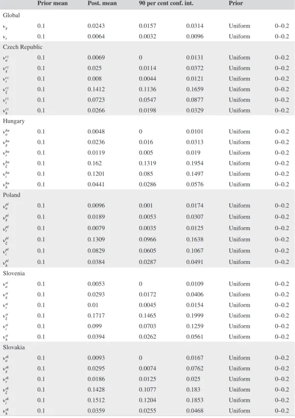
The model is estimated using Bayesian techniques (An & Schorfheide, 2007). We impose flat (uni- form) priors on all shock persistences on the [0, 0.99] interval, and assume that these parameters are the same across the five countries. We allow, however, for country- specific innovations as described in the previous section. We use flat priors for all the standard deviations of the— global or local—

innovations, with a range of [0, 0.2]. Finally, we impose a (somewhat) informative prior for the only structural parameter that we estimate (𝜓).

Data includes chain- linked annual growth rates for GDP, gross fixed capital formation and actual individual consumption for the CEE countries, downloaded from Eurostat. The trade balance is mea- sured by the ratio of net exports to GDP at current prices (source: Eurostat). We use the growth rate of total hours to measure labor input, also downloaded from Eurostat. The sample period is 1996– 2019 for all countries.

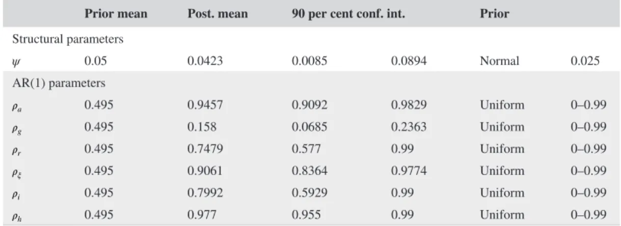
Tables 2 and 3 contain the prior distributions and the estimation results. The shock processes are fairly precisely estimated. Except for the trend shock, the shocks are quite persistent, but clearly iden- tified within the bounds. It is noteworthy to emphasize that although our sample period is short and we use flat priors, the data are informative about the parameter values.

Notice that the data has a hard time disentangling the two technology shock components, namely, the transitory shock a_t and the trend shock g_t. The former is extremely persistent, while the latter is not. This suggests that productivity growth in the CEE countries might be a random walk, Christiano et al. (2010) has found the same for U.S. productivity. Indeed, when we omit the transitory technology

𝜇=1− 1 T

T

∑

t=1

Y_t Y^G_t ,

shock from the estimation entirely, the main results are almost identical. To preserve comparability with Aguiar and Gopinath (2007) and García- Cicco et al. (2010), we present results with the technol- ogy shock included.

3.2 | Variance decomposition

Our main exercise is to decompose the growth rates of GDP, the demand side components and the trade- balance to GDP ratio into contributions of various shock innovations. We have seven items:

global trend (𝜈_g), local trend (𝜈^j_g), global premium (𝜈_r), local premium (𝜈^j_r), technology level (𝜈^j_a), gov- ernment (𝜈^j_gov), investment (𝜈^j_i) and labor (𝜈^j_h) shocks. The variance decomposition shows the relative importance of the estimated structural shocks. Table 4 presents the results of the exercise where we simulate the model using the estimated shock persistences and standard deviations.

TABLE 1 Calibrated parameters

Parameters Value

Common

Discount factor β 0.98

Long- run growth g 1.0124

Depreciation rate δ 0.05

Consumption habit χ 0.5

Investment cost ϕ 2

Frisch elasticity ω 1.6

Steady- state debt/GDP dy 0

Country- specific

CZ HU PL SI SK

Capital share α 0.375 0.302 0.253 0.324 0.332

Share of intermediates μ 0.602 0.574 0.555 0.544 0.598

Value of leisure θ 12.36 12.85 13.13 12.82 12.61

TABLE 2 Bayesian estimation priors and results: Structural and AR(1) parameters Prior mean Post. mean 90 per cent conf. int. Prior Structural parameters

ψ 0.05 0.0423 0.0085 0.0894 Normal 0.025

AR(1) parameters

𝜌_a 0.495 0.9457 0.9092 0.9829 Uniform 0– 0.99

𝜌_g 0.495 0.158 0.0685 0.2363 Uniform 0– 0.99

𝜌_r 0.495 0.7479 0.577 0.99 Uniform 0– 0.99

𝜌_𝜉 0.495 0.9061 0.8364 0.9774 Uniform 0– 0.99

𝜌_i 0.495 0.7992 0.5929 0.99 Uniform 0– 0.99

𝜌_h 0.495 0.977 0.955 0.99 Uniform 0– 0.99

Note: For uniform priors, the prior range is presented. For the normal prior, the standard deviation is shown.

TABLE 3 Bayesian estimation priors and results: Standard deviations

Prior mean Post. mean 90 per cent conf. int. Prior Global

𝜈_g 0.1 0.0243 0.0157 0.0314 Uniform 0– 0.2

𝜈_r 0.1 0.0064 0.0032 0.0096 Uniform 0– 0.2

Czech Republic

𝜈^cz_a 0.1 0.0069 0 0.0131 Uniform 0– 0.2

𝜈^cz_g 0.1 0.025 0.0114 0.0372 Uniform 0– 0.2

𝜈^cz_r 0.1 0.008 0.0044 0.0121 Uniform 0– 0.2

𝜈^cz_𝜉 0.1 0.1412 0.1136 0.1659 Uniform 0– 0.2

𝜈^cz_i 0.1 0.0723 0.0547 0.0877 Uniform 0– 0.2

𝜈^cz_h 0.1 0.0266 0.0198 0.0329 Uniform 0– 0.2

Hungary

𝜈^hu_a 0.1 0.0048 0 0.0101 Uniform 0– 0.2

𝜈^hu_g 0.1 0.0236 0.016 0.0313 Uniform 0– 0.2

𝜈^hu_r 0.1 0.0119 0.005 0.019 Uniform 0– 0.2

𝜈^hu_𝜉 0.1 0.162 0.1319 0.1954 Uniform 0– 0.2

𝜈^hu_i 0.1 0.1201 0.085 0.1497 Uniform 0– 0.2

𝜈^hu_h 0.1 0.0441 0.0286 0.0576 Uniform 0– 0.2

Poland

𝜈^pl_a 0.1 0.0096 0.001 0.0174 Uniform 0– 0.2

𝜈^pl_g 0.1 0.0189 0.0053 0.0307 Uniform 0– 0.2

𝜈^pl_r 0.1 0.0079 0.0035 0.0125 Uniform 0– 0.2

𝜈^pl_𝜉 0.1 0.1309 0.0966 0.1638 Uniform 0– 0.2

𝜈^pl_i 0.1 0.0829 0.0605 0.1067 Uniform 0– 0.2

𝜈^pl_h 0.1 0.0384 0.0287 0.0491 Uniform 0– 0.2

Slovenia

𝜈^si_a 0.1 0.0053 0 0.0109 Uniform 0– 0.2

𝜈^si_g 0.1 0.0293 0.0172 0.0406 Uniform 0– 0.2

𝜈^si_r 0.1 0.01 0.0045 0.0154 Uniform 0– 0.2

𝜈^si_𝜉 0.1 0.1717 0.1465 0.1999 Uniform 0– 0.2

𝜈^si_i 0.1 0.099 0.0703 0.1259 Uniform 0– 0.2

𝜈^si_h 0.1 0.0394 0.0262 0.0561 Uniform 0– 0.2

Slovakia

𝜈^sk_a 0.1 0.0093 0 0.0167 Uniform 0– 0.2

𝜈^sk_g 0.1 0.0295 0.0074 0.0762 Uniform 0– 0.2

𝜈^sk_r 0.1 0.0186 0.0125 0.025 Uniform 0– 0.2

𝜈^sk_𝜉 0.1 0.1428 0.1077 0.183 Uniform 0– 0.2

𝜈^sk_i 0.1 0.1512 0.1204 0.1853 Uniform 0– 0.2

𝜈^sk_h 0.1 0.0359 0.0255 0.0468 Uniform 0– 0.2

Global and local growth shocks explain 46– 65 per cent of the volatility of GDP growth, while transitory technology shocks are not very important. Moreover, we estimate the transitory shock to be very persistent, which makes it difficult to disentangle from ‘true’ growth shocks. Therefore, the distinct role of productivity shocks is consistent with the idea that, during the pre- crisis period, growth expectations played a major role in the CEE economies. Changes in the external growth environment and in income expectations seem to have been the main drivers of aggregate GDP growth. Labor supply shocks were also important, especially in Hungary and Poland. Poland implemented its labor market reform in the middle of the 2000s. After the financial crisis, Hungarian interventions (e.g. the governments since 2009 decreased the income taxes and gradually cut back the social transfers) made the labor market more flexible and thus had a positive effect on Hungarian GDP growth.

Consumption and investment are also functions of productivity growth, but the picture is more heterogeneous and other factors like premium shocks and investment shocks have a larger impact.

Premium shocks influence the composition of aggregate demand, and they are also partly behind the volatility of the trade- balance, and its effect on total GDP growth is limited. The Hungarian econ- omy was fueled by cheap credit before the crisis, and it had to go through a significant balance sheet TABLE 4 Variance decomposition

𝝂_g 𝝂_r 𝝂^j_a 𝝂^j_g 𝝂^j_r 𝝂^j

𝝃 𝝂^j

i 𝝂^j

h

GDP growth

CZ 31.57 0.66 8.49 33.53 1.04 4.09 4.74 15.88

HU 24.34 0.52 2.64 23.07 1.82 4.38 8.1 35.13

PL 28.97 0.75 11.59 17.54 1.16 3.56 3.72 32.71

SI 23.38 0.64 3.28 34.11 1.58 4.66 6.2 26.14

SK 21.07 0.41 9.31 31.08 3.52 2.87 11.94 19.79

Consumption growth

CZ 22.7 12.07 2.9 24.11 19.08 4.33 6.03 8.78

HU 17.99 7.75 0.91 17.05 26.98 3.19 7.36 18.77

PL 26.65 10.06 4.85 16.14 15.63 2.45 3.32 20.91

SI 18.14 8.17 1.22 26.47 20.09 4.09 6.58 15.24

SK 11.3 5.33 2.31 16.66 45.64 1.78 9.16 7.81

Investment growth

CZ 12.35 7.29 1.4 13.12 11.53 0.88 51.2 2.23

HU 6.19 2.88 0.31 5.86 10.04 0.37 70.83 3.52

PL 11.47 4.55 2.18 6.95 7.07 0.32 62.13 5.33

SI 8.04 3.37 0.48 11.73 8.3 0.51 64.22 3.35

SK 3.8 2.08 0.76 5.6 17.79 0.23 68.37 1.37

Trade balance to GDP

CZ 1.46 23.33 1.39 1.55 36.88 3.37 29.84 2.19

HU 0.7 12.39 0.38 0.66 43.11 2.28 36.41 4.07

PL 1.18 23.19 2.95 0.72 36.03 2.69 26.65 6.58

SI 0.99 15.72 0.58 1.44 38.67 3.25 35.56 3.79

SK 0.38 6.6 0.75 0.56 56.49 0.96 32.95 1.31

Note: The table shows the shock variance decomposition of the four key variables based on model simulations. The simulations use the baseline calibration, together with the posterior means of shock persistences and standard errors.

adjustment post- crisis. The local premium shock is also important for Slovakian domestic demand, especially for consumption growth.

In the past decade, investment might also have been strongly affected by the inflow of EU transfers.

It is particularly interesting that investment- specific shocks not only drive investment growth itself, but also the volatility of the trade balance. While the model does not have an explicit role for external funds, the investment- specific shocks can capture at least some of these extra developments. We pro- vide some suggestive evidence in the next section that this is indeed the case.

Overall, our results indicate that both trend productivity shocks and interest premium shocks are important to understand the growth experience of the CEE countries. As in Aguiar and Gopinath (2007), but in contrast to García- Cicco et al. (2010), we find that the volatility of GDP growth is mainly driven by shocks to the trend component of productivity. Nonetheless, interest premium shocks are important for understanding the evolution of the main GDP components, and consumption growth in particular. In addition, labor market shocks and especially investment- specific shocks have played a significant role. Restricting attention to productivity and interest premium shocks might thus be too restrictive, at least in the context of the CEE economies.

3.3 | Robustness

3.3.1 | Real wage rigidity

We experimented with many variations on the baseline estimation strategy, and our main conclusions remain robust. One of these was incorporating real wage rigidity into the mode and estimation. It is unclear whether nominal rigidities are relevant at the annual frequency. If the answer is yes, wage rigidity is the most likely candidate (Blanchard & Galí, 2010; Olivei & Tenreyro, 2010). Fortunately, it is easy to modify our simple framework to accommodate real wage rigidity. In an Online Appendix, we derive a labor market specification with real wage rigidity, based on Erceg et al. (2000).

Empirical evidence for many countries (Babecky et al., 2010) suggest that firms adjust their wages annually. This is equivalent to a quarterly Calvo parameter of about 0.75. At the annual frequency, this translates to a Calvo parameter of about 0.3. We are using quadratic adjustment costs, so we link the parameter 𝜑 to the equivalent Calvo coefficient in the estimation using the formal correspondence between our wage Phillips curve and the identical equation in Erceg et al. (2000). We impose a beta prior on the Calvo equivalent, with a prior mean of 0.2 and standard deviation of 0.1. This fairly wide prior encompasses both the flexible case and the rigid case.

The posterior mean is 0.035, with a tight posterior confidence interval of 0.023– 0.046. The hypoth- esis that real wage rigidity is an important channel at the growth frequency is very strongly rejected by the data. The other parameter estimates are very similar to the baseline case. We, therefore, conclude that while potentially important for some countries and episodes, wage rigidity does not seem to be relevant for the general growth experience of the CEE economies in our sample period.

3.3.2 | Observing the real interest rate

In our model, as a robustness check, we also tried to observe the long- term real interest rate. However, the long- term real interest rate is not necessarily consistent with the logic of the neoclassical model.

In these models, the real interest rate expresses those effective equilibrium yields that are driven by the external financing premium and marginal product of capital. Thus, this unobserved rate contains

price and non- price- related components as well, that is, the non- price- related components are the un- observed credit constraint and all conditions that directly influence the financial intermediaries. We collected the long- term real interest rate⁶ from the AMECO database from 2002, calculated the differ- ence between the country- level rate and Eurozone long- term real interest rate, and compared the long- term real interest rate differentials. In the previous estimation, we calculated the level of the real interest rate by adding together the steady- state level and dynamic components; in this estimation, the observed variable is the deviation from the Eurozone interest rate.⁷

We present detailed results in an Online Appendix. To summarize, most of the estimated parame- ters and standard deviations are very close to the benchmark estimation. The role of global and local trend shocks remain important factors for the GDP and demand growth. The country- level investment- specific shocks still explain most of the country- level investment growth. Once the real interest rate is observed, the role of the risk premium (local and global as well) is more limited, and, instead of the risk premium shock, the transitory technology shock is another contributor to the domestic demand decomposition. If we observe the real interest rate, the overall volatility of the rates and the contri- bution of the estimated risk premium shocks is lower. Hence, in the alternative estimation, the less volatile risk premium shocks are insufficient to explain the distribution of the domestic demands. In this sense, adding the real interest rate to the estimation puts more weight on the ‘trend is the cycle’

and the technology- driven interpretation of the economic fluctuations of the emerging economies.

4 | EXTERNAL MODEL VALIDATION

After presenting the main results, we discuss additional findings that— while interesting in their own right— provide strong external validation for the estimation exercise. We compare the estimated global components of the trend shock and the interest premium shock to an observable (EU) time series. We also study the investment- specific shock innovations and relate them to EU funding after the 2004 period.

4.1 | Trend growth and investment

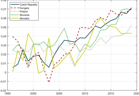
First, we take a closer look at the estimated trend productivity shock. In particular, we want to exam- ine the global component that the estimation uncovered, 𝜈_g,t. Figure 1 plots the global trend innovation against the growth rate of the EU 15 countries.⁸ The rationale for this is that the CEE countries over- whelmingly trade with other EU countries, and the EU 15 represents the ‘core’ economy of the group.

Thus, we expect that external common growth shocks are highly correlated with the growth rate of the EU 15 countries. This is indeed what we find, as Figure 1 shows. The global innovation 𝜈_g,t tracks EU 15 growth very closely, especially since 2004, when the CEE countries joined the European Union.

While only suggestive, this result gives us confidence that the estimation procedure ‘makes sense’.

To further investigate the role of the European Union in the growth process of the CEE countries, we now turn to investment. As we saw above, investment- specific shocks are significant determinants

610Y interest rate minus inflation expectation.

7The underlying tendencies in the observed interest rate differentials are similar to dynamics of the estimated implicit rates.

We are happy to provide further comparison charts upon request.

8These are the ‘old’ EU member states before the expansion of 2004: Austria, Belgium, Denmark, Finland, France, Germany, Greece, Ireland, Italy, Luxembourg, Netherlands, Portugal, Spain, Sweden and United Kingdom.

of the volatilities of investment and the trade balance. For the latter, this is especially true after 2004, when the CEE countries joined the European Union (see the Appendix tables on historical shocks decompositions). A possible explanation for this is the presence of EU structural funds, which have become a significant source of investment spending in the four countries. Overall, net EU payments are on the scale of 2– 5 per cent of gross national income, especially since 2010.

A detailed study of the role of EU funds is beyond the scope of this paper. For a proper understand- ing, we would need to build a model with external transfers and a government sector with its separate investment activity. Instead, we provide some preliminary evidence that EU funds are likely to be an important explanation for the idiosyncratic behavior of investment captured by its specific shock.

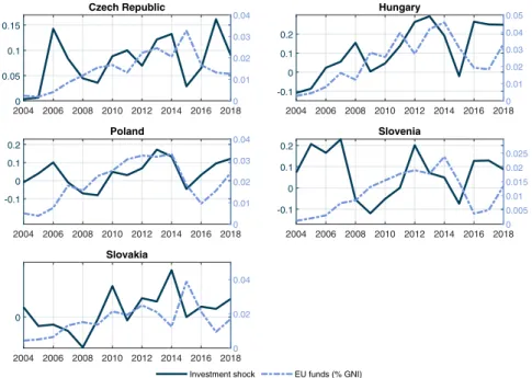
Figure 2 plots the estimated investment shock (𝜖_i,t, left scale) against European Union funds received annually (as a share of GNI, right scale). Data are available from the European Union since 2004, when the CEE countries became members.⁹

Once we adjust for the differences in measurement units, the two time series are fairly similar in our countries. This is particularly the case in Hungary, Poland and Slovakia. While these charts are only suggestive, it is reassuring that the estimation recovers a stochastic shock that can be given a reasonable empirical interpretation.

4.2 | Interest rate and interest premium

In our estimation we do not use observed interest rates; rather, we back them out from the evolution of GDP components. It is interesting to see whether these implicit interest rates ‘make sense’, that is, whether their paths are in line with our prior expectations. We would like to find the following

9http://ec.europa.eu/budge t/figur es/inter activ e/index_en.cfm.

FIGURE 1 Global growth shock component and EU growth. The figure shows the estimated common (‘global’) innovations to trend productivity growth 𝜈_g,t together with the real GDP growth rate of the EU 15 countries

1995 2000 2005 2010 2015 2020

-0.07 -0.06 -0.05 -0.04 -0.03 -0.02 -0.01 0 0.01 0.02 0.03

Estimated global component (%, YoY) EU 15 growth rate (%, YoY)

patterns: high values in the 1990s, a gradual decline before the financial crisis (especially in the 2004–

2008) period, and increased heterogeneity after the crisis. For the latter period, we expect interest rate increases for more heavily indebted countries (Hungary), and decreases for less- indebted countries (the Czech Republic, and to a lesser extent Poland and Slovakia). It is important to note that our implicit interest rates condense price and non- price information that are relevant for intertemporal consumption and investment decisions, and thus can be quite different from the policy rate. This is especially important after the financial crisis, when quantitative restrictions on credit became much more prevalent and low headline interest rates may mask high effective borrowing rates by house- holds and small enterprises.

Figure 3 presents the results. The implicit interest rate have been most stable in the Czech Republic, the richest and most stable economy in the group. Slovenia, the other economic leader until recently, had a deep banking crisis in 2013, which is reflected in the sharp rise in the implicit interest rate afterwards. The two countries that joined the Eurozone by the time of the financial crisis (Slovenia and Slovakia) experienced lower implicit rates in 2009– 2010 than Hungary and the Czech Republic.

Poland, which was the only country to escape recession after 2009, shows the lowest increase in the interest rate after 2009. The experience of Hungary is the most dramatic. In the pre- crisis period, Hungary enjoyed a positive investment climate and became the most heavily indebted economy; sub- sequently, it was most exposed to financial market tightening and balance sheet adjustment. This is reflected in the very low estimated rates until 2007, and the steep rise that started just before the crisis, and continued afterwards. By 2010, Hungarian implicit rates have become the highest in the group, and remained high until 2017.

Recall that similarly to the stochastic productivity trend, we estimated the interest rate innovations with a global and local component. We expect the global component to pick up changes in external financial conditions that effected all CEE countries similarly. As before, we use the EU 15 countries FIGURE 2 EU funding and investment- specific shocks. The figure shows the estimated investment- specific shock (𝜖^j_i,t) for each country (left scale), together with net EU funds received as a share of GNI (right scale)

2004 2006 2008 2010 2012 2014 2016 20180 0.05

0.1 0.15

Czech Republic

0 0.01 0.02 0.03 0.04

2004 2006 2008 2010 2012 2014 2016 2018 -0.1

0 0.1 0.2

Hungary

0 0.01 0.02 0.03 0.04 0.05

2004 2006 2008 2010 2012 2014 2016 2018 -0.1

0 0.1 0.2

Poland

0 0.01 0.02 0.03 0.04

2004 2006 2008 2010 2012 2014 2016 2018 -0.1

0 0.1 0.2

Slovenia

0 0.005 0.01 0.015 0.02 0.025

2004 2006 2008 2010 2012 2014 2016 2018 0

Slovakia

0 0.02 0.04

Investment shock EU funds (% GNI)