GPU accelerated study of a dual-frequency driven single bubble in a 6-dimensional parameter space: the active
cavitation threshold
Ferenc Heged˝usa,∗, K´alm´an Klapcsika, Werner Lauterbornb, Ulrich Parlitzc, Robert Mettinb
aDepartment of Hydrodynamic Systems, Faculty of Mechanical Engineering, Budapest University of Technology and Economics, Budapest, Hungary
bDrittes Physikalisches Institut, Georg-August-Universit¨at G¨ottingen, G¨ottingen, Germany
cResearch Group Biomedical Physics, Max Planck Institute for Dynamics and Self-Organization and Institut f¨ur Dynamik komplexer Systeme, Georg-August-Universit¨at G¨ottingen, G¨ottingen, Germany
Abstract
The active cavitation threshold of a dual-frequency driven single spherical gas bubble is studied numerically. This threshold is defined as the minimum energy required to generate a given relative expansion (Rmax−RE)/RE, where RE is the equilibrium size of the bubble and Rmax is the maximum bubble radius during its oscillation. The model employed is the Keller–Miksis equation that is a second order ordinary differential equation. The parameter space investigated is composed by the pressure amplitudes, excitation frequencies, phase shift between the two harmonic components and by the equilibrium bubble radius (bubble size). Due to the large 6-dimensional parameter space, the number of the parameter combinations investigated is approximately two billion.
Therefore, the high performance of graphics processing units is exploited; our in-house code is written in C++ and CUDA C software environments. The results show that for (Rmax−RE)/RE = 2, the best choice of the frequency pairs depends on the bubble size.
For small bubbles, below 3µm, the best option isto use equal frequencies and low ones in the giant response region. For medium sized bubbles, between 3µm and 6µm, the optimal choice is the mixture of low frequency (giant response) and main resonance frequency. For large bubbles, above 6µm, the main resonance dominates the active cavitation threshold.
Increasing the prescribed relative expansion value to (Rmax−RE)/RE= 3, the optimal choice is always equal frequencies with the lowest values (20 kHz here). Thus, in this case, the giant response always dominates the active cavitation threshold. The phase shift between the harmonic components of the driving has no effect on the threshold.
Keywords: Keller–Miksis equation, bubble dynamics, dual-frequency driving, cavitation threshold, GPU programming
∗Corresponding author
Email addresses: fhegedus@hds.bme.hu(Ferenc Heged˝us),kklapcsik@hds.bme.hu(K´alm´an Klapcsik),werner.lauterborn@phys.uni-goettingen.de (Werner Lauterborn),
ulrich.parlitz@ds.mpg.de (Ulrich Parlitz),robert.mettin@phys.uni-goettingen.de( Robert Mettin)
1. Introduction
1
Sonochemistry is a special branch of chemistry which intends to produce chemical
2
species via the irradiation of a liquid with ultrasound [1–7]. Due to the high ampli-
3
tude pressure waves, bubble clusters are formed in the liquid domain composed of nearly
4
spherical bubbles [8–18]. During their radial pulsation, the high compression ratio might
5
result in thousands of degrees of Kelvin internal temperature inducing chemical reac-
6
tions [19–24]. Some of the interests of sonochemical applications are the production of
7
hydrogen (green fuel) [25–28], free radicals for wastewater treatment [29–32] or nanoal-
8
loys/nanoparticles which are efficient catalysts [33–35].
9
Several experimental results have shown that the application of dual-frequency irra-
10
diation can increase the sonochemical yield significantly (even by 300%) compared to
11
the conventional single frequency case [36–48]. These studies reported that the chemical
12
yield of dual-frequency irradiation is usually higher than the sum of the chemical yields
13
of single frequency sonications. This indicates that there is a synergetic effect between
14
the harmonic components. During the last decades, many theories have been devised to
15
explain this effect: better pattern of the pressure waves inside a sonochemical reactor
16
(e.g. more active zones) [43, 49–51], more cavitation nuclei are generated for feeding
17
the bubble clusters [44, 50–52], increased mass transfer via micromixing [50, 53] or the
18
increased collapse strength of the individual bubbles [39, 41].
19
Still, the theoretical background of the synergetic effect is unclear. Moreover, reports
20
on decreased sonochemical efficiency of dual-frequency irradiation were also published,
21
see e.g. [53]. Many researchers investigated dual-frequency driven single bubbles [54–
22
57] to find evidence for the synergetic effect of this approach and to establish a theory
23
through the investigation of the dynamics of a single spherical bubble. For example,
24
the form of the signal of the external dual-frequency driving (e.g., bigger difference be-
25
tween its minimum and maximum) can produce bubble dynamics having a stronger
26
collapse [26, 58, 59] or a lower active cavitation threshold [60, 61]. The special resonance
27
properties of the bubble caused by dual-frequency excitation (e.g., combination and si-
28
multaneous resonances) can explain the increased cavitational activity [62, 63]. Also, the
29
dual-frequency driving can alter the spherical stability threshold [64] or increase the mass
30
transfer through the bubble interface [65]. The present study focuses on the reduction
31
of the active cavitation threshold, which is usually defined as how much input energy
32
is required (formulated in terms of the pressure amplitudes) to obtain a cavitationally
33
active bubble dynamics. However, in our opinion the results in the literature are not
34
exhaustive enough. The main reason is the large number of parameters involved when
35
using multi-frequency driving. Even in case of a dual-frequency driving, the minimum
36
number of parameters that needs to be investigated is six: two pressure amplitudes,
37
two frequencies, the phase shift between the harmonic components and the bubble size.
38
Therefore, the limited number of investigated parameter combinations in the literature
39
can hide their complex impact on the bubble dynamics.
40
In this sense, the main aim of the present study is to perform high-resolution scans in
41
the 6-dimensional parameter space by exploiting the large processing power of graphics
42
processing units (GPUs). Even with a careful planning of the parameter ranges and their
43
resolution, the total number of parameter combinations is approximately 2 billion, for
44
details see Sec. 3. Such a detailed investigation may help to identify the synergetic effect
45
between the harmonic components of the driving. The employed model is the Keller–
46
Miksis equation that is a second order ordinary differential equation. It is used due to
47
its simplicity as the number of parameter combinations is quite large. The solver used is
48
based on our in-house code written in C++ and CUDA C, and it is free to use under an
49
MIT license. The interested reader is referred to the website [66] of the program package
50
or to its GitHub repository [67]. The software package also has a detailed manual with
51
tutorial examples [68].
52
Beyond the scope of sonochemistry, the results obtained on dual-frequency driven
53
single bubble can have a significant impact on other specialised fields of acoustic cavita-
54
tion. For instance, dual-frequency driving is successfully used in therapeutic applications
55
to decrease the active cavitation threshold [40] and to minimise the damage and mental
56
stress to the patients [69, 70]. In diagnostic ultrasound, it is widely used to enhance
57
the contrast of ultrasound (subharmonic) imaging [71, 72]. Moreover, the dual-frequency
58
technique has importance in bubble sizing [73], boosting sonoluminescence [74] or con-
59
trolling chaotic oscillations of bubbles [75].
60
2. The bubble model
61
The governing equation is the Keller–Miksis equation describing the evolution of the
62
radius of a spherical gas bubble placed in a liquid domain and subjected to external
63
excitation [14]. The second-order, ordinary differential equation reads
64
1− R˙ cL
!
RR¨+ 1− R˙ 3cL
!3
2R˙2= 1 + R˙ cL
+ R cL
d dt
!(pL−p∞(t)) ρL
, (1) where R(t) is the time dependent bubble radius;cL= 1497.3 m/s andρL= 997.1 kg/m3
65
are the sound speed and density of the liquid domain, respectively. The pressure far
66
away from the bubble,p∞(t), is composed by static and by periodic components
67
p∞(t) =P∞+PA1sin(ω1t) +PA2sin(ω2t+θ), (2) where P∞ = 1 bar is the ambient pressure. The periodic components have pressure
68
amplitudes PA1 and PA2, angular frequencies ω1 = 2πf1 and ω2 = 2πf2, and a phase
69
shiftθ.
70
The connection between the pressures inside and outside the bubble at its interface
71
is chosenas
72
pG+pV =pL+2σ R + 4µL
R˙
R, (3)
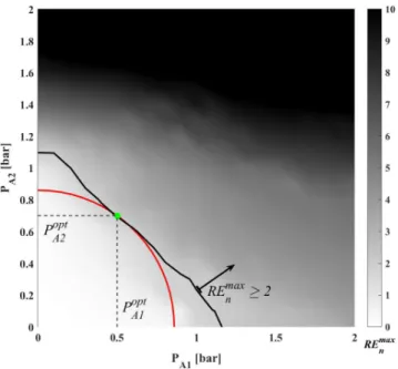
where the total pressure inside the bubble is the sum of the partial pressures of the
73
non-condensable gas, pG, and the vapour, pV = 3166.8 Pa. Thermal effects and mass
74
transfer are not taken into account. The surface tension isσ= 0.072 N/m and the liquid
75
kinematic viscosity isµL = 8.902−4Pa s. The gas inside the bubbleis assumed to obey
76
a simple polytropic relationship
77
pG=
P∞−pV + 2σ RE
RE
R 3γ
, (4)
where the polytropic exponentγfor air is chosen(γ= 1.4, adiabatic behaviour) and the
78
equilibrium bubble radius is RE.
79
System (1)-(4) is transformed into a dimensionless form by the introduction of the following dimensionless variables
τ= ω1
2πt, (5)
y1= R RE
, (6)
y2= ˙R 2π REω1
. (7)
The dimensionless system is written as
˙
y1=y2, (8)
˙
y2= NKM
DKM
, (9)
where the numerator,NKM, and the denominator,DKM, are
NKM= (C0+C1y2) 1
y1
C10
−C2(1 +C9y2)−C3
1 y1 −C4
y2
y1− 1−C9
y2
3 3
2y22−(C5sin(2πτ) +C6sin(2πC11τ+C12)) (1 +C9y2)
−y1(C7cos(2πτ) +C8cos(2πC11τ+C12)), (10) and
80
DKM=y1−C9y1y2+C4C9, (11) respectively.
81
The coefficients are summarised as follows:
C0= 1 ρL
P∞−pV + 2σ RE
2π REω1
2
, (12)
C1=1−3γ ρLcL
P∞−pV + 2σ RE
2π REω1
, (13)
C2=P∞−pV
ρL
2π REω1
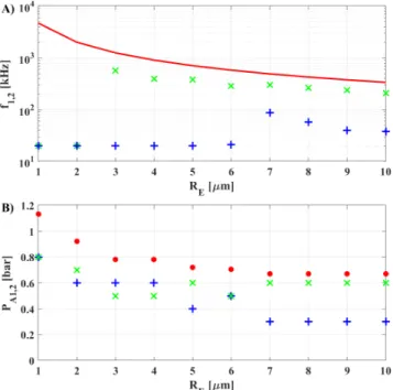
2
, (14)
C3= 2σ ρLRE
2π REω1
2
, (15)
C4= 4µL
ρLR2E 2π ω1
, (16)
C5=PA1
ρL
2π REω1
2
, (17)
C6=PA2
ρL
2π REω1
2
, (18)
C7=RE
ω1PA1
ρLcL
2π REω1
2
, (19)
C8=RE
ω1PA2
ρLcL
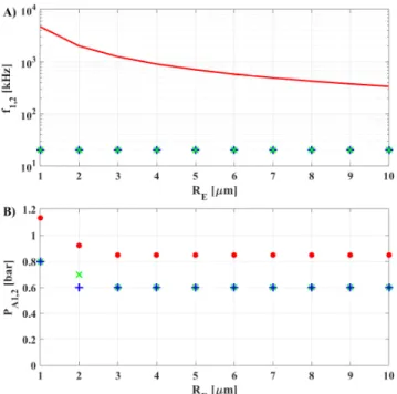
2π REω1
2
, (20)
C9=REω1
2πcL
, (21)
C10= 3γ, (22)
C11=ω2
ω1
, (23)
C12=θ. (24)
3. The investigated parameter space
82
Assuming that the liquid ambient properties (temperature and pressure) and the liq-
83
uid composition are fixed, the main control parameters that affect the bubble dynamics
84
are the properties of the external dual-frequency driving. Therefore, the first five parame-
85
ters investigated here are the pressure amplitudesPA1andPA2, the excitation frequencies
86
f1 and f2 and the phase shift between the harmonic components of the driving θ. In
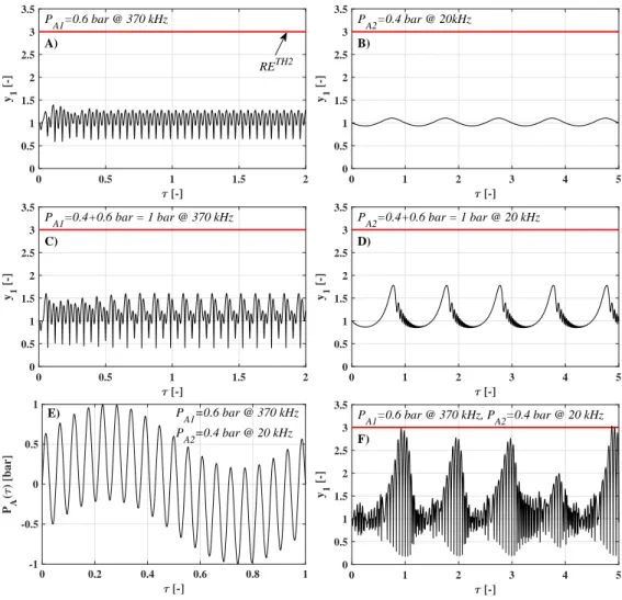
87
addition, the sixth parameter is the equilibrium bubble radiusREcharacterising the size
88
of the bubble since it varies significantly in a sonochemical reactor.
89
The ranges (minimum and maximum values), resolutions and the type of the distri-
90
butions (linear or logarithmic) of the six parameters varied are summarised in Tab. 1.
91
That is, the pressure amplitudes are varied between 0 and 2 bar with an increment of
92
0.1 bar. This means 21 equidistant values of the pressure amplitudes. In order to resolve
93
the different kinds of resonance properties of the system, the resolution of the frequencies
94
(varied between 20 kHz and 2 MHz) is increased to 101. Moreover, a logarithmic scale is
95
applied to resolve the two orders of magnitude difference in the frequency ranges prop-
96
erly. The values of the phase shift are distributed evenly between 0 and 2π(1−1/20)
97
with a resolution of 20 (taking into account the periodicity property). The bubble size is
98
varied between 1 and 10µm with an increment of 0.5µm. This covers the typical ranges
99
of bubble sizes observed during experiments [76–79]. Although the employed parameter
100
resolutions can be considered quite moderate, the total number of parameter combi-
101
nations is approximately 1.89 billion. The overall simulation time was approximately
102
2 weeks using two Nvidia Tesla P100 graphics cards. This justifies the application of
103
high-performance GPU programming mentioned already in Sec. 1.
104
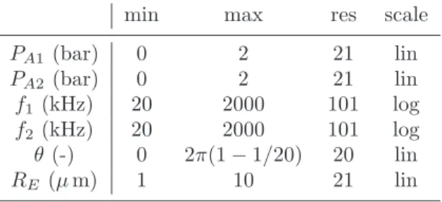
Table 1: Ranges, resolutions and the types of distribution of the control parameters of the 6-dimensional parameter space. The abbreviations lin, log, and res stand for linear, logarithmic, and resolution, respectively.
min max res scale
PA1 (bar) 0 2 21 lin
PA2 (bar) 0 2 21 lin
f1(kHz) 20 2000 101 log
f2(kHz) 20 2000 101 log
θ (-) 0 2π(1−1/20) 20 lin
RE (µm) 1 10 21 lin
4. The numerical procedure
105
The integration procedure is as follows. At each parameter combination, the inte-
106
gration is started from the equilibrium condition y1(0) = 1 and y2(0) = 0. Thus, the
107
co-existence of attractors is not examined as only one initial condition is applied. The
108
first integration phase is stopped at the first local maximum ymax1,1 of the dimensionless
109
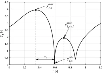
bubble radius y1. The subsequent integration phases are performed from a local maxi-
110
mum y1,nmax to the next local maximumy1,n+1max , see also Fig. 1. The first 512 integration
111
phases are regarded as initial transients and discarded. The properties of the next 64 in-
112
tegration phases are recorded: the local maximaymax1,n , the subsequent minimum bubble
113
radiiy1,nminand the elapsed times betweeny1,nmaxandy1,nmindenoted byτc,n. The dynamics
114
between the local maximum and the subsequent minimum radius is called a collapse
115
phase throughout the paper, even if the pressure amplitudes are so small that the bubble
116
is chemically inactive near the minimum radius. The saved properties of 64 collapses at
117
a single parameter set allow one to perform a statistical analysis as well. Storing data of
118
multiple subsequent collapses are important as a solution can be chaotic, quasiperiodic
119
or periodic with high periodicity. Moreover, many smaller collapses called afterbounces
120
can occur in a single period of the driving after a strong collapse. Thus, recording the
121
property of a single collapse after the transient cannot represent the complex dynamics.
122
This shall be important in the future to investigate the collapse rate (the number of
123
strong collapses in unit time). The present paper focuses only on the strongest recorded
124
collapse at each parameter set.
125
For further investigation, it is important to define a suitable expression to characterise
126
the strength of a collapse. In the literature, many possibilities are available: expansion
127
0 0.2 0.4 0.6 0.8 1 1.2 [-]
0 0.5 1 1.5 2 2.5 3 3.5 4 4.5
y 1 [-]
y1,nmax
y1,n+1 max
y1,nmin
Figure 1: A typical time series of a dimensionless bubble radius y1 show collapses. The characteristic quantities of the first collapse are also presented by the arrows.
ratioRmax/RE=y1max[38, 42, 60, 61, 80], compression ratioRmax/Rmin=y1max/y1min
128
that is related to the maximum temperature of the bubble [42, 81], the quantity of
129
R3max/tc [39, 41, 82] or the relative expansion (Rmax−RE)/RE=y1max−1 commonly
130
used in numerical studies to characterise the magnitude of the oscillation [57, 62, 63].
131
Out of the many possibilities we choose the relative expansion
132
RE=Rmax−RE
RE
=ymax1 −1 (25)
that takes the different values
133
REn =Rmax,n−RE
RE
=y1,nmax−1 (26)
in the course of the oscillation. Our already mentioned numerical investigation, including
134
chemical kinetics, has revealed thatthis quantity has the best correlation with the chemical
135
yield of a bubble [83]. It is widely accepted in the literature that inertial or transient
136
cavitation occurs if the expansion ratio is approximately Rmax/RE =ymax1 > 2; that
137
is, if the relative expansion is RE > 1 [38, 84–86]. In this way, the active cavitation
138
threshold can be givenin terms of the relative expansion denoted by REthr. According
139
to our aforementioned study [83], the chemical yield of a bubble is a smooth, power-
140
like function of the relative expansionRE. Therefore, any given threshold value for the
141
chemical activity must be somewhat arbitrary. The results showed that the chemical
142
activity starts to increase rapidly somewhere betweenRE = 2 and 3. Throughout this
143
paper, these threshold values are investigated in detail denoted byREthr,2andREthr,3,
144
and the synergetic effect of the dual-frequency driving is explained in terms of these
145
thresholds. It must be stressed that the term active cavitation threshold is used as a
146
synonym to the inception of chemical activity in this paper. The detailed discussion of
147
the “classic” terminology of inertial/transient cavitation (and their threshold values) is
148
beyond the scope of the present study.
149
5. Definition of the active cavitation threshold in terms of the pressure am-
150
plitude for dual-frequency driving
151
The definition of the active cavitation threshold in terms of the relative expansion
152
REthr is very powerful as one can estimate the incidence of the chemical activity merely
153
by inspecting the time series of the bubble radius. However, such a threshold can be
154
defined also in terms of the input power I; that is, the minimum power required for
155
chemical activity. In case of a single transducer, the generated pressure amplitudePAis
156
proportional to the square root of the input power: PA ∝√
2IρLcL [39, 80]. Therefore,
157
the active cavitation threshold can be formulated also in terms of the pressure ampli-
158
tudes byPAthr=PAopt, wherePAoptdenotes the minimum pressure amplitude required for
159
chemical activity with single frequency driving. The generalisation for a dual-frequency
160
case can be written as
161
PAthr = q
(PA1opt)2+ (PA2opt)2, (27) taking into account the relationship between the input power and the generated pressure
162
amplitude. Here,PAthr is an equivalent pressure amplitude of a single frequency driving
163
having the same input power as the sum of the input powers of the individual frequency
164
components in the dual-frequency case.
165
To determine a suitable threshold for the pressure amplitude, information about the
166
collapse strength is still necessary. In this sense, PAthr,2 andPAthr,3 mean the minimum
167
(equivalent) pressure amplitudes required to reach REthr,2 and REthr,3, respectively,
168
which are the necessary collapse strengths for chemical activity, see the discussion in
169
Sec. 4. The procedure to determinePA1optandPA2optis demonstrated in Fig. 2 for frequencies
170
f1 = 200 kHz, f2 = 34.76 kHz, phase shift θ = 0 and for bubble size RE = 10µm. In
171
the figure, the colour code is the maximum achievable relative expansionREnmaxplotted
172
as a function of the pressure amplitudes PA1 andPA2. The active cavitation threshold
173
REthr,2 is denoted by the black curve. According to Eq. (27), the pressure amplitude
174
combinations having the same total input power can be represented by circles. The
175
larger the radius of the circle the larger the total input power. The optimal choice
176
of the amplitude pair on the black threshold line corresponds to the circle having the
177
lowest radius (minimal input power). This is demonstrated by the red circle, and the
178
related amplitude pair PA1opt andPA2optis marked by the green dot. In this way, for every
179
combination off1,f2, θandRE, values ofPAthr,2 andPAthr,3 can be associated. Observe
180
that with the help of the active cavitation threshold in terms of the pressure amplitudes,
181
the investigated parameter space is reduced to four dimensions.
182
6. Optimal parameter combination to minimise PAthr,2
183
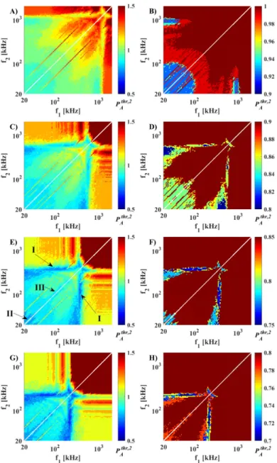
Figure 3 summarises the values of the active cavitation thresholdPAthr,2as a function
184
of the frequencies f1 and f2 between 20 kHz and 2 MHz at different bubble sizes RE.
185
The first, second, third and fourth rows of the subpanels are related to RE = 2µm,
186
4µm, 6µm and 10µm bubble sizes, respectively. The phase shift between the harmonic
187
components of the driving is kept constantθ= 0. Keep in mind that the lower the value
188
ofPAthr,2the lower the required input energy for chemically active cavitation. In the first
189
column of the subpanels, the range ofPAthr,2is kept constant between 0.5 bar and 1.5 bar
190
Figure 2: The determination of the active cavitation threshold in terms of the pressure amplitude for dual-frequency driving.
for a better comparison of the effect of the bubble size RE. In the second column, the
191
ranges are adjusted so that the location of the minima ofPAthr,2can be clearly identified.
192
From the increasing tendency of the adjusted ranges in the second column of Fig. 3, it
193
is clear that the active cavitation thresholdPAthr,2increases with decreasing bubble size.
194
The reason is the higher value of Blake’s critical threshold [87] for smaller bubbles. In
195
addition, three main regions can be identified for local/global minima ofPAthr,2. The first
196
region is related to the main resonance of the system and denoted by I, see Fig. 3E. The
197
main resonance appear as vertical and horizontal stripes in the frequency plane (f1, f2)
198
whose locations are bubble size-dependent according to the linear eigenfrequency of the
199
system [14, 88]:
200
f0= 1 2π
s3γ(P∞−pV)
ρLR2E −2(3γ−1)σ
ρLR3E . (28)
The second region, marked by II in Fig. 3E, is the well-known giant response [14] region
201
located always in the lowest frequency domain. Due to the low frequency, the bubble
202
has enough time to grow large (several times higher than its equilibrium size) resulting
203
in a very strong collapse afterwards. The third region is a local minimum ofPAthr,2 that
204
occurs at the diagonal of the frequency plane (denoted by III). Because of the equal
205
frequencies, this case represents single frequency driven bubbles and thus, it highlights
206
the fact that to produce a certain pressure amplitude, it is more energy-efficient to use
207
two transducers with half amplitudes.
208
For simplicity, the aforementioned regions are marked only in subpanel Fig. 3E. How-
209
ever, all or some of them are present also at other bubble sizes. For small bubbles, case
210
II, the giant response region dominates the frequency plane. In contrast, for large bub-
211
Figure 3: The dual-frequency active cavitation thresholdPAthr,2 (in bar) as a function of the frequencies f1andf2in the range 20 kHz to 2 MHz at different bubble sizesRE. The phase shiftθ= 0 is constant.
The first, second, third and fourth rows of the subpanels are computed atRE= 2µm, 4µm, 6µm and 10µm bubble sizes, respectively.
bles, case I, the main resonance dominates the frequency plane. Between large and small
212
bubbles, there is a somewhat smooth transition from case I to case II or vice versa. Case
213
III never dominates the (f1, f2) plane. It is worth mentioning that case II, the giant
214
response, can be regarded as a sub-region of case III (equal frequencies). However, we
215
keep the distinction to emphasize the application of small frequencies that generates the
216
giant response.
217
Before proceeding further, it is important to discuss the effect of the phase shiftθ. To
218
clearly identify the role ofθ, an animation has been created where the panels similar to the
219
ones shown in the first column of Fig. 3 are presented as a function of all the investigated
220
bubble sizes RE and phase shifts θ. These are changing with time. At fixed bubble
221
sizes, the figures related to different values ofθare almost identical. Therefore, for single
222
spherical bubbles, its effect on the active cavitation threshold can be neglected. The
223
animation is available as supplementary material called EffectOfTheta Animation.avi.
224
The remaining task is to represent the optimal setup of the frequency pairs (minimum
225
PAthr,2) as a function of the bubble size RE. Therefore, for each bubble sizes, the fre-
226
quencies f1andf2are extracted from the location of the global minimum ofPAthr,2. The
227
corresponding pressure amplitudesPA1optandPA2optare also registered to have information
228
about the pressure amplitude distribution between the two frequency components. The
229
results are summarised in Fig. 4. Keep in mind that simulations are carried out with
230
a fine resolution of the bubble size, and Fig. 3 represents only some typical cases. The
231
red line in the top panel of Fig. 4 is the resonance frequency of the bubbles calculated
232
via Eq. (28). The red dots in the bottom panel are the lowest possible values of the
233
active cavitation threshold PAthr,2 at a given bubble size, the corresponding frequencies
234
and amplitudes are marked by the green and blue crosses, respectively (in both panels).
235
Figure 4: The optimal values of the driving frequencies (panel A) and the pressure amplitudes (panel B) for active cavitation thresholdPAthr,2. They are denoted by the blue and green crosses. The red line in panel A) is the size-dependent linear resonance frequency of the bubble. The red dots in panel B) represent the lowest values ofPAthr,2.
The condensed representation of the results in Fig. 4 supports our previous obser-
236
vations. For small bubble radii, approximately below 3µm, the giant response region
237
is the optimal choice with equal frequencies (single frequency driving) and equal pres-
238
sure amplitudes (energy efficiency). For large bubbles, above 6µm, it is important to
239
drive the system nearly at its resonance frequency, see the green crosses in the upper
240
panel. The deviation between the red curve and the green crosses is due to the highly
241
non-linear nature of the bubble dynamics [84, 89–104]. The pressure amplitude of the
242
second frequency component is much smaller (compare the blue crosses in both panels);
243
thus, the main resonance frequency is the dominant component and it plays the major
244
role here. For moderate bubble sizes, between 3µm and 6µm, both the giant response
245
(lowest frequency, here 20 kHz) and the main resonance (close to the red curve in the
246
upper panel) are important for an optimal setup. Observe that the amplitudes are nearly
247
equal in this regime; thus, both frequency components are important. This setup can
248
be observed as a relatively big blue region in Fig. 3D located at the low-high frequency
249
combinations. Since this bubble size region covers the majority of the experimentally
250
observed bubble size distribution [76–79], this finding can be a possible explanation for
251
the synergetic effect of dual-frequency driving using a low-high frequency combination.
252
7. Optimal parameter combination to minimise PAthr,3
253
Although the value of the relative expansionRE= 2 (REthr,2) is an accepted measure
254
for the incidence of chemical activity, some reactions needs much higher collapse strength
255
to have measurable effects (e.g. nitrogen dissociation [19, 105]). Therefore, the evaluation
256
process presented in the previous section (Sec. 6), is repeated forRE= 3 (REthr,3). The
257
corresponding active cavitation threshold in terms of the equivalent pressure amplitude is
258
denoted byPAthr,3. The condensed summary of the results is shown in Fig. 5. The colour
259
code is the same as in case of Fig. 4. The message of the diagram is clear: use small
260
frequencies (giant response) and use equal frequencies with equal amplitudes (energy
261
efficiency). That is, the giant response always dominates the frequency parameter plane
262
regardless of the bubble size. Similarly, as in case ofPAthr,2, the effect of the phase shiftθ
263
is negligible. It is worth mentioning already here that giant response is not a speciality
264
for dual-frequency driving. Therefore, a synergetic effect cannot be recognised in Fig. 5,
265
only energy efficiency. For a detailed discussion see Sec. 8.
266
8. Discussion
267
Dual-frequency driving can be an energy-efficient technique for enhancing the yield in
268
sonochemical applications. The upper bound of the peak value of the pressure amplitude
269
that can be generated is the sum of the amplitudes of the harmonic components
270
PA≤PA1+PA2 (29)
expressing the superposition of the generated pressure waves. Therefore, using two trans-
271
ducers with the same frequencies and amplitudes, and with zero phase difference, one
272
can reduce energy consumption by a factor of two to generate the same amplitude:
273
Figure 5: The optimal values of the driving frequencies (panel A) and the pressure amplitudes (panel B) for active cavitation thresholdPAthr,3. They are denoted by the blue and green crosses. The red line in panel A) is the size-dependent linear resonance frequency of the bubble. The red dots in panel B) represent the lowest values ofPAthr,3.
ISF ∝PA2 IDF ∝PA12 +PA22
= (0.5PA)2+ (0.5PA)2
= 0.25PA2+ 0.25PA2
= 0.5PA2,
(30)
where ISF and IDF are the input powers for the single and dual-frequency driving,
274
respectively. However, this observation cannot be regarded as a synergetic effect, it is
275
purely an energy efficiency consideration of ultrasonic transducers.
276
A real synergetic effect can be observed for active cavitation threshold REthr,2 be-
277
tween bubble sizes 3µm and 6µm, where the application of a low and a high-frequency
278
combination yields the lowest required power to reach the active cavitation threshold.
279
The synergy is the mixture of the giant response (low frequency) and the main resonance
280
(high frequency) phenomena. It is demonstrated through an example in Fig. 6 for a bub-
281
ble size of 5µm. According to Fig. 4, the optimal dual-frequency setup isPA1= 0.6 bar
282
with f1= 370 kHz andPA2= 0.4 bar withf1= 20 kHz. From Fig. 6A-B, it is clear that
283
applying the harmonic components separately, the maximum expansion of the bubble is
284
far from the threshold value REthr,2 (red horizontal line aty1= 3). The dual-frequency
285
signal is presented in Fig. 6E. Observe that how its peak value can be estimated by the
286
addition of the pressure amplitudesPA1and PA2, see also Eq. (29). In Fig. 6C-D, single
287
frequency driven cases are demonstrated employing an increased amplitude ofPA= 1 bar
288
that is the peak value of the dual-frequency signal. In this way, the effect of the appli-
289
cations of two transducers can be simulated using the same frequencies at amplitudes
290
PA1 = 0.6 bar andPA2 = 0.4 bar. The maximum bubble expansions are still far away
291
from the active cavitation threshold. However, with the same pressure amplitudes (same
292
input power) but with a mixture of frequencies, the maximum bubble expansion can
293
be increased significantly, see Fig. 6F. It reaches the active cavitation threshold as it
294
is expected. It must be stressed that such a synergetic effect is hard to find by trial
295
and error due to the high dimensional parameter space. This justifies the application of
296
high-performance GPU computing. Interestingly, many experimental studies reported
297
the synergetic effect of the application of low-high frequency combination using similar
298
frequency combinations, see Refs. [37, 42, 44]. This justifies that the aforementioned
299
phenomenon can be a possible explanation for the synergy.
300
Increasing the active cavitation threshold formREthr,2toREthr,3, the above-described
301
synergetic effect completely disappears. The optimal choice is to use the lowest frequen-
302
cies (20 kHz) for both harmonic components, and use equal amplitudes. This setup
303
represents the energy-efficient exploitation of the giant response phenomenon observed
304
at low-frequency driving. This finding puts to the question of the above demonstrated
305
synergetic effect since the chemical activity increases rapidly with increasing relative ex-
306
pansion RE(the threshold valuesREthr,2/REthr,3 are only estimates for the incidence
307
of the chemical activity). For instance, the production ofOH− radical is approximately
308
4×10⁵, 3×10⁶ and 7×10⁷ molecules during a single collapse for relative expansions
309
RE= 2, 3 and 6, respectively [83]. In this sense, for high chemical yield, the best option
310
is always the generation of giant response without involving and exploiting the main
311
resonance.
312
The study Ref. [83] is carried out with an oxygen bubble placed in water. Even in such
313
a simple configuration, the number of the chemical species is 9 and the number of reaction
314
equations is 44. The different reaction equations are activated at different temperature
315
values; thus, for different collapse strengths, the composition of the chemical products
316
of a bubble can be quite different as well. Therefore, an optimal collapse strength (peak
317
temperature) can exist according to the requirements of the chemical output. This is
318
reported by Yasui et al. [105] with nitrogen bubbles in water, where the production of free
319
radicals decreases with the peak temperature above an optimal value. The reason is that
320
at very high temperature, the nitrogen molecules can dissociate; thus, reaction equations
321
related to nitrogen atoms can play a significant role and consume the free radicals.
322
In conclusion, for every liquid-gas composition, an optimal temperature and collapse
323
strength might be associated depending on the required chemical yield. Therefore, the
324
above-described synergetic effect can be important if the optimal collapse strength in
325
terms of the relative expansion is approximately belowRE= 3.
326
As a final remark, it is very likely that the synergetic effect cannot be explained by
327
a single phenomenon, i.e., by the active cavitation threshold in terms of the pressure
328
amplitude only as it is studied in the present paper. The correct treatment is to take
329
into account the chemical kinetics in the bubble model and compute the production
330
of the required chemical species directly. However, such a computation needs orders
331
of magnitude larger computational resources as the number of the parameters is still
332
0 0.5 1 1.5 2 [-]
0 0.5 1 1.5 2 2.5 3 3.5
y1 [-]
RETH2 PA1=0.6 bar @ 370 kHz
A)
0 1 2 3 4 5
[-]
0 0.5 1 1.5 2 2.5 3 3.5
y 1 [-]
PA2=0.4 bar @ 20kHz B)
0 0.5 1 1.5 2
[-]
0 0.5 1 1.5 2 2.5 3 3.5
y1 [-]
PA1=0.4+0.6 bar = 1 bar @ 370 kHz C)
0 1 2 3 4 5
[-]
0 0.5 1 1.5 2 2.5 3 3.5
y 1 [-]
PA2=0.4+0.6 bar = 1 bar @ 20 kHz D)
0 0.2 0.4 0.6 0.8 1
[-]
-1 -0.5 0 0.5 1
PA() [bar]
E) P
A1=0.6 bar @ 370 kHz PA2=0.4 bar @ 20 kHz
0 1 2 3 4 5
[-]
0 0.5 1 1.5 2 2.5 3 3.5
y 1 [-]
PA1=0.6 bar @ 370 kHz, P
A2=0.4 bar @ 20 kHz F)
Figure 6: Synergetic effect of dual-frequency driving at a bubble size of 5µm. Panel A and C: time series of the bubble radius of single frequency driving with 370 kHz at different pressure amplitudes PA1 = 0.6 bar andPA1 = 1 bar. Panel B and D: time series of the bubble radius of single frequency driving with 20 kHz at different pressure amplitudes PA2 = 0.4 bar andPA2 = 1 bar. Panel E and F:
driving signal and time series of the bubble radius of the dual-frequency driving. The pressure amplitudes arePA1= 0.6 bar andPA2= 0.4 bar with frequenciesf1= 370 kHz andf2= 20 kHz.
high but the complexity of the model increases significantly. In addition, other physical
333
phenomena can also play an important role, for instance, the collapse rate (number of
334
strong collapses in a unit time), spherical stability [91, 106–112] (efficient mixing of the
335
bubble interior with the liquid [24]) or rectified diffusion [113–115] (faster growth of the
336
bubbles to a chemically active state [65]). The study of these effects is in the main focus
337
of our forthcoming papers. Moreover, the dual-frequency driving can have significant
338
influence on the dynamics of a bubble cluster, the size distribution of the bubbles, the
339
nucleation procedure or the structure of the clusters via the secondary Bjerknes forces.
340
These latter effects are already discussed in Sec. 1.
341
9. Summary
342
A dual-frequency driven single spherical bubble was studied numerically. The model
343
employed was the Keller–Miksis oscillator that is a non-linear second-order ordinary
344
differential equation. The main aim was to provide a theoretical background for the
345
synergetic effect of dual-frequency driving in terms of the active cavitation threshold.
346
The investigated parameter space was composed by the pressure amplitudes, frequen-
347
cies, phase shift between the two harmonic components and the bubble size. Even with
348
the moderate resolution of the 6-dimensional parameter space, the total number of the
349
simulated parameter combinations was approximately 2 billion. Therefore, the high pro-
350
cessing power of GPUs was exploited to obtain the results within a reasonable time.
351
The evaluation of the results showed that for an active cavitation threshold (in terms
352
of relative expansion) lower than approximately (Rmax−RE)/RE = 3, the applica-
353
tion of low-frequency driving (giant response) combined with high-frequency component
354
(main resonance) can significantly increase the collapse strength of a bubble; thus, it
355
significantly lowers the required input power to generate chemically active bubbles. This
356
synergetic effect holds for bubble sizes between 3µm and 6µm, which covers the range
357
of the experimentally observed typical bubble size distribution in a bubble cluster. For
358
a higher active cavitation threshold, above (Rmax−RE)/RE = 3, the synergetic effect
359
disappears and the giant response (low frequency) with equal pressure amplitude (energy
360
efficiency) is always the optimal choice. Therefore, the aforementioned synergetic effect
361
plays an important role only if the required collapse strength (induced peak temperature)
362
is moderate for the optimal chemical yield.
363
Acknowledgement
364
This paper was supported by the Alexander von Humboldt Foundation, by the J´anos
365
Bolyai Research Scholarship of the Hungarian Academy of Sciences, by the Deutsche
366
Forschungsgemeinschaft (DFG) grant no. ME 1645/7-1, and by the Higher Education
367
Excellence Program of the Ministry of Human Capacities in the frame of Water science
368
& Disaster Prevention research area of Budapest University of Technology and Economics
369
(BME FIKP-V´IZ).
370
References
371
[1] B. D. Storey, A. J. Szeri, Water vapour, sonoluminescence and sonochemistry, Proc. R. Soc. Lond.
372
A 456 (1999) (2000) 1685–1709.
373
[2] T. J. Mason, Some neglected or rejected paths in sonochemistry – A very personal view, Ultrason.
374
Sonochem. 25 (2015) 89–93.
375
[3] F. Cavalieri, F. Chemat, K. Okitsu, A. Sambandam, K. Yasui, B. Zisu, Handbook of Ultrasonics
376
and Sonochemistry, 1st Edition, 2016.
377
[4] R. J. Wood, J. Lee, M. J. Bussemaker, A parametric review of sonochemistry: Control and
378
augmentation of sonochemical activity in aqueous solutions, Ultrason. Sonochem. 38 (2017) 351–
379
370.
380
[5] K. S. Suslick, N. C. Eddingsaas, D. J. Flannigan, S. D. Hopkins, H. Xu, The chemical history of
381
a bubble, Acc. Chem. Res. 51 (9) (2018) 2169–2178.
382
[6] R. J. Wood, J. Lee, M. J. Bussemaker, Combined effects of flow, surface stabilisation and salt
383
concentration in aqueous solution to control and enhance sonoluminescence, Ultrason. Sonochem.
384
58 (2019) 104683.
385
[7] R. J. Wood, J. Lee, M. J. Bussemaker, Disparities between sonoluminescence, sonochemilumines-
386
cence and dosimetry with frequency variation under flow, Ultrason. Sonochem. 58 (2019) 104645.
387
[8] R. Mettin, S. Luther, C.-D. Ohl, W. Lauterborn, Acoustic cavitation structures and simulations
388
by a particle model, Ultrason. Sonochem. 6 (1) (1999) 25–29.
389
[9] R. Mettin, S. Luther, C.-D. Ohl, W. Lauterborn, Bubble size distribution near a pressure antinode,
390
J. Acoust. Soc. Am. 105 (2) (1999) 1075–1075.
391
[10] W. Lauterborn, C.-D. Ohl, Acoustic Cavitation and Multi Bubble Sonoluminescence, Springer
392
Netherlands, Dordrecht, 1999, pp. 97–104.
393
[11] R. Mettin, Bubble structures in acoustic cavitation, in: Bubble and Particle Dynamics in Acoustic
394
Fields: Modern Trends and Applications, Research Signpost, Trivandrum, Kerala, India, 2005.
395
[12] R. Mettin, From a single bubble to bubble structures in acoustic cavitation, in: Oscillations, Waves
396
and Interactions: Sixty Years Drittes Physikalisches Institut ; a Festschrift, Universit¨atsverlag
397
G¨ottingen, G¨ottingen, Germany, 2007.
398
[13] F. Reuter, R. Mettin, W. Lauterborn, Pressure fields and their effects in membrane cleaning
399
applications, J. Acoust. Soc. Am. 123 (5) (2008) 3047–3047.
400
[14] W. Lauterborn, T. Kurz, Physics of bubble oscillations, Rep. Prog. Phys. 73 (10) (2010) 106501.
401
[15] J. Eisener, A. Lippert, T. Nowak, C. Cair´os, F. Reuter, R. Mettin, Characterization of acoustic
402
streaming beyond 100 MHz, Physics Procedia 70 (2015) 151–154.
403
[16] F. Reuter, S. Lauterborn, R. Mettin, W. Lauterborn, Membrane cleaning with ultrasonically driven
404
bubbles, Ultrason. Sonochem. 37 (2017) 542–560.
405
[17] F. Reuter, S. Lesnik, K. Ayaz-Bustami, G. Brenner, R. Mettin, Bubble size measurements in
406
different acoustic cavitation structures: Filaments, clusters, and the acoustically cavitated jet,
407
Ultrason. Sonochem. 55 (2019) 383–394.
408
[18] D. Fuster, A review of models for bubble clusters in cavitating flows, Flow Turbul. Combust.
409
102 (3) (2019) 497–536.
410
[19] K. Yasui, T. Tuziuti, T. Kozuka, A. Towata, Y. Iida, Relationship between the bubble temperature
411
and main oxidant created inside an air bubble under ultrasound, J. Chem. Phys. 127 (15) (2007)
412
154502.
413
[20] K. Yasui, T. Tuziuti, J. Lee, T. Kozuka, A. Towata, Y. Iida, The range of ambient radius for an
414
active bubble in sonoluminescence and sonochemical reactions, J. Chem. Phys. 128 (18) (2008)
415
184705.
416
[21] D. F. Rivas, L. Stricker, A. G. Zijlstra, H. J. G. E. Gardeniers, D. Lohse, A. Prosperetti, Ultrasound
417
artificially nucleated bubbles and their sonochemical radical production, Ultrason. Sonochem.
418
20 (1) (2013) 510–524.
419
[22] L. Stricker, D. Lohse, Radical production inside an acoustically driven microbubble, Ultrason.
420
Sonochem. 21 (1) (2014) 336–345.
421
[23] S. Merouani, O. Hamdaoui, Y. Rezgui, M. Guemini, Computer simulation of chemical reactions
422
occurring in collapsing acoustical bubble: dependence of free radicals production on operational
423
conditions, Res. Chem. Intermediat. 41 (2) (2015) 881–897.
424
[24] R. Mettin, C. Cair´os, A. Troia, Sonochemistry and bubble dynamics, Ultrason. Sonochem. 25
425
(2015) 24–30.
426
[25] S. Merouani, O. Hamdaoui, Y. Rezgui, M. Guemini, Mechanism of the sonochemical production
427
of hydrogen, Int. J. Hydrog. Energy. 40 (11) (2015) 4056–4064.
428
[26] K. Kerboua, O. Hamdaoui, Sonochemical production of hydrogen: Enhancement by summed
429
harmonics excitation, Chem. Phys. 519 (2019) 27–37.
430
[27] S. S. Rashwan, I. Dincer, A. Mohany, B. G. Pollet, The Sono-Hydro-Gen process (Ultrasound
431
induced hydrogen production): Challenges and opportunities, Int. J. Hydrog. Energy. 44 (29)
432
(2019) 14500–14526.
433
[28] M. H. Islam, O. S. Burheim, B. G. Pollet, Sonochemical and sonoelectrochemical production of
434
hydrogen, Ultrason. Sonochem. 51 (2019) 533–555.
435
[29] P. Riesz, T. Kondo, Free radical formation induced by ultrasound and its biological implications,
436
Free Radical Bio. Med. 13 (3) (1992) 247–270.
437
[30] K. Yasuda, T. Torii, K. Yasui, Y. Iida, T. Tuziuti, M. Nakamura, Y. Asakura, Enhancement of
438
sonochemical reaction of terephthalate ion by superposition of ultrasonic fields of various frequen-
439
cies, Ultrason. Sonochem 14 (6) (2007) 699–704.
440
[31] A. A. Pradhan, P. R. Gogate, Degradation of p-nitrophenol using acoustic cavitation and Fenton
441
chemistry, J. Hazard. Mater. 173 (1) (2010) 517–522.
442
[32] S. Merouani, O. Hamdaoui, Y. Rezgui, M. Guemini, Sensitivity of free radicals production in
443
acoustically driven bubble to the ultrasonic frequency and nature of dissolved gases, Ultrason.
444