Pliant Arithmetics and Pliant Arithmetic Operations

Pliant Arithmetics and Pliant Arithmetic Operations

József Dombi

University of Szeged

Árpád tér 2, H-6720 Szeged, Hungary dombi@inf.u-szeged.hu

Abstract: Fuzzy arithmetic based

α

-cuts, where the result of the

α

-cuts represent an interval. The arithmetic can be understand as an interval arithmetic of the

α

-cuts. Instead of dealing with intervals we are dealing with left and right hand sided soft inequalities which define the interval. We offer a new calculation procedure of arithmetics, when these soft inequalities meet certain properties (i.e. strict monotonously increasing function represent the inequality). We show that the result of linear combinations of linear is also linear and the linear combination of sigmoid is also sigmoid function (i.e. they are closed under linear combination). We give the result of other operation, too. The soft inequalities define an interval by using proper conjunctive and disjunctive operator. We give such operations, too.

Keywords: fuzzy arithmetic, sigmoid function, triangular membership function, membership function, distending function

1 Introduction

The idea the fuzzy quantities could be arithmetically combined according to the laws of fuzzy set theory is due to Zadeh [14]. Soon after, several researchers worked independently along these lines, such as Jain [5], Mizumoto and Tanaka [9, 10], Nahmias [11], Nguyen [12], Dubois and Prade [1]. It was only further on recognized that the mathematics of fuzzy quantities are an application of possibility theory, an extension of interval analysis as well as of the algebra of many-values quantities (Young [13]).

Fuzzy interval extends and updates the overview of Dubois and Prade [2]. Several theoretical details and applications can be found e.g., in monographs of Kaufmann and Gupta [6, 7], and Mares [8]. In 1987, teher was a special issue of Fuzzy Sets and Systems (Dubois and Prade [3]) devoted to the fuzzy intervals domain, and more recently another one has appeared (Fullér and Mesiar [4]).

In real world applications we often need to deal with imprecise quantities. They can be results of measurements or vague statements, e.g. I have about 40 dollars in my pocket, she is approximately 170 cm tall. In arithmetics we can use

a < x

and x

<

b inequalites to characterize such quantities, e.g. if I have about 40 dollars then my money is probably more than 35 dollars and less than 45 dollars.

Fuzzy numbers can also be used to represent imprecise quantities. Pliant numbers are created by softening the

a < x

and x

<

b inequalities, i.e. replacing the crisp characteristic function with two fuzzy membership functions and applying a fuzzy conjunction operator to combine the two functions. We refer to the softened inequalities as fuzzy inequalities.

We call the distending function corresponding to the

x < a

interval the left side of the fuzzy number and denote it as

δ

_l. Similarly we refer to the distending function corresponding to the x

<

b interval as the right side of the fuzzy number and denote it as

δ

_r.

We will use the following terminology: function representing the soft inequality called distending function. The word pliant means flexible instead of using distending we use soft inequalities and additive pliant is when

1

= ) ( ) ( x f x

f

_c

+

_d (at nilpotent operator case) and multiplicative pliant if

1

= ) ( ) ( x f x

f

_{c d} (at strict monotone operator case).

Naturally one would like to execute arithmetic operations over fuzzy numbers.

Fuzzy arithmetic operations are generally carried out using the

α

-cut method. In Section 2 we propose a new and efficient method for arithmetic calculations. The next two sections discuss the arithmetic operations and their properties for two classes of fuzzy distending functions. Section 3 investigates additive pliant functions, i.e. distending functions represented as lines. Section 4 presents multiplicative pliant functions, i.e. distending functions based on pliant inequalities. Finally, Section 5 examines which conjunction operators are suitable for constructing fuzzy numbers from additive and multiplicative pliant.

2 Fuzzy Arithmetics

Fuzzy arithmetic operations are based on the extension principle of arithmetics. In arithmetics we can find the result of an arithmetic operation by measuring the distance of the operands from the zero point than applying the operation on these distances. Fig. 1 presents this idea in case of addition.

Figure 1 Arithmetic addition

In fuzzy arithmetics we deal with fuzzy numbers. Fuzzy numbers are mappings from real numbers to the

[0,1]

real interval. Operations are executed by creating an

α

-cut for all

α ∈ [0,1]

and using the arithmetic principle to get the resulting value for each

α

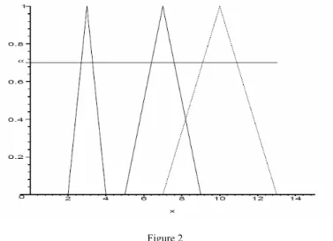
value. Fig. 2 demonstrates fuzzy addition with fuzzy numbers represented as lines. The dotted triangle number is the sum of the two other triangle numbers.

Figure 2 Fuzzy addition with

α

^-cut

This way we can have all the well-known unary (

−

x,

x

²) and binary operations (x

+

y,

xy

,

x mod y

) available as fuzzy operations. However the calculation of fuzzy operations with

α

-cut is tedious and often impractical. In this paper a new efficient method is proposed which is equivalent with the

α

-cut.

Fuzzy numbers are often composed of two strictly monotone functions, i.e. the left side denoted as

δ

_l, and the right side denoted as

δ

_r of the fuzzy number. Fuzzy operations can be carried out by first applying them to the left sides than to the right sides of the operands.

This separation allows us to treat fuzzy numbers as strictly monotone functions when dealing with fuzzy arithmetic operations. In the following we omit the subscript from

δ

_l and

δ

_r and simply write

δ

with the inherent assumption that we shall only do arithmetic operations with functions representing the same side of fuzzy numbers.

Lemma 2.1 Let

δ

₁

, δ

₂

, … , δ

_n (n

≥ 1

) be strictly monotone functions representing soft inequalities and let

F

be an n-ary fuzzy operation over them.

If

), , , , (

= F δ

₁

δ

₂

δ

_n

δ …

then

( )

(

⁻

^,

⁻

^{, ,}

⁻

)

⁻

^{( ) ⇐}

= )

( z F δ

₁ ¹

δ

₂ ¹

δ

_n ^{1 1}

z

δ …

(1)

{ ( ), ( ), , ( ) } . min

sup

= )

(

_{1 1 2 2}

= ) , 2, 1,

( n

n z x x x F

x x

x

z δ δ δ

δ …

…

Proof. It can be easily verified that the method is equivalent with the

α

-cut. □ Fig. 3 visualizes the equivalence for the addition of lines. The left side shows the result of lines added together using

α

-cut with the result presented as the dotted line. On the right side we have simply added together the inverse functions of the two operands. The result is also presented as a dotted line. It can be seen from the figures that the result of the

α

-cut is indeed the inverse of the result in the right hand side figure.

Figure 3

Left:

α

-cut addition, right: inverse of addition

We can state a theorem regarding the properties of fuzzy operations.

Theorem 2.2 Let

δ

₁

, δ

₂

, … , δ

_n (n

≥ 1

) be strictly monotone functions representing fuzzy inequalities and let

F

be an n-ary fuzzy operation over them.

If

(

2 ^{1 1}

)

1

1⁻

,

⁻

, ,

_n⁻ F

δ δ

…

δ

is strictly monotone then

F

has all the properties as its non-fuzzy interpretation.

Proof. It can be derived from Eq. 1 in Lemma 2.1. □

3 Additive Pliant

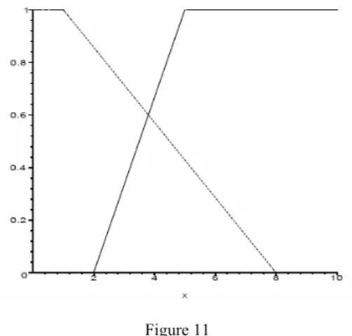
Triangle fuzzy numbers are commonly used to represent approximate values. A triangle fuzzy number has one line on each side. We can add triangle fuzzy numbers by first adding their left lines and than adding their right lines together.

Lemma 2.1 let us derive a general formula for adding lines.

Definition 3.1 We say that a line

l (x )

is given by its mean value if

2 ) 1 (

= )

( x m x − a + l

as shown in Fig. 4.

Figure 4

Line given by its mean value a and tangent

m = tan α

The inverse of

l (x )

denoted as

l

⁻¹

( y )

can be calculated easily

2 . 1

= )

1

(

m a y y

l − +

−

3.1 Addition

Theorem 3.2 Let

2 ) 1 (

= )

(

_i

−

_i

+

i

x m x a

l

(

i ∈ {1, … , n }

) lines given by their mean values. The fuzzy sum of

l

_i lines denoted as l is also a line and can be given as

2 ) 1 (

= ) ( )

(

= )

( x l

₁

x ⊕ ⊕ l x m x − a +

l …

_n

where

. 1 =

1 =

1

= 1

=

i n

i i n

i

a a m and

m

∑ ∑

Proof. Using Lemma 2.1 gives us

( ^{( ) ( )} )

= )

(

₁ ^{1 1}

1 y l y l y

l^{− −}

+… +

_n⁻

2 = 1 2 =

1

=

1

= 1

= 1

=

i n

i i n

i i i n

i

m a y m a

y

∑ ∑

∑ ⁺

⎟⎟

⎟ ⎟

⎠

⎞

⎜⎜

⎜ ⎜

⎝

⎛ −

⎟⎟

⎟ ⎟

⎠

⎞

⎜⎜

⎜ ⎜

⎝

⎛

− +

i n

i i n

i

m a y

^⎟ _⎠ ^⎞ ∑ ⁺ ∑

⎜ ⎝

⎛ −

1

= 1

=

1 2

= 1

From here we have

2 . 1 1

= 1 ) (

1

= 1

=

+

⎟ ⎠

⎜ ⎞

⎝

⎛ − ∑

∑

ⁱ

n

i i n

i

a x m x

l

Substituting

m

1

and a into the equation we get the desired result

( ) .

2

= 1 )

( x m x − a + l

□

3.2 Multiplication by Scalar

Theorem 3.3 Let

2 ) 1 (

= )

( x m x − a + l

line given by their mean values.

The scalar multiplication of the lines is:

2 ) 1 (

= )

( x m ′ x − a ′ + c: l

where

c m m ca

a ′ = ′ =

Proof. Using Lemma 2.1 gives us

2 . 1

= )

1

(

⎟⎟

⎟ ⎟

⎠

⎞

⎜⎜

⎜ ⎜

⎝

⎛

− +

− a

m y c x l

From here we have

2 . ) 1 (

= )

( x − ca +

c x m l 3.3 Subtraction

Calculations for subtraction yields

( ) .

2 ) 1 1 (

1

= 1

= )

(

_{1 2}

2 1 2

1

− − +

−

a a x m m l l x

l

Note: l does not exist when m₁

=

m₂.

It is an important property that the result of the operation is also a line, i.e. the operation is closed for lines.

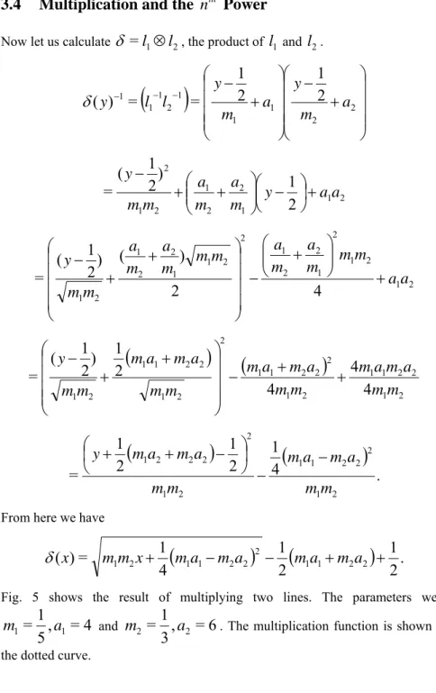
3.4 Multiplication and the n Power

^th

Now let us calculate

δ =

l₁

⊗

l₂, the product of l₁ and l₂.

( )

⎟⎟

⎟ ⎟

⎠

⎞

⎜⎜

⎜ ⎜

⎝

⎛

− +

⎟⎟

⎟ ⎟

⎠

⎞

⎜⎜

⎜ ⎜

⎝

⎛

− +

−

− −

2 2 1 1 1

2 1 1

1

2

1 2

1

=

= )

(

a

m y m a

y l

l

δ

y

2 1 1

2 2 1 2

1 2

2 ) 1

2 ( 1

= y a a

m a m

a m

m

y ⎟ +

⎠

⎜ ⎞

⎝ ⎛ −

⎟⎟ ⎠

⎜⎜ ⎞

⎝

⎛ +

− +

2 1 2 1 2

1 2 2 1 2 2 1 1 2 2 1

2

1

2 4

) ) (

2 ( 1

= a a

m m m

a m m a

m m a m

a m m

y ⎟⎟ ⎠ +

⎜⎜ ⎞

⎝

⎛ +

−

⎟ ⎟

⎟ ⎟

⎠

⎞

⎜ ⎜

⎜ ⎜

⎝

⎛ +

− +

( ) ( )

2 1

2 2 1 1 2

1 2 2 2 1 1 2

2 1

2 2 1 1

2

1

4

4 4

2 ) 1 2 ( 1

= m m

a m a m m

m a m a m m

m a m a m m

m

y − + +

⎟⎟

⎟ ⎟

⎠

⎞

⎜⎜

⎜ ⎜

⎝

⎛ +

− +

( ) ( )

4 . 1 2 1 2

1

=

2 1

2 2 2 1 1

2 1

2 2 2 2 1

m m

a m a m m

m a m a m

y −

−

⎟ ⎠

⎜ ⎞

⎝

⎛ + + −

From here we have

( ) ( ) .

2 1 2

1 4

= 1 )

(

x m₁m₂x

+

m₁a₁

−

m₂a₂ ²

−

m₁a₁

+

m₂a₂

+ δ

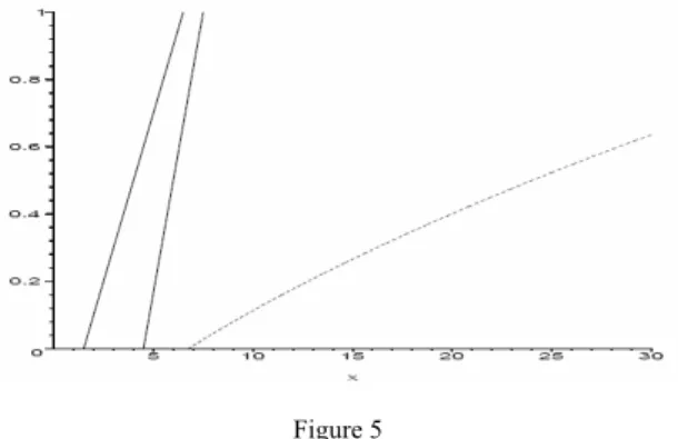
Fig. 5 shows the result of multiplying two lines. The parameters were

4

= 5 ,

= 1

₁

1

a

m

and

, = 6

3

= 1

₂

2

a

m

. The multiplication function is shown as the dotted curve.

Figure 5 Multiplication of lines

The result is not a line. We need to remain in the world of lines to be able to carry out further arithmetic operations. This can be achieved by approximating the result with a line, e.g. using the least squares method.

Let us calculate the

n

^th power of

2 ) 1 (

= )

( x m x − a +

l

.

( ^{( )} ) ^{= 2 1 .}

= )

(

^{1 1}

n

n

a

m y y

l y

⎟⎟

⎟ ⎟

⎠

⎞

⎜⎜

⎜ ⎜

⎝

⎛

− +

−

δ

−

From here we get

( ) ^.

2

= 1 )

( x m

ⁿ

x − a + δ

An approximation method should also be used here to get a line function from the result.

3.5 Properties of Operations

Theorem 3.4 Addition is commutative and associative over lines.

Proof. The properties can be easily seen from the construction of

m

1

and a in

Theorem 3.2. □

Theorem 3.5 Multiplication over lines is commutative, associative and distributive over addition.

Proof. Theorem 2.2 guarantees that these properties holds. □

4 Multiplicative Pliant

Let us start by introducing a special fuzzy inequality, the pliant inequality and examine its most important properties.

4.1 Pliant Inequality Model

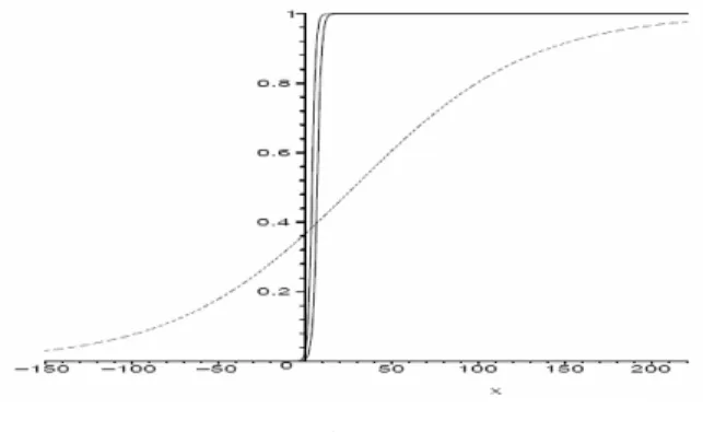
Definition 4.1 A pliant inequality is given as a sigmoid function of

) ( 1 =

= 1 }

<

{

_{( )} ^{( )}

x

x e

a

_{λ −λ x−a}

σ

_a^λ

+

where a is the mean value, i.e.

2

= 1 )

)

(

(_a^λ

a

σ

.

Figure 6

Pliant inequality with

λ = 0.7

and a

= 4

parameters

The following properties can be seen from the figure

<

a x

then

1

{ < } > , a

_λ

x 2

a

=

x then

1

{ < } = , a

_λ

a 2

a

>

x then

1

{ < } < . a

_λ

x 2

Definition 4.2 The inverse function of

σ

⁽_a^{λ )}

(

x

)

is denoted as

( ) ^σ

^{(aλ ) −1}

⁽

^x

⁾

^and

can be calculated easily. Let

, 1 =

= 1 )

(

_{( )}

)

(

ω

σ

_a^λ _{λ x a}

x e

_{− −}

+

then

) ( )

(

) =

(1

=

1 ω + e

^{−λ x−a}

ω + ω e

^{−λ x−a}

)

=

(

1

x a

e

^{− −}

−

_λ

ω ω

) ( 1 =

ln ⎟ − x − a

⎠

⎜ ⎞

⎝

⎛ − λ

ω ω

( ) ^{( ) = 1 ln 1 .}

=

^{( ) 1}

a

x

_a

⎟ +

⎠

⎜ ⎞

⎝

⎛ −

−

−

ω ω ω λ

σ

^λ

Definition 4.3 The first derivative of

σ

⁽_a^{λ )}

(

x

)

is denoted as

( ^σ

^{(aλ )}

⁽

^x

⁾ )

^{. The}

following properties hold

( ^σ

^{(aλ )}

^{( )} ) ^{= σ}

^{(aλ )}

^{( ) |}

^x=a

^{= 4 λ ;}

dx x d

a

depending on

λ

, if

λ > 0

then

( ^σ

^{(aλ )}

^{( ) x} )

^' is strictly monotone increasing,

λ = 0

then

( ^σ

^{(aλ )}

^{( ) x} )

^'

^{≡ 0,}

λ < 0

then

( ^σ

^{(aλ )}

^{( ) x} )

^' is strictly monotone decreasing.

When we apply an arithmetic operation to pliant inequalities we need to make sure that the operation is meaningful, i.e. the pliant inequalities represent the same sides of the fuzzy numbers. The following criteria formulates this requirement.

Criteria 4.4 If ^{( 2) ( )}

2 1) (

1

, , ,

ⁿ

an a

a

λ λ

λ

σ σ

σ …

are inputs to an n-ary fuzzy arithmetic operation then

) ( sgn

=

= ) ( sgn

= ) (

sgn λ

₁

λ

₂

… λ

_n

must always hold.

4.2 Addition

Theorem 4.5 Addition is closed over pliant inequalities and the addition function can be given as

1

=

^{( )}

) ( 1)

(

1

⊕ ⊕

ⁿ _a n

≥

an a

λ λ

λ

σ σ

σ

…

where

. 1 =

1 =

1

= 1

=

i n

i i n

i

a a

and

∑

∑ _λ

λ

Proof. We prove by induction, if i

= 1

then the statement is trivially true. Now let us assume that it holds for i

=

n

− 1

and prove it for

i = n

,

) ) (

) ( (

) (

1) (

1 1)

(

1

=

=

ⁿ

an a

n an a

n an a

λ λ λ

σ λ

λ

λ

σ σ σ σ

σ

δ ⊕ ⊕ ⊕

_′^′

⊕

′′

−

… −

where

. 1 =

1 =

¹

1

= 1

1

=

i n

i i n

i

a a

and

∑

∑

⁻

^′

⁻

′ λ

λ

Now by using Lemma 2.1 we have

( ) ^{( )} ( ) ^{( ) =}

= )

(

^{( ) 1 ( ) 1}

1 z z ⁿ z

an a

− −

′

−

σ

^λ′

+ σ

^λ

δ

1 = 1 ln ln 1

= 1

_n

n

z a a z

z

z

⎟ +

⎠

⎜ ⎞

⎝

⎛ − + −

+ ′

⎟ ⎠

⎜ ⎞

⎝

⎛ −

− λ ′ λ

= ) 1 (

1 ln

= 1

¹

1

= 1

1

=

n i n

n i i n

i

a z a

z

⎟ + +

⎠

⎜ ⎞

⎝

⎟⎟ ⎛ −

⎠

⎜⎜ ⎞

⎝

⎛

+ −

− ∑

∑

⁻

_{λ λ}

⁻

1 . 1 ln

= a

z z ⎟ +

⎠

⎜ ⎞

⎝

⎛ −

− λ

⁽²⁾

If

1 0

1

=

≠

∑

i n

i

λ

^then

^{( )}

1

z

δ

− is a strictly monotone function and inverse of a pliant inequality. Therefore

δ (x )

is a pliant inequality with

λ

and a parameters:

( ) ^{= ( ).}

)) ( ( 1

= 1 ) (

= )

(

^{(1) ( ) ( )}

1

x

a x x e

x

ⁿ _a

an a

λ λ

λ

σ

λ

σ

σ

δ ⊕ … ⊕ +

₋

−

(3)

If

1 = 0

1

= i n

i

λ

∑

then the addition function does not exist since

δ

⁻¹

( z ) = a

is a

constant thus has no inverse. □

4.3 Multiplication by Scalar

Theorem 4.6 Let given

σ

⁽_a^{λ )}

(

x

)

sigmoid function.

The scalar multiplication of the sigmoid function is:

) (

= )

(

^{( )}

)

( x x

c:

σ

_a^λ

σ

_a^λ_′^′

where

ca

c a =

= ′

′ λ λ

Proof. Using Lemma 2.1 gives us

( ) _⎟⎟

⎠

⎜⎜ ⎞

⎝

⎛ ⎟ +

⎠

⎜ ⎞

⎝

− ⎛ −

−

x a c x

a

x

ln 1

= 1 )

(

¹

) (

σ

^λ

λ

From here we have

) ) (

( )

(

1

= 1 1

= 1 )

(

_{x a}

ca c x

a

e

e

x

_{− ′ − ′}

−

−

′

′

+

+

^{λ λ}

σ

λ

□

4.4 Subtraction

We can derive subtraction from addition and negation.

Lemma 4.7 Negation is closed over pliant inequalities and the negation function can be given as

) ) (

(^λ

= σ

^λ

σ

_{a −a}⁻

Proof. Let

)

= σ

(^λ

δ

_a by using Lemma 2.1 we have

( ) ^{( ) =}

= )

(

^{( ) 1}

1

⎟

⎠

⎜ ⎞

⎝

− ⎛

⁻

−

z σ

_a^λ

z

δ

).

1 ( 1 ln 1 =

1 ln

= a

z a z

z

z ⎟ + −

⎠

⎜ ⎞

⎝

⎛ −

− −

⎟ −

⎠

⎜ ⎞

⎝

⎛ −

λ λ

Therefore

).

( 1 =

= 1 ) (

= )

(

^{( )} _{( )( ( ))} ^{( )}

x

x e

x σ

_a^λ _{λ x a}

σ

_a^λ

δ

_{−− −− −}⁻

+

(4)

□ Theorem 4.8 Subtraction is closed over pliant inequalities and the subtraction function can be given as

.

=

²

1 1 1

2 1 2) (

2 1) (

1

⎟⎟

⎠

⎞

⎜⎜

⎝

⎛ −

− λ λ λ

λ

σ σ

σ

_a

_{a a a}

Proof. Let

2) (

2 1) (

= σ

1^λ

σ

^λ

δ

_a

_a

by using Lemma 2.1 and Lemma 4.7 we have

( ) ( ) ⁼

=

^{( 2) 1}

2 ) 1

( 1 1

1 − −

−

σ

^λ

− σ

^λ

δ

_{a a}

( ) ( ) ⁼

=

^{( 2) 1}

2 ) 1

( 1

1

⎟

⎠ ⎞

⎜ ⎝

+ ⎛−

⁻

− λ

λ

σ

σ

_{a a}

( ) ( ) ⁼

=

^{( 2) 1}

2 ) 1

( 1 1

−

−

+

^λ

λ

σ

σ

_{a a}

( )

( ) ^,

=

^{( 2) 1}

2 1)

( 1

⊕

^λ −

λ

σ

σ

_{a a} therefore

( ^σ

⁽a^λ₁¹⁾

^σ

⁽a^λ₂²⁾

) ^{= σ}

⁽a₁^λ1)

⊕ ( ^σ

⁽a^λ₂²⁾

) ^.

(5)

Substituting Eq. 4 and Eq. 3 into Eq. 5 we get the desired result

(

⁽₁^{1) (}₂²⁾

) ⁼

⁽₁^{1) (} ₂²⁾

⁼

^⎜⎜⎝⎛₁¹¹−⁻₂^{12⎟⎟⎠⎞}

^.

−

⊕

−^{λ λ λ}

λ λ

λ

σ σ σ σ

σ

_a

_{a a a a a} (6)

□ Note: The function does not exist in case of

λ

₁

− λ

₂

= 0

.

4.5 Multiplication and the n Power

^th

Now let ^{( 2)}

2 1) (

= σ

^λ1

σ

^λ

δ

_a

⊗

_a . By using Lemma 2.1 we get

( ) ^{( )} ( ) ^{( ) =}

= )

(

^{( 2) 1}

2 ) 1

( 1 1

1

⎥⎦ ⎤

⎢⎣ ⎡

⎥⎦ ⎤

⎢⎣ ⎡

^{− −}

−

z σ

_a^λ

z σ

_a^λ

z

δ

1 = 1 ln ln 1

= 1

₂

2 1 1

⎥ ⎦

⎢ ⎤

⎣

⎡ ⎟ +

⎠

⎜ ⎞

⎝

⎛ −

⎥ −

⎦

⎢ ⎤

⎣

⎡ ⎟ +

⎠

⎜ ⎞

⎝

⎛ −

−

a

z a z

z z

λ λ

2 1 2

1 1 2 2

2 1

ln 1 ln 1

= 1

aa

z z a

a z

z

⎟ +

⎠

⎜ ⎞

⎝

⎟⎟ ⎛ −

⎠

⎜⎜ ⎞

⎝

⎛ + − + −

⎟ ⎠

⎜ ⎞

⎝

⎛ −

λ λ λ

λ

2 1 2

1 2 2 1 1 2

2 1

ln 1 ln 1

= 1

aa

z z a

a z

z

⎟ +

⎠

⎜ ⎞

⎝ + ⎛ −

⎟ −

⎠

⎜ ⎞

⎝

⎛ −

λ λ

λ λ λ

λ

⁽⁷⁾

Unfortunately this is not an inverse pliant inequality and it is not monotone. To obtain the roots of the function we set

( )

⁽a₁^{1) 1}

⁽

^z

^{) = 0}

λ −

σ

to get

1 0 1

1

= 1

_a

e

z

_λ

+

and we set

( ) ^σ

^(aλ₂^{2) −1}

⁽

^z

^{) = 0}

^{to get} 1 _{2 2}

1

= 1

_a

e

z

_λ

+

^.

A complete analysis of

δ

⁻¹ would require checking both the

λ

₁

λ

₂

> 0

and

0

2

<

1

λ

λ

cases. However by Criteria 4.4 we only need to examine the first case.

Let

λ

₁

λ

₂

> 0

. In this case

δ

⁻¹

( z ) < 0

when

z ∈ ( min ( z

₀

, z

₁

), max ( z

₀

, z

₁

))

. By using the first derivative we get

2) 2 1 ( 1 2 1

1

= 1

a min a

e

z

λ +λ

+

. Let us transform Eq.

7 to get

z

on the left side of the equation

x a z a

z a

a z

z

1 =

1 ln 1 ln

2 1 2

1 2 2 1 1 2

2 1

⎟ +

⎠

⎜ ⎞

⎝ + ⎛ −

⎟ −

⎠

⎜ ⎞

⎝

⎛ −

λ λ

λ λ λ

λ

( ) =

2 1 ln 1

1

²

2 2 1 1 2

1

⎟⎟

⎠

⎜⎜ ⎞

⎝

⎛ ⎟ − +

⎠

⎜ ⎞

⎝

⎛ − a a

z

z λ λ

λ λ

(

1 1 2 2

)

²

1 2

4

1 2

a a

x a a λ λ

λ λ

− + +

(

_{1 1 2 2}

)

² _{1 2}

(

_{1 1 2 2}

)

²

4

= 1 2

1

ln 1 a a x a a

z

z λ λ ⎟⎟ ⎠ λ λ + λ − λ

⎜⎜ ⎞

⎝

⎛ ⎟ − +

⎠

⎜ ⎞

⎝

⎛ −

(

_{1 1 2 2}

)

_{1 2}

(

_{1 1 2 2}

)

²

4

= 1 2

1

ln 1 a a x a a

z

z ⎟ − λ + λ ± λ λ + λ − λ

⎠

⎜ ⎞

⎝

⎛ −

(8)

We need to check two cases here. First, let

z ∈ (0, z

_min

]

. In this case

δ

⁻¹

( z )

is strictly monotone decreasing (thus has an inverse) and the left side of Eq. 8 is positive therefore

( ) ( ) .

4

= 1 2

1

ln 1

₁

a

_{1 2}

a

_{2 1 2}

x

₁

a

_{1 2}

a

₂ ²

z

z ⎟ − λ + λ λ λ + λ − λ

⎠

⎜ ⎞

⎝

⎛ −

From here we have

(

_{1 1 2 2}

)

²

(

_{1 1 2 2}

)

2

1

2

1 4

= 1

ln 1 x a a a a

z

z ⎟ λ λ + λ − λ + λ + λ

⎠

⎜ ⎞

⎝

⎛ −

( ) ( )

_⎟⎟

⎠

⎞

⎜⎜⎝

⎛ + − + +

−

2 ^{11 2 2}

2 1 2 2 1 4 1 2 1

=

1

1

^{x a a a a}

z e

z ^{λλ λ λ λ λ}

( ) ( )

_⎟⎟

⎠

⎞

⎜⎜⎝

⎛ + − + +

+

^{2 11 2 2}

2 1 2 2 1 4 1 1 2

1

1

= 1

a a a a x

e z

λ λ λ

λ λ λ

For

(

⁽a₁^{1) (}a₂²⁾

) ^{( x )}

λ

λ

σ

σ ⊗

this gives us

( ) _{( ) ( )}

⎟⎟⎠

⎞

⎜⎜⎝

⎛ + − + +

+

⊗

2 2 1 2 1 2 1 2 2 1 4 1 2 1 1 2)

( 2 1) (

1 '

1

= 1 ) (

= ) (

a a a a x a

a

e x

x

λ λ λ

λ λ λ λ

λ

σ

σ δ

which is not a pliant inequality though rather similar. The domain of

δ

^'

( x )

is

) 2 ,

[ 1

2 2 2 1 1 2 1

⎟ ∞

⎠

⎜ ⎞

⎝

⎛ −

−

∈ λ λ

λ λ

a

x a .

For the second case we have

z ∈ [ z

_min

,1)

. Now

δ

⁻¹

( z )

is strictly monotone increasing (thus has an inverse) and the left side of Eq. 8 is negative. Now we have

(

_{1 1 2 2}

)

²

(

_{1 1 2 2}

)

2

1

2

1 4

= 1

ln 1 x a a a a

z

z ⎟ − λ λ + λ − λ + λ + λ

⎠

⎜ ⎞

⎝

⎛ −

( ) ( )

_⎟⎟

⎠

⎜⎜ ⎞

⎝

⎛− + − + +

−

2 ^{11 2 2}

2 1 2 2 1 4 1 1 2

=

1

1

^{x a a a a}

z e

z ^{λλ λ λ λ λ}

( ) ( )

_⎟⎟

⎠

⎞

⎜⎜⎝

⎛− + − + +

+

^{2 11 2 2}

2 1 2 2 1 4 1 2 1

1

1

= 1

a a a a x

e z

λ λ λ

λ λ λ

For

(

⁽a₁^{1) (}a₂²⁾

) ^{( x )}

λ

λ

σ

σ ⊗

we get

( ) _{( ) ( )}

⎟⎟⎠

⎞

⎜⎜⎝

⎛− + − + +

′

+

⊗

2 2 1 2 1 2 1 2 2 1 4 1 2 1 1 2)

( 2 1) (

1 '

1

= 1 ) (

= ) (

a a a a x a

a

e x

x

λ λ λ

λ λ λ λ

λ

σ

σ δ

The domain of

δ

^'′ is

, )

2 [ 1

2 2 2 1 1 2 1

⎟ ∞

⎠

⎜ ⎞

⎝

⎛ −

−

∈ λ λ

λ λ

a

x a .

Note that here

λ

_i and

a

_i play the analogous roles of

m

_i and

a

_i in additive pliant multiplication.

Functions

σ

^' and

σ

^'′ shall be used if we need to multiply pliant inequalities from the positive range of the x axis. If

λ

₁

, λ

₂

< 0

then

σ

^' should be used because it maps the positive part of ^{( 1)}

1

σ

_aλ and ^{( 2)}

2

σ

_aλ . If

λ

₁

, λ

₂

> 0

then

σ

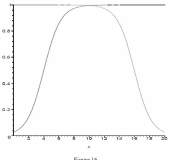
^'′ should be used.

Fig. 7 demonstrates multiplication of ^{( 1)}

1

σ

_aλ and ^{( 2)}

2

σ

_aλ pliant inequalities. The parameters of the operands were

λ

₁

= 0.9,

a₁

= 4

and

λ

₂

= 0.8,

a₂

= 7

respectively. The result is shown as the dotted curve.

Figure 7

Multiplication of pliant inequalities

The calculations show that multiplication is not closed for pliant inequalities.

Nevertheless we can approximate the result well with a pliant inequality. We construct this function to take the value

2

1

at a₁a₂ and let the tangent here be the

same as of the multiplication function. For the tangent we have

1 2 2 1

1 4 1

λ λ

a a +

, and

our approximation function is

.

1 2 2 1 1 4 1

2 1 2) (

2 1) (

1

⎟⎟

⎟⎟

⎟

⎠

⎞

⎜⎜

⎜⎜

⎜

⎝

⎛

≈

+

⊗

^{λ λ λ}

λ

σ σ

σ

a a a a a

a

Fig. 8 shows the approximation of the multiplication in Fig. 7. The approximating pliant inequality is plotted as the dotted curve.

Figure 8