The Impact of Adverse Selection on Stock Exchange Specialists’ Price Quotation Strategy*

The Impact of Adverse Selection on Stock Exchange Specialists’ Price Quotation Strategy*

Kira Muratov-Szabó – Kata Váradi

This paper focuses on the activity of the specialists – one of the key participants in stock exchange trading. We attempt to model the price quotations of specialists in a modelling framework where some of the parties involved in the transactions may be informed, while others are uninformed “liquidity traders”. It is in this adverse selection modelling framework that, relying on the technique of Monte Carlo simulation, we seek an answer to the following research questions: how does adverse selection impact the price quotation of specialists; to what extent are prices and logreturns influenced by uncertainty; to what degree of accuracy can specialists determine the proportion of informed traders and liquidity traders from trading volumes? Our model confirmed that as soon as uncertainty subsided in the simulated market, the number of transactions, wealth and the stock portfolio started to grow, while price fluctuations began to decline and the standard deviation and the distribution of logreturns edged closer and closer to a normal distribution, which points to improving market efficiency.

Journal of Economic Literature (JEL) codes: G12, G14, G17 Keywords: specialist, price quotation, adverse selection

1. Introduction

In this study, we explore the price quotation strategy of stock exchange specialists.

Specialists are market makers in stock exchange trading with exclusive rights to quote bid and ask prices in a given product. The study is based, on the one hand, on a paper by Kornis (2017) that focused on the behaviour and presumed strategies of specialists in quote-driven markets, which we supplemented with the inclusion of quoted volume. On the other hand, the article by Caglio and Kavajecz (2006) also serves as a basis for our study, as the authors demonstrate that specialists can use quoted volumes strategically to mitigate the risk of adverse selection. The concept of adverse selection is presented in this study as a scenario where some

* The papers in this issue contain the views of the authors which are not necessarily the same as the official views of the Magyar Nemzeti Bank.

Kira Muratov-Szabó is currently a Graduate student at Corvinus University of Budapest. This study is based on her thesis submitted in the academic year of 2017/2018. Email: muratov.kira@gmail.com

Kata Váradi is an Associate Professor at Corvinus University of Budapest. Email: kata.varadi@uni-corvinus.hu The Hungarian manuscript was received on 24 September 2018.

of the market participants placing orders are informed about the expected price movement of the product, while others are uninformed and act as liquidity traders.

However, when posting the prices the specialist has no way of knowing whether the actor placing the order is informed or not; consequently, he does not know which specific price should be quoted. Overall, our study connects these two research papers, and the new model we construct is intended to seek an answer to the following research questions:

• How does adverse selection impact the specialist’s price quotation?

• How do prices and logreturns change at various uncertainty levels?

• How precisely can specialists update their belief regarding the proportion of informed traders based on transaction volume?

Drawing partly from the work of Caglio and Kavajecz (2006) and partly from Kornis (2017), our model includes numerous new assumptions and new methods. The former study primarily provided a theoretical background, while the latter inspired ideas in the area of practical execution. In order to simulate the model, we created a programme¹ in Excel in the Visual Basic for Applications programming language.

After the introduction, in the second section of the study we provide an overview of the relevant international literature. The third section presents the model proposed by Caglio and Kavajecz (2006) supplemented with our own additions and methods. We attempt to explore possible ways of introducing the problem of adverse selection into the model and examine who exactly acts as informed traders, who are liquidity traders, and how can specialists identify them in order to maximise their profits. In the fourth section, we briefly describe the simulation process as a preparation for the fifth section, which is dedicated to the statistical analysis of the results yielded by the simulation as a reward for our practical work.

In Section 5 we also present our figures and our conclusions. The study is concluded with a summary in which we offer concise answers to the questions posed in the introduction.

2. Literature review

Although the approaches taken may be different, a substantial part of the research on financial markets ultimately seeks an answer to the same question: in what way can market prices be predicted in order to serve as a basis for a profitable trading strategy? The literature on market microstructure has shed new light on this area in recent decades: instead of concentrating on actual price movements to draw

1 The codes of the programme’s main components (subroutines and functions) are presented in the Appendices.

conclusions about expected price developments, this field of study attempts to determine how specific market mechanisms affect the price discovery process.

Market microstructure research examines who market participants are, what level of information they have and what type of products are being traded (e.g.

underlying instruments or derivatives); in other words, it tries to investigate market efficiency and price formation based on the elements of market microstructure (O’Hara 1995).

One central concept in market microstructure is market liquidity. Market liquidity is understood as the speed at which a given product can be sold or purchased in a given volume with the smallest possible price effect. This issue is generally approached both by practitioners and scientific research by way of the bid-ask spread, a measure of liquidity’s transaction cost expressing the difference between the best bid price and ask price. Based on Foucault et al. (2013), a basic premise of market microstructure is that the bid-ask spread is composed of 1) adverse selection, 2) inventory control and 3) order-processing costs (Figure 1) as indeed, specialists face these costs in trading and pass on these costs to market participants when quoting prices.

1. Adverse selection cost: Since informed traders purchase when the quoted price is too low and sell when the quoted price is too high based on market information, specialists are exposed to adverse selection costs.

Figure 1

Components of transaction costs

Excepted transaction price after an order at time t

t Time

Order-processing cost component

Adverse selection cost component Inventory control cost component

Source: Foucault et al. (2013), p. 121.

2. Inventory control cost: On continuous markets buy and sell orders are not received at one and the same time, which leads to a temporary disparity between the offers. In such cases, specialists step in committing their own inventory in order to restore equilibrium between supply and demand, while their net position remains zero over time. This role, however, exposes specialists to inventory control risk as the value of their inventory may change at any time, for example as a result of new information or intelligence affecting the given asset. For this reason, specialists charge inventory control costs.

3. Order-processing cost: Specialists charge order-processing costs for trading commissions, for the clearing and settlement fees, paperwork, time spent on the phone and such.

On the whole, these costs are ultimately charged to the rest of the market participants in the form of transaction costs, which is the bid-ask spread itself (Foucault et al. 2013).

The problem of transaction costs was first formalised by Demsetz (1968). Harold Demsetz treated the bid-ask spread as a cost assumed by the trader for immediacy.

Bagehot (1971) asserted that there are (at least) two kinds of traders who confront specialists: informed traders and liquidity-motivated traders. Informed traders possess non-public information that allows them to have a better estimate of the future price of a security than liquidity traders or specialists themselves. Since transactors trading on special information always have the option of not trading with the specialists, the specialists will never gain from them; they can only lose. By contrast, transactions with liquidity-motivated traders can be profitable, as these market participants are willing to pay a “fee” for gaining access to immediacy.

These two thoughts are synthesised by Copeland and Galai (1983) who modelled the bid-ask spread as a “trade-off”, which compensates specialists for the expected losses to informed traders with the expected gains from liquidity traders. The research by Glosten and Milgrom (1985) was founded on this concept. The authors used a formal model to demonstrate that the spread increases in response to adverse selection. They assume that specialists are risk-neutral, competitive and make zero expected profits. In addition, specialists are assumed to have unlimited inventories of both money and securities. From their research Kornis (2017) drew the following five key assumptions:

• The bid and ask prices straddle the price that would prevail if all traders had the exact same information as the specialists.

• The prices at which transactions actually occur form a martingale.²

2 For more detail about martingale processes, see: Doob (1971)

• There is a boundary on the size of the spread that can arise from adverse selection.

• The price expectations of the specialists and informed traders tend to converge.

• Generally, ask prices increase and bid prices decrease if the insiders’ information becomes better, or the insiders become more numerous relative to liquidity traders, or when the elasticity of the expected supply and demand of a liquidity trader increases.

All of the literature discussed so far focused on the size of the bid-ask spread. As Harris (1990a) pointed out, however, the spread is only one dimension of market liquidity. Harris (1990a) defined liquidity as follows: “A liquid market is one in which every agent can buy and sell at any time a large quantity rapidly at low cost. Liquidity is a trader’s willingness to take the opposite side of a trade that is initiated by someone else when the cost is low enough.” In other words, in addition to the bid-ask spread, turnover can also be a measure of liquidity. A consistent summary of liquidity measures was provided, for the first time, by von Wyss (2004).

On the NYSE (New York Stock Exchange) the full offer of a specialist includes both the best bid and the best ask prices, as well as the volume of shares available at the best price, in other words, the depth. If the specialist perceives an increased probability of insider information among certain traders, he can respond by widening the bid-ask spread. Alternatively, he can protect himself by offering a lower trading volume at each quoted price (Lee et al. 1993).

It was a paper by Kyle (1985) that first defined liquidity by using the concepts of tightness, depth, breadth (static dimensions) and market resiliency (dynamic dimension). The (also dynamic) dimension of immediacy can be linked to Harris (1990b), while diversity was first identified as a new, separate dimension by Kutas and Végh (2005). In view of the multidimensional nature of market liquidity, it is highly surprising that much of the literature focuses on the spread alone. Numerous price quotation models examined in the context of adverse selection disregard depth with the proviso that all transactions (and hence the quotes) should be conducted in the same volume. Examples include the models presented in Copeland and Galai (1983), Glosten and Milgrom (1985) and Easley and O’Hara (1992). The models that permit trading in different volumes – such as those proposed by Kyle (1985) and Rock (1989) – typically assume that the specialist’s quotes are full quotes. In these models information on both the price and the volume is needed to support an implicit evaluation of the liquidity of the price quotation.

Lee et al. (1993) demonstrated that specialists can actively manage the risk of information asymmetry by adjusting both spreads and depths. Their result underscores the importance of the quantity dimension ignored by previous models and emphasises the fact that both spread and depth are needed to induce changes

in liquidity unambiguously. In other words, a widening (narrowing) of the spread, combined with a decrease (increase) in depth, is sufficient to induce a decrease (increase) in liquidity.

Similarly, Kavajecz (1999) investigated the reduction of adverse selection risk, and he did so from the angle of quoted depth. Four important conclusions may be drawn from his findings:

• If a quote changes, the specialist will (also) change the quoted volume in 90 per cent of the cases; in fact, the quote will only change in terms of volume in 50 per cent of the cases, with no shift in the price whatsoever. Consequently, the specialist actively manages his own inventory even if no price change occurs.

• If informed traders are in an overwhelming majority on the market, the specialist’s quotation is likely to reflect the top of the order book instead of his own inventory.

This is how he ensures that an incoming limit order will be matched with the best limit orders contained in the order book rather than being filled from his own inventory.

• Quoted volumes are consistent with the size of the specialist’s own stock portfolio;

consequently, determining the volume also plays a role in his strategy.

• In response to the announcement of new information, both the specialist and the traders decrease the volume of their orders.

Carrying this thought forward, the stylised theoretical framework in the article of Dupont (2000) shows that a risk-neutral, monopolistic specialist narrows quoted depth in proportion to the widening of the spread when he reacts to an increase in adverse selection; in other words, equilibrium depth is proportionally more sensitive than the spread to changes in the degree of adverse selection.

The elasticity of substitution between depth and spread – in consideration of the quality of information possessed by the better informed trader – depends on market conditions which, in turn, are determined by the information asymmetry, the asset’s volatility and the strength of demand for liquidity. This elasticity converges to infinity if market conditions become either extremely favourable (depth increases to infinity while the spread remains positive) or extremely unfavourable (depth approaches zero, while the spread remains finite). Whether the informed trader is risk-neutral or risk-averse does not essentially affect the results.

Kavajecz and Odders-White (2001) examined how specialists update their price schedules in a simultaneous equations model. They found that changes in the best prices and depths on the order book had a significant impact on the posted price schedule, while the effects of transactions and order activity were secondary.

Moreover, they pointed out that specialists revise quoted prices and quoted volumes

differently. For example, quoted depths are revised in response to transactions of any size, whereas the quoted prices are revised only when transaction sizes exceed the quoted depth. However, they found no evidence that specialists revise the price schedule in response to changes in their inventory.

Caglio and Kavajecz (2006) were the first to examine whether adjusting liquidity’s quantitative dimension, i.e. depth, gives rise to a specification error in the spread decomposition model. The aim is to understand whether changes in the bid-ask spread alone are capable of defining the size of the adverse selection. In other words: is the extent of the change in depth redundant information in decomposition procedures?

The authors constructed a simple sequential trade model, which offers a distinct, analytical solution to the specialist’s optimisation problem, i.e. how to choose prices and depths in order to maximise his profits. The model measures the changes induced at various levels of informed trading in the adverse selection component of the spread. The authors demonstrated that specialists can use quoted volume strategically to address adverse selection risk and the risk of change in the trading environment. The result is consistent with the previously mentioned finding (Kavajecz 1999) that a change in the quote will prompt the specialist – in roughly 50 per cent of the cases – to change the quoted volume, but not the price. The authors simulated the model based on this theoretical framework, examining two scenarios. In one scenario the specialist is not constrained by restrictions in terms of price quotation, while in the other scenario quoted volumes are constrained by the maximum limit on liquidity trading. Applying a simulated sequence, they compared the estimates of three decomposition models for the two scenarios. They found that spread decompositions failed to capture the full extent of adverse selection risk when the specialist could define depth without constraint. The solution is for researchers to use adverse selection measures that account for depth as well as spread to mitigate this problem.

3. The model

The basis of the model is the paper written by Caglio and Kavajecz (2006), which we supplemented with a number of new elements and methods:

1. Consistent with the assumption of Caglio and Kavajecz (2006):

a. we assume that the distributions, such as the distribution of the return on the asset under review, are normal.

b. we select the parameter values (such as quantitative data).

2. Our own, new assumptions for the specialist’s passive quotes are the following:

a. based on the current size of the bid-ask spread, the specialist needs to improve his quote depending on whether he has exceeded a pre-defined limit or not.

3. We connect the model with Kornis (2017) and run a simulation based on the result.

Consistent with Caglio and Kavajecz (2006), the analytical framework is the following: Consider a sequential trade model where the return on a risky asset is expressed by a stochastic variable of ϴ. As the authors did not define the distribution of the asset’s returns, we assume ϴ to have normal distribution, an expected value of 100 and a standard deviation of 5. At a probability of µ, the ultimate value of the security is ϴ₁, and at a probability of 1–µ it is ϴ₂, where ϴ₁ < ϴ₂. We conducted the simulation for five different µ values: 0.49³; 0.4; 0.3; 0.2 and 0.1.

Traders are uniformly distributed over the [0, 1] interval, with λ part of the traders being fully informed about the security’s return and 1–λ part of them not possessing any information about the ultimate value of the risky asset, where 0 < λ < 1. We took 0.2 to be the value of λ for the simulation.

Apart from traders, there is one actor on the market: the risk-neutral, profit maximiser specialist who posts the quote of the risky asset for his own purposes while also observing market rules. His task is to announce a bid price and size and an ask price and size set. No transaction takes place at prices and sizes worse than the announced set. In addition, the specialist has an expectation about λ, and he updates this belief after each trade, which is marked by λ_s.

3.1. Events of a period

Caglio and Kavajecz (2006) defined a period as follows. First, the two different return potentials of the risky asset change. Next, the specialist determines the quoted bid and ask prices (marked by b and a, respectively, where b < a in equilibrium) along with the corresponding bid and ask volumes (marked by β and α, respectively). While doing so, the specialist considers the probability of trading with the different traders, the volumes they are willing to purchase of the given financial product, the potential returns on the given product and the product’s expected value. Among the population of market participants, a randomly selected person decides whether he wants to trade or not. If the trader decides to trade, he selects a certain volume, which is either smaller than or equal to the relevant depth. After the transaction has been completed, the specialist updates his belief about the proportion of informed traders and revises its quoted offer. After he has defined his new offer, another trading round takes place, and this process is repeated again and again throughout a specific period.

3 We must use 0.49 instead of 0.5 in order to avoid dividing by 0 later on, such as in the case of Equation 4.

Caglio and Kavajecz (2006) assumed that each trader has only one trading opportunity. Since an informed trader has perfect information about the ultimate value of the risky asset, theoretically he can have infinite demand if the specialist has mispriced the asset. Only the specialist’s quoted volumes can put a limit on this demand; therefore, the key assumption of the model is that informed traders will choose maximum depth. Consequently, the j^th informed trader will place his order as follows:

qij= −β, ha b>θ^∗ α, ha a<θ^∗

⎧⎨

⎪

⎩⎪

(1) where ϴ^* is the real value of the risky asset and q stands for the volume. It should be noted that, since the specialist buys (sells) at the bid (ask) prices, the bid depth is positive and the ask depth is negative, i.e. βj > 0 and αj < 0.

Since uninformed traders are not driven by information, they can be viewed as a group of people with various, exogenously determined motivations and inclinations towards trading. The k^th trader is written as a set of (ek, rk), which represents the trader’s endowment and his reservation price. The positive (negative) values of ek mean that the trader wishes to sell (buy) a certain quantity of the risky asset. Moreover, a high (low) value of r_k indicates that the trader overvalues (undervalues) the asset. Therefore, each uninformed trader places an order in accordance with the following strategy:

q_k^u=

−min

[

]

+min⎡⎣α, ek ⎤⎦, if ek<0 and a<r_k

0, otherwise

⎧

⎨⎪

⎩⎪ (2)

Accordingly, an uninformed trader will buy (sell) if his reservation price is higher (lower) than the quoted ask (bid) price and the traded volume is the same as the ask (bid) depth or lower. For the sake of clarity, the volumes to be bought/sold by traders are uniformly distributed over a pre-fixed t₁ and t₂ set, and the reservation prices are also uniformly distributed between ϴ₁ and ϴ₂; accordingly:

e_k∼U t

[

]

[

]

Since they were not given, we took the interval of the fixed t₁ and t₂ set as [–100, 100], and the rk-s fall between two possible returns on the risky asset that are generated by the model from a normal distribution as described above. Moreover, suppose that both the ek-s and the rk-s are independent of each other.

Taking the two different trading strategies together, Caglio and Kavajecz (2006) calculated the way in which the specialist maximises the expected value of his profits as follows:

E_⎡⎣π

(

)

(

)

(

)

(

)

+

(

)

2−t₁

⎛

⎝⎜

⎞

⎠⎟

b−θ₁ θ₂−θ₁

⎛

⎝⎜

⎞

⎠⎟β µ θ

{ (

)

(

) (

) }

+

(

)

2−t₁

⎛

⎝⎜

⎞

⎠⎟

b−θ₁ θ₂−θ₁

⎛

⎝⎜

⎞

⎠⎟

1 2β

⎛⎝⎜ ⎞

⎠⎟

{

(

)

(

) (

) }

+

(

)

2−t₁

⎛

⎝⎜

⎞

⎠⎟

θ₂−a θ₂−θ₁

⎛

⎝⎜

⎞

⎠⎟α θ

{ (

)

(

) (

) }

+

(

)

2−t1

⎛

⎝⎜

⎞

⎠⎟

θ₂−a θ₂−θ₁

⎛

⎝⎜

⎞

⎠⎟

1 2α

⎛⎝⎜ ⎞

⎠⎟

{

(

)

(

) (

) }

(4)

The first line of the right-hand side of the equation indicates expected losses from transactions with informed traders, while the rest of the lines show the expected value of profitable or non-profitable trades with uninformed traders.

This optimisation makes implicit assumptions about the relationship between the variables chosen by the specialist. These assumptions can be summarised in the following two constraints:

1) Quoted depth is equal to or lower than maximum liquidity trading.

t₁≤α< 0 <β≤t₂ (5)

2) Quoted prices must fall between the two final returns:

θ₁<b<a<θ₂ ⁽⁶⁾ 3.2. The active quotation method

Caglio and Kavajecz (2006) defined the equilibrium values of the model as follows:

Proposition 1: If µ meets the following conditions:

λ−λ

( )

1−λ

( )

⎛

⎝⎜

⎜

⎞

⎠⎟

⎟<µ< 1−λ 1−λ

( )

⎛

⎝⎜

⎜

⎞

⎠⎟

⎟ (7)

then the unique equilibrium of the single-period model is:

b_u^*=1

4

(

[ ]

)

⁽

^{) (}

⁾

2

⎛

⎝⎜

⎞

⎠⎟

λ 1−λ

⎛⎝⎜ ⎞

⎠⎟ µ 1−µ

⎛

⎝⎜

⎞

⎠⎟

(

)

2t₂−1

2t₂ 1+ 8 t₂

⎛

⎝⎜

⎞

⎠⎟

λ 1−λ

⎛⎝⎜ ⎞

⎠⎟ µ 1−µ

⎛

⎝⎜

⎞

⎠⎟

(

)

a_u^*=1

4

(

[ ]

)

⁽

⁾

1

⎛

⎝⎜

⎞

⎠⎟

λ 1−λ

⎛⎝⎜ ⎞

⎠⎟ 1−µ µ

⎛

⎝⎜

⎞

⎠⎟

(

)

αu*=3 2t₁−1

2t₁ 1− 8 t₁

⎛

⎝⎜

⎞

⎠⎟

λ 1−λ

⎛⎝⎜ ⎞

⎠⎟ 1−µ µ

⎛

⎝⎜

⎞

⎠⎟

(

)

The restriction on µ is equivalent to demanding that the specialists keep both sides of the market open. Left-hand side inequality provides the ask side of the market a_u^* < ϴ₂ and αu^* < 0 and right-hand side inequality the bid side bu^*>ϴ₁ and βu^* > 0.

The restrictions on variables (µ, λ, t₁, t₂) can be interpreted in two ways:

1) In the first interpretation, the restriction ensures sufficient uncertainty about the final return on the asset; in other words, µ should not be too close either to zero or 1 in order to prevent the specialist from giving up the profits expected from one side of the market by closing off that side.

2) The second interpretation asserts that the restriction ensures the presence of a sufficient number of uninformed traders in the population in order for the specialist’s expected position to be profitable; in other words, λ must be close to zero.

In the special case where there are no informed traders (i.e. λ = 0), the square roots disappear, and the quote simplifies to (0 < µ < 1):

b_u^*=1

2

(

[ ]

)

βu*=t₂ (13)

a_u^*=1

2

(

[ ]

)

αu*=t₁ (15)

Consequently, the prices are merely mean values between the expected value and the ultimate values, while depths allow traders to trade with the desired volumes.

3.3. The passive quotation method

If µ fails to fulfil Proposition (1), meaning that there is no sufficient uncertainty around the payoff of the financial product and/or the specialist believes that there are too many informed traders, the equilibrium method of Caglio and Kavajecz (2006) will not work. Therefore – in view of the fact that the specialist’s quote is likely to reflect the top of the order book if he thinks that there is a relatively large presence of informed traders on the market (Kavajecz 1999) – we assumed that the quote would evolve as follows: in such cases the specialist is concerned that he is likely to be confronted with a trader to whom he can only lose. Presumably then, he will try to move together with the market and refrain from announcing offers that deviate too much from the best prices.

Our assumptions for modelling are the following:

1) If the bid-ask spread is not greater than the pre-defined maximum spread (a parameter that can be set during the exercise), then the specialist will once again quote the best bid price and size and the best ask price and size sets listed in the order book.

2) If the bid-ask spread is greater than the prescribed maximum, the specialist is required to improve his quote. In such cases he will quote the next best price for an order of 150 shares on both sides, which will be entered into the order book, but only a part of it will actually remain in the book; namely, the quantity that was not matched during the transaction concluded with the trader that arrived at the given time.

3.4. Revision of the expectation about λ

In this sequential model, the specialist revises his λ expectations at the end of each trading round and announces a new quote for the next round. To understand the specialist’s learning process it is important to see that when an incoming order is smaller than the quoted ask or bid depth (α or β), the specialist knows that the investor placing the order is uninformed because a liquidity trader would definitely want to buy less than the depth not knowing which way should he shift the price as he has no information about what the correct price should be. By contrast, if the incoming order is α or β, the specialist has no way of knowing whether the person placing the order is a large liquidity trader or an informed trader. An informed trader may take the full volume because he knows that he can shift the price towards the correct price. However, if an investor takes the depth in full, that is no guarantee in itself that he is uninformed.

Therefore, according to Caglio and Kavajecz (2006), the specialist interprets orders that are equal to the depth in accordance with the Bayes rule. The authors assumed that the proportion of informed traders follows a binomial distribution in the trader

population, with a λ parameter over the [0, 1] interval. In fact, the specialist has a preliminary expectation about λ, which was assumed to be uniformly distributed.

Then, when the specialist observes an order with a volume of α or β, the ex-post probability of λ is the following:

P

( )

⁽

^{) ( )}

−µ

( ) ( )

( )

( )

⁽

⁾

P

( )

_{( )}

_{( )}

^{( )}

^{( )}

( ) ( )

⁽

⁾

Each individual trade carries information; it is an indication of the composition of the population. The aggregation of these signals defines the specialist’s belief about the distribution of informed traders on the market. Based on Caglio and Kavajecz (2006), as more and more trading periods follow one another, the specialist’s belief about the probability of being confronted by an informed trader should exponentially converge to the real value of λ.

Proposition 2: If a trader’s arrival at the market is a binomial stochastic variable with an unknown λ parameter and the ex-ante distribution is uniform over the [0, 1] interval, then with k full depth trades out of N trades the ex-post expected λ value will be:

E

(

)

4. The simulation

The programme embodying the model was developed in Excel VBA and we ran the test with the Monte Carlo simulation. The programme consists of numerous components. On the one hand, it is composed of various functions, which react promptly to any changes in the input parameters and adjust the value of the functions; on the other hand, it comprises numerous subroutines that re-run the calculations only on repeated command. The sequence of calls plays an important role in this exercise. The programme is extremely flexible: parameters can be set easily, and accordingly numerous different cases can be simulated at the click of a button or two.

4.1. The quotation

Connecting the two kinds of quotation methods discussed in Sections 3.2 and 3.3, the function named “Specialist”⁴ plays a key role in the simulation. Its outputs are quoted bid price and size and quoted ask price and size (Table 1). If µ fulfils

4 See Appendix 1

Proposition (1), the specialist will use the “active” method to quote based on the equilibrium values of Caglio and Kavajecz (2006). If, however, µ does not meet the criteria, the quotation will be done with the “passive method” depending on the value of the spread at the given moment. During the simulation, these two quotation styles change continuously in response to the specialist’s revisions of his beliefs as the only variable parameters are the λ_s, values included in the condition and the µ values linked to the different cases.

Table 1

The specialist’s quotation

The specialist’s quotation

Buy Sell

Volume Price Volume Price

12 99 –7 100

4.2. The management of orders

The second most important component is the “Order” subroutine.⁵ The entire programme is built on running the subroutine n times. One of the basic assumptions of the simulation is that the specialist’s quotes make up the limit orders that will be included in the order book, whereas traders’ offers are market orders which, matched with the limit orders continuously knock the latter out of the book.

It is important, however, to understand the process of how orders are added to the book. If the specialist applies the active quotation method, the quoted orders will be included in the order book. If he needs to resort to the passive method, orders will only be added if they improve the quote; in other words, if the spread was higher than that permitted by the parameter we set. Otherwise, he will only announce the best orders from the book once again, in which case the orders will not be repeatedly added to the book, because this would set off a duplicating chain reaction and the order volumes would soar to infinity.

For the sake of transparency, instead of bid and ask prices we used a common price column with values ranging between 79 and 121. Upon generating the initial order book, the expected value of ask prices is 105 with a standard deviation of 7, the expected value of bid prices is 95 with a standard deviation of 5, and the volumes of the orders themselves are taken from a normal distribution with an expected value of 50 and a standard deviation of 15. (Table 2 shows an excerpt from the initial limit order book).

5 See Appendix 2

Table 2

Consolidated order book

Order book

Buy Price Sell

105 63

104 55

103 58

102 174

72 101

91 100

78 99

123 98

4.3. The logs

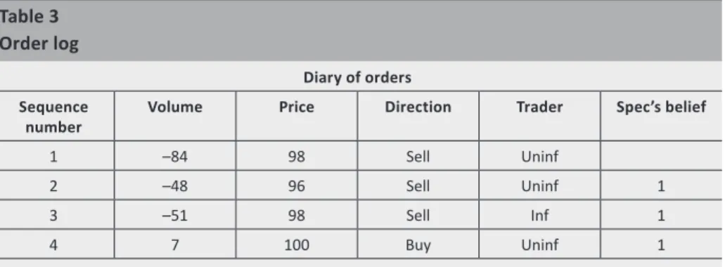
We used two different logs for recording the observations. One of them is the order log.⁶ The relevant subroutine copies all new incoming orders other than 0 into this log; i.e. this log collects all cases where the arriving trader accepted the specialist’s quotation. The log contains the volume of all orders that have a meaningful sign, prices, the buy or sell direction and the fact whether the programme classified the given trader as informed or uninformed. Another subroutine is at work in the last column, which displays the specialist’s belief about whether the given trader was informed or not (Table 3).

Table 3 Order log

Diary of orders Sequence

number Volume Price Direction Trader Spec’s belief

1 –84 98 Sell Uninf

2 –48 96 Sell Uninf 1

3 –51 98 Sell Inf 1

4 7 100 Buy Uninf 1

For understandable reasons, the specialist is not always correct in guessing the trader’s type (as shown by Table 3) as indeed, the specialist can only see whether the given person traded the full depth or not. If yes, the specialist will deem the trader informed (signalled by 1) even though it is also possible that the trader was

6 See Appendix 4

uninformed but by chance, his demanded volume coincided with the quoted depth.

The sum of the numbers contained in this “Spec’s belief” column gives the k value for Proposition (2); i.e. the number of full-depth trades, while the last sequence number of the log at a given moment gives the N value, which denotes the number of all trades completed that far.

The second log is the transaction log,⁷ the first five columns of which are generated by another subroutine integrated into the “Order” subroutine. The next four columns are computed by Excel as shown in Table 4.

The transaction log is used for the purposes of inspecting the results.

1. The commission fee column simply contains the order value (volume^•price) multiplied by 1.5 per cent; the value of the latter parameter can be set as required. Wealth is received as the product of current money and price.

2. For the calculation of money and stock, the direction of the transaction should be taken into account. In the case of a sell order, after the t^th transaction money is computed as follows:

money_t=money_t−1+price_t⋅volume_t+commission fee_t (19) In the case of a buy order, the calculation will be:

money_t=money_t−1−price_t⋅volume_t+commission fee_t (20) 3. For stocks, the calculation is the opposite: if it was a sell order, the stock portfolio

decreases after the t^th transaction:

stock_t=stock_t−1−volume_t (21) Conversely, in the case of a buy order, the portfolio increases:

stock_t=stock_t−1+volume_t (22) Table 4

Transaction log Sequence

number Type Volume Price Spread Commission

fee Money Stock Wealth

1 Buy 84 98 3 123.5 501,699 993 599,013

2 Buy 48 96 4 69.1 497,161 1,041 597,097

3 Buy 51 98 4 75.0 492,238 1,092 599,254

4 Sell 7 100 2 10.5 492,948 1,085 601,448

7 See Appendix 5

5. Evaluation of the results

5.1. Comprehensive statistics

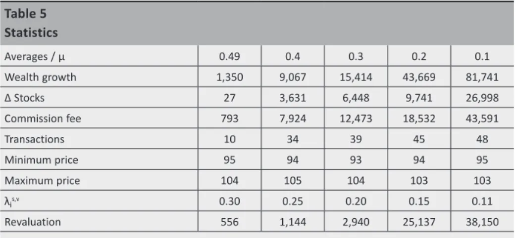
Firstly, we would like to present a statistical table designed to evaluate the simulation as a whole and containing the mean values received for selected µ values. We computed these values with the Monte Carlo method, using the transaction log described in Section 4.3.

Table 5 Statistics

Averages / µ 0.49 0.4 0.3 0.2 0.1

Wealth growth 1,350 9,067 15,414 43,669 81,741

Δ Stocks 27 3,631 6,448 9,741 26,998

Commission fee 793 7,924 12,473 18,532 43,591

Transactions 10 34 39 45 48

Minimum price 95 94 93 94 95

Maximum price 104 105 104 103 103

λi^s,v 0.30 0.25 0.20 0.15 0.11

Revaluation 556 1,144 2,940 25,137 38,150

For each individual case, we ran 20 rounds of the programme where one round means 100 periods, i.e. 100 arriving traders. During the simulation a round takes place as follows:

1) The contents of the order and transaction logs are deleted.

2) The programme generates a new initial order book.

3) The “Order” subroutine runs 100 times (the parameter can be set as needed).

The subroutine calls a trader in each period. The new order is added to the order log, the subroutine books the transaction in the transaction log, and the order book is updated. Obviously, not all traders say yes to the specialist’s offer as it is quite possible that their reservation price is lower/higher than the quoted ask/

bid price. In such cases no transaction takes place; the programme continues to run and the next participant arrives. Meanwhile, the specialist’s quote and the possible final returns on the risky asset change continuously.

4) The results are calculated based on the transaction log.

After having run 20 rounds, the programme computes the mean of the results received at the end of each round, which is included in Table 5.

The means of minimum and maximum prices do not show a significant difference;

apparently, changes in µ did not influence these values unambiguously. Price fluctuations, however, had a greater impact, as will be discussed in Section 5.2.

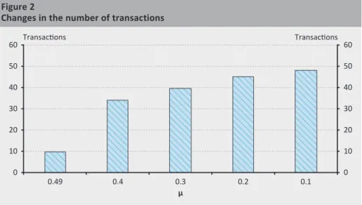
Table 5 also shows the average number of transactions of the 100 periods; in other words, the number of traders who accepted the quote of the specialist. Figure 2 shows an impressive growth rate in line with a declining µ.

The smaller the µ, the smaller the uncertainty about the final payoff of the risky asset and simultaneously, the specialist's expectations about the percentage of informed traders also decrease exponentially (λ_i^s,v indicates the mean value of the specialist’s beliefs calculated from the values at the end of the simulation rounds), even though λ was set to 0.2 throughout the exercise. Table 5 shows that the model behaved best when µ=0.3; that is when it deduced the real value of the specialist’s lambda most accurately on average.

Accordingly, the number of transactions grows in line with the decline in uncertainty for the following reason: the specialist is more likely to know the possible price of the financial product as orders are more likely to come from informed traders, and thus the market price can converge to the fair price with more accuracy during the course of the transactions.

At the beginning of the simulation, the initial earnings of the specialist comprised 500,000 units of money, 1,000 shares, and the commission fee was set at 1.5 per cent. The greater number of transactions combined with the greater certainty about the product’s return may account for the exponential increase in wealth, stocks and commission fees. Revaluation shows how wealth changed once the amount of commission fees was deducted. Table 3 indicates this increment clearly.

Figure 2

Changes in the number of transactions

0 10 20 30 40 50 60

0 10 20 30 40 50

Transactions Transactions 60

0.49 0.4 0.3

μ 0.2 0.1

5.2. Changes in prices

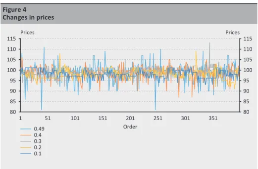
In order to examine the changes in prices and based on the results, changes in logreturns, we ran the code for each µ as many times as to receive nearly 400 observations for all five cases. We calculated their maximum and minimum values and, from the difference of these two, the range and the standard deviation.

Table 6

Minimum and maximum values and range and standard deviation of prices

Price 0.49 0.4 0.3 0.2 0.1

min 81 87 92 91 93

max 111 106 113 109 101

range 30 19 21 18 8

standard deviation 3.95 2.85 2.09 2.20 1.86

Although Table 5 shows that for each µ, the average minimum price is between 93 and 95 and the average maximum price is between 103 and 105 calculated from the values received at the end of the individual rounds, and µ did not appear to exert a clear impact on the prices, Table 6 reveals that µ did have an influence on the prices. This is best demonstrated by the standard deviations of the individual cases. The smaller the uncertainty, the smaller the standard deviation of the prices (with a larger sample size this would be illustrated even more precisely, and the result of 0.3 would fit between 0.4 and 0.2 even better), which is consistent with the findings presented in Section 5.1.

Figure 3

Changes in wealth, stocks and the commission fee

0 10,000 20,000 30,000 40,000 50,000 60,000 70,000 80,000 90,000

0 10,000 20,000 30,000 40,000 50,000 60,000 70,000 80,000 90,000

0.49 0.4 0.3 0.2 0.1

Wealth Δ Shares Commission fee

Figure 4 clearly shows that the smaller the µ value, the smaller the price fluctuation.

5.3. Changes in logreturns

According to the Efficient Market Hypothesis (EMH), market prices fully reflect public information; in other words, all available information is already incorporated into prices and therefore, prices are reliable (Fama 1970). Consequently, prices are shaped only by new information, from which it follows that the daily logreturns are independent and normally distributed (Száz 2009). Therefore, in the next section of our study we examine the extent to which this consequence holds true for the distribution of the logreturns received after the simulation.

We received logreturns from the prices by taking the natural logarithm of the chain indices. Their minimum and maximum values, means and standard deviations are summarised in Table 7.

Table 7

Minimum and maximum values and mean and standard deviation of logreturns

Logreturn 0.49 0.4 0.3 0.2 0.1

min –22.07% –14.92% –11.23% –10.32% –6.19%

max 18.03% 15.91% 10.24% 13.75% 6.19%

mean 0.00% –0.01% –0.01% 0.01% 0.01%

standard deviation 5.38% 3.81% 2.58% 2.14% 1.70%

Figure 4

Changes in prices

80 85 90 95 100 105 110 115

80 85 90 95 100 105 110 115

1 51 101 151 201 251 301 351

Prices Prices

Order 0.49

0.4 0.3 0.2 0.1

We used these values for drawing up the frequency table, taking each individual case separately. Firstly, by using the minimum and maximum values, we prepared an absolute frequency table with 16 class intervals. From this, we calculated actual relative frequencies and then, actual cumulated relative frequencies. After this, we used a built-in Excel function to calculate the values that should be received from a normal distribution with this mean and standard deviation. The numbers received were the values of the cumulative distribution function of the normal distribution, which correspond to the theoretical cumulated relative frequency. Working our way backwards, from this we received the theoretical relative frequencies, and after multiplying these values by the number of observations we received the theoretical absolute frequencies.

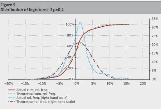
The best result was received when µ=0.4 (Figure 5): this is when the distribution of logreturns most closely approximated the normal distribution, although even then, the probability density function was far more peaked than the normal bell curve.

The cumulative distribution functions are fit to the primary axis and the probability density functions to the secondary.

In Figure 6, we show the distribution of the logreturns received for each of the five µ-s together. This pattern meets our expectations as it shows that the smaller the µ – i.e. the smaller the uncertainty about the ultimate value of the risky product – the more biased the probability density function of the actual logreturns relative to that of the normal return. Accordingly, the more information the specialist has about the asset’s payoff, the more impaired the EMH; namely, that all information

Figure 5

Distribution of logreturns if µ=0.4

0%

5%

10%

15%

20%

25%

30%

35%

0%

20%

40%

60%

80%

100%

–20% –15% –10% –5% 0% 5% 10% 15% 20%

Actual cum. rel. freq.

Theoretical cum. rel. freq.

Actual rel. freq. (right-hand scale) Theoretical rel. freq. (right-hand scale)

available is incorporated into prices and thus, the distribution of the logreturns fits the normal curve less and less. A larger sample size would probably result in an even more spectacular demonstration of the continuous upward bias.

The case where µ=0.49 is apparently more biased compared to the case featuring the 0.4 value. This is probably because in that case µ seldom meets the criteria defined with the inequality included in Proposition (1) and therefore, the programme applies the passive quotation type instead of the active equilibrium model proposed by Caglio − Kavajecz.

6. Summary

The purpose of our study was to write a simulation programme that may allow us to examine the impact of adverse selection on the specialist’s price quotation, the extent to which various levels of uncertainty influence prices and logreturns, and the accuracy to which the specialist can determine the proportion of informed traders on the market based on the transactions.

Based on the simulation, the specialist’s belief about the ratio of informed traders was the most accurate where µ=0.3 on average.

The results showed unambiguously that the number of transactions grows in line with the decline in uncertainty, as the specialist becomes more likely to predict the potential price of the financial product. Parallel to this, both the specialist’s earnings and stock portfolio increase progressively.

Figure 6

Distribution of logreturns for each µ value under review

0%

10%

20%

30%

40%

50%

60%

–20% –15% –10% –5% 0% 5% 10% 15% 20%

0.49 0.1 0.2 0.4 0.3

At the same time, price fluctuation and the standard deviation of logreturns decline continuously, and the consequence of the efficient market theory, namely, that the standard deviation of logreturns follows a normal distribution, becomes more and more biased as the condition that prices reflect public information becomes impaired.

Table 8 sums up these results. Analogously, when the process is reversed: an increase in uncertainty will trigger an opposite change in the other areas.

Table 8

Impact of changes in uncertainty

Uncertainty (µ) decreases

Number of transactions increases

Wealth increases

Stocks increases

Price fluctuation decreases

Standard deviation of logreturns decreases

Fit of logreturns to normal distribution decreases

The results were consistent with our expectations and of course, their precision and clarity would probably improve further with a bigger sample size and repeated runs of the programme.

References

Bagehot, W. (1971): The only game in town. Financial Analyst Journal, 27(2): 12–14. https://

doi.org/10.2469/faj.v27.n2.12

Caglio, C. – Kavajecz, K.A. (2006): A Specialist’s quoted depth as a strategic choice variable:

An application to spread decomposition models. The Journal of Financial Research, 29(3):

367–382. https://doi.org/10.1111/j.1475-6803.2006.00184.x

Copeland, T.E. – Galai, D. (1983): Information Effects on the Bid-Ask Spread. The Journal of Finance, 38(5): 1457–1469. https://doi.org/10.1111/j.1540-6261.1983.tb03834.x Demsetz, H. (1968): The cost of transacting. The Quarterly Journal of Economics, 82(1):

33–53. https://doi.org/10.2307/1882244

Doob, J.L. (1971): What is a martingale? The American Mathematical Monthly, 78(5): 451–

463. https://doi.org/10.2307/2317751

Dupont, D. (2000): Market Making, Prices and Quantity Limits. The Review of Financial Studies, 13(4): 1129–1151. https://doi.org/10.1093/rfs/13.4.1129

Easley, D. – O’Hara, M. (1992): Time and the Process of Security Price Adjustment. The Journal of Finance, 47(2): 577–605. https://doi.org/10.2307/2329116

Fama, E.F. (1970): Efficient capital markets: A review of theory and empirical work. The Journal of Finance, 25(2): 383–417. https://doi.org/10.2307/2325486

Foucault, T. – Pagano, M. – Röell, A. (2013): Market Liquidity. Oxford University Press, New York.

Glosten, L.R. – Milgrom, P.R. (1985): Bid, ask and transaction prices in a specialist market with heterogeneously informed traders. Journal of Financial Economics, 14(1): 71–100. https://

doi.org/10.1016/0304-405X(85)90044-3

Harris, L. (1990a): Statistical Properties of the Roll Serial Covariance Bid/Ask Spread Estimator.

Journal of Finance, 45(2): 579–590. https://doi.org/10.1111/j.1540-6261.1990.tb03704.x Harris, L. (1990b): Liquidity, Trading Rules, and Electronic Trading Systems. New York

University Monograph Series in Finance and Economics, Monograph 1990–4.

Kavajecz, K.A. (1999): A Specialist’s Quoted Depth and the Limit Order Book. The Journal of Finance, 54(2): 747–771. https://doi.org/10.1111/0022-1082.00124

Kavajecz, K.A. – Odders-White, E. R. (2001): An Examination of Changes in Specialists’ Posted Price Schedules. The Review of Financial Studies, 14(3): 681–704. https://doi.org/10.1093/

rfs/14.3.681

Kornis, J. (2017): Árjegyzési stratégiák vizsgálata Monte Carlo szimulációval (Examining price quotation strategies using the Monte Carlo simulation). Thesis, Corvinus University of Budapest.

Kutas, G. – Végh, R. (2005): A Budapesti Likviditási Mérték bevezetéséről (Introduction of the Budapest Liquidity Measure). Közgazdasági Szemle (Hungarian Economic Review), 52(7–8): 686–711.

Kyle, A.S. (1985): Continuous Auctions and Insider Trading. Econometrica, 53(6): 1315–1335.

Lee, C.M.C. – Mucklow, B. – Ready, M.J. (1993): Spreads, Depths and the Impact of Earnings Information: An Intraday Analysis. The Review of Financial Studies, 6(2): 345–374. https://

doi.org/10.1093/rfs/6.2.345

O’Hara, M. (1995): Market Microstructure Theory. Basil Blackwell. Cambridge, MA.

Rock, K. (1989): The Specialist’s Order Book. Working Paper, Harvard University.

Száz, J. (2009): Pénzügyi termékek áralakulása (Price Formation of Financial Products). Jet Set Tipográfiai Műhely Kft. Budapest.

Von Wyss, R. (2004): Measuring and predicting liquidity in the stock market. PhD Dissertation, Universität St. Gallen.

Appendices

The appendices of our paper present the most important subroutines and functions written for the simulation.

Appendix 1: Function of the specialist’s quotation I

As mentioned before, the function combines two methods. If µ fulfils condition (1) – which consists of two inequalities – then the equilibrium values will be consistent with Caglio and Kavajecz (2006). If the inequality is not fulfilled, then the programme jumps to the next commands. The same command is run even when it is not only the second half of the inequality that is unfulfilled, but also the first part of it. At the end of the function, a built-in function rounds up the generated bid and ask prices and volumes to the nearest whole number.

Function specialist(mu, v1, v2, lambdaS, t1, t2, spmax, spmost) Dim Ev, v21, t21

ReDim assumption(1 To 2) ReDim bidask(1 To 4)

Ev = mu * v1 + (1 - mu) * v2 ‘expected value of the asset v21 = v2 - v1

t21 = t2 - t1

assumption(1) = (lambdaS - lambdaS * t2 / t1) / (1 - lambdaS * t2 / t1) assumption(2) = (1 - lambdaS) / (1 - lambdaS * t2 / t1)

If assumption(1) < mu Then ‘condition (1) is fulfilled If mu < assumption(2) Then ‘condition (2) is also fulfilled ‘bid size

beta = 3 / 2 * t2 - 1 / 2 * t2 * (1 + (8 / t2) * (lambdaS / (1 - lambdaS)) * (mu / (1 - mu)) * t21) ^ 0.5

‘bid price

b = 1 / 4 * (3 * Ev + v1) - 1 / 4 * (1 - mu) * v21 * (1 + (8 / t2) * (lambdaS / (1 - lambdaS)) * (mu / (1 - mu)) * t21) ^ 0.5

‘ask size

alpha = 3 / 2 * t1 - 1 / 2 * t1 * (1 - (8 / t1) * (lambdaS / (1 - lambdaS)) * ((1 - mu) / mu) * t21) ^ 0.5

‘ask price

a = 1 / 4 * (3 * Ev + v2) + 1 / 4 * mu * v21 * (1 - (8 / t1) * (lambdaS / (1 - lambdaS)) * ((1 - mu) / mu) * t21) ^ 0.5

Else ‘but condition 2 is not fulfilled

If spmost <= spmax Then ‘if the spread is good For i = 3 To 45

If Cells(i, 12) > 0 Then beta = Cells(i, 12) b = Cells(i, 13) GoTo 51 End If Next i

51 For i = 45 To 3 Step -1 If Cells(i, 14) > 0 Then alpha = -Cells(i, 14) a = Cells(i, 13) GoTo 53 End If Next i Else

‘if the spread is higher than permitted For i = 3 To 45

If Cells(i, 12) > 0 Then beta = 150

b = Cells(i, 13) + 1 GoTo 52

End If Next i 52

For i = 45 To 3 Step -1 If Cells(i, 14) > 0 Then alpha = -150 a = Cells(i, 13) - 1 GoTo 53

End If Next i 53

End If End If

Else ‘even condition 1 is unfulfilled If spmost <= spmax Then ‘if the spread is good For i = 3 To 45

If Cells(i, 12) > 0 Then

beta = Cells(i, 12) b = Cells(i, 13) GoTo 54 End If Next i 54

For i = 45 To 3 Step -1 If Cells(i, 14) > 0 Then alpha = -Cells(i, 14) a = Cells(i, 13) GoTo 56 End If Next i Else

‘if the spread is higher than permitted For i = 3 To 45

If Cells(i, 12) > 0 Then beta = 150

b = Cells(i, 13) + 1 GoTo 55

End If Next i

55 For i = 45 To 3 Step -1 If Cells(i, 14) > 0 Then alpha = -150 a = Cells(i, 13) - 1 GoTo 56

End If Next i 56 End If End If

bidask(1) = Application.Round(beta, 0) bidask(2) = Application.Round(b, 0) bidask(3) = Application.Round(alpha, 0) bidask(4) = Application.Round(a, 0) specialist = bidask

End Function