Non-Linear Exchange Rate Dynamics in Target Zones: A Bumpy Road Towards A Honeymoon

Non-Linear Exchange Rate Dynamics in Target Zones: A Bumpy Road Towards A Honeymoon

Jesús Crespo-Cuaresma Balázs Égert

Ronald MacDonald

May 12, 2005

Abstract

This study investigates exchange rate movements in the Exchange Rate Mechanism (ERM) of the European Monetary System (EMS) and in the Exchange Rate Mechanism II (ERM-II). On the basis of the variant of the target zone model proposed by Bartolini and Prati (1999) and Bessec (2003), we set up a three-regime self-exciting threshold autoregressive model (SETAR) with a non-stationary central band and explicit mod- elling of the conditional variance. This modelling framework is employed to model daily DM-based and median currency-based bilateral exchange rates of countries participating in the original ERM and also for exchange rates of the Czech Republic, Hungary and Slovakia from 1999 to 2004.

Our results con…rm the presence of strong non-linearities and asymme- tries in the ERM period, which, however, seem to di¤er across countries and diminish during the last stage of the run-up to the euro. Important non-linear adjustments are also detected for Denmark in ERM-2 and for our group of four CEE economies.

Keywords: target zone, ERM, non-linearity, SETAR.

JEL:F31, G15, O10

University of Vienna, E-mail: jesus.crespo-cuaresma@univie.ac.at

yCorresponding author; Oesterreichische Nationalbank; MODEM, University of Paris X- Nanterre and William Davidson Institute. E-mail: balazs.egert@oenb.at and begert@u- paris10.fr

zUniversity of Glasgow and CESIfo, E-mail: r.macdonald@socsi.gla.ac.uk

xThe authors would like to thank Marie Bessec, Harald Grech, Sylvia Kaufmann, Peter Mooslechner, Thomas Reininger and Timo Teräsvirta for helpful comments and suggestions.

The paper also bene…ted from comments from participants at an internal seminar at the Oesterreichische Nationalbank. We are grateful to André Verbanck from the European Com- mission (DG ECFIN) for providing us with the data series for the median currency. The opinions expressed in this paper are those of the authors and do not necessarily re‡ect the views of the Oesterreichische Nationalbank or the European System of Central banks (ESCB).

1 Introduction

The seminal paper of Krugman (1991) focused on explaining the exchange rate behaviour of a currency with a central parity rate and upper and lower exchange rate bands, the so called target zone model. The existence of the Exchange Rate Mechanism (ERM) of the European Monetary System (EMS) provided researchers with an ideal opportunity to test the target zone model because it provided ample data for empirical analysis. Since the early 1990s, numerous papers have been written on the period preceding the ERM crisis of 1993,¹ while the period in the run-up to the euro has received less attention.² How- ever, further analysis of the post-1993 experience would appear to be fruitful for, at least, two reasons. First, Flood, Rose and Mathieson (1990) and Rose and Svensson (1995) reported only limited non-linearity in the period prior to 1993. However, the widening of the ‡uctuation bands from 2:25% to 15%

in the post-1993 period may have introduced additional non-linear behaviour into exchange rate behaviour. Second, the recent enlargement of the European Union to 25 countries implies that the New Member States would participate, at some point in time, in an ERM-2 arrangement, prior to their adoption of the euro. For them, there may be useful information contained in the behaviour of ERM currencies prior to the introduction of the euro in 1999.

The empirical literature on target zones su¤ers from a number of problems.

First, most studies use monthly or weekly frequencies, which may ‘aggregate out’

the true dynamics of the exchange rate process. Second, the frequent jumps in the central parity in the ERM are not adequately accounted for in the pre-1993 period. Finally, either the mean³ or variance equation⁴ is investigated in a more sophisticated way instead of modelling them jointly.

The aim of this study is to shed additional light on exchange rate behaviour in ERM, ERM-2 and CEE countries. Our modelling framework is based on the target zone models set out in Bartolini and Prati (1999) and Bessec (2003).

These models predict the presence of soft bands within the o¢ cially announced large bands. More speci…cally, these models assume that the monetary author- ities do not intervene in the proximity of the central parity. In this area, the exchange rate behaves like a random walk. However, the monetary authorities take policy action when the exchange rate is about to leave this corridor. Thus, the exchange rate exhibits mean reversion towards the soft band. However, it should be noted that, in reality, such band mean reversion could be the outcome of a number of factors, such as direct and indirect central bank interventions, moral persuasion, communication with the markets, stabilisation of market ex- pectations, in the face of increased credibility of the monetary authorities, or because of an increased stability of the underlying fundamentals. This type of

1Examples are Anthony and MacDonald (1998), Bessec (2003), Bekaert and Gray (1998), Chung and Tauchen (2001), Rose and Svensson (1995).

2See, for example, Anthony and MacDonald (1999), Bessec (2003) and Brandner and Grech (2002).

3For example, Bessec (2003) models the mean equation using a SETAR model.

4Brandner and Grech (2002) use a simple AR process for the mean equation and use di¤erent GARCHG models for the variance equation.

behaviour is best captured by a three-regime SETAR model in which we model conditional variance by means of a GARCH(1,1). The application of this model for daily data from the post-1993 ERM and ERM-2 does not only indicate the presence of a three-regime threshold model but also considerable asymmetries for the detected upper and lower bounds that delimit the soft band within the announced target zone.

The remainder of the paper is structured as follows: Section 2 overviews the target zone literature and summarizes the principal features of this class of models. Section 3 sets out the econometric framework. Section 4 provides the description and a …rst analysis of the data used in the paper. Section 5 analyses the empirical results and Section 6 provides some concluding remarks.

2 Target Zone Models

2.1 The Krugman Model: Perfect Credibility with Mar- ginal Interventions

The baseline target zone model presented in Krugman (1991) is based on a continuous-time representation of the ‡exible-price monetary model in which the exchange rate (e) is assumed to be a linear function of a set of fundamental variables (f) and the expected change of the exchange rate (E(de)=dt):⁵

e=f+ E(de)=dt (1)

The fundamentals explicitly considered by Krugman (1991) are money sup- ply and velocity. Money supply is controlled by the monetary authorities, whereas velocity is exogenous. First, it is assumed that the announced ‡uc- tuation band around the central parity is perceived by market participants as fully credible. Perfect credibility implies that neither the ‡uctuation bands nor the central parity would be altered and that the exchange rate would remain inside the ‡uctuation band. Second, it is assumed that the monetary authorities only intervene when the exchange rate hits the upper or lower bound of the of-

…cially announced ‡uctuation band. The implication of the second assumption is that the exchange rate behaves within the ‡uctuation band as under a free

‡oat. Because velocity is assumed to follow a standard Wiener, or Brownian motion, process without drift⁶ and because the money supply is considered con- stant under a free ‡oat (with the expected change in the exchange rate being equal to zero) the nominal exchange rate also follows a Brownian motion and depends proportionally on the fundamentals, i.e. velocity.

Under the assumptions sketched out above, the general solution of the model becomes the following:

e=f+A exp( f) +B exp( f) (2)

where A and B are constants, =q

2= ²_f, fis the standard deviation of the fundamentals and denotes the elasticity of real money supply to the interest rate in the structural form of the monetary model. Equation (2) is composed of a linear and a non-linear part. The linear part, f, represents the solution for a free-‡oat. However, the main results of the model, which came to be known as the honeymoon e¤ ect and smooth pasting are re‡ected in the non- linear part, A exp( f) +B exp( f). The honeymoon e¤ect refers to the phenomenon that if the exchange rate is close to the weaker (stronger) edge of the band, the probability increases that the exchange rate will hit the edge,

5Recall that under the assumption of uncovered interest parity, the standard discrete-time form of the monetary model can be written as: et =mt m_t (yt y_t) + e^e_t+1 with

; > 0, m and m denoting domestic and foreign money supply, y and y standing for domestic and foreign output and e^e_t+1 representing the expected change in the nominal exchange rate in period t for period t+1.

6This is indeed the continuous-time representation of a random walk.

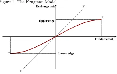
which automatically leads to interventions by the monetary authorities. As a consequence, the probability that the exchange rate appreciates (depreciates) is higher than the probability that it depreciates (appreciates). This is depicted in Figure 1. From this it follows that the exchange rate will be less depreciated (appreciated) given by the line TT than the level that would be given by the fundamentals alone (linear component of equation (2)) under a free ‡oat (45- degree line FF). Thus, this type of target zone model stabilises the exchange rate relative to its fundamentals within the ‡uctuation band. Smooth pasting refers to the phenomenon that the path of the exchange rate smoothes out on its way to the boundaries of the band and its slope becomes zero when it eventually hits the edge.

Figure 1. The Krugman Model

Exchange rate F

T Upper edge

Fundamental

T Lower edge

F

A crucial implication of the baseline Krugman model is that the exchange rate will spend more time close to the boundaries than inside the target zone.

Consequently, the distribution of the exchange rate will be U-shaped between the upper and lower bounds. Lundbergh and Teräsvirta (2003) demonstrate for the case of Norway from 1986 to 1988 that provided the two main assumptions are satis…ed, i.e. the target zone is perfectly credible and the monetary authori- ties intervene only at the edges of the target zone, the Krugman model is able to describe surprisingly well the exchange rate behaviour in Norway in the period considered.

2.2 Extensions of the Krugman Model

Target zone exchange rate regimes may not be fully credible because the central parity may be realigned and the ‡uctuation bands widened. If realignment causes a shift in the band which does not overlap with the previous band, the exchange rate will jump. This may or may not be the case if there is

7For a very detailed presentation of the extensions, see e.g. Svensson (1992) and Kempa and Nelles (1999).

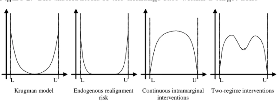
an overlap between the old and new bands. Numerous realignments took place, for instance, within the ERM⁸ and also in transition countries such as Poland and Hungary . Given such discontinuities, a number of attempts have been made to relax the assumption of perfect credibility and allow for jumps in the central parity. Table 1 summarises the main features of the di¤erent extensions and Figure 2 gives the distribution of the exchange rate within the o¢ cially announced ‡uctuation bands.

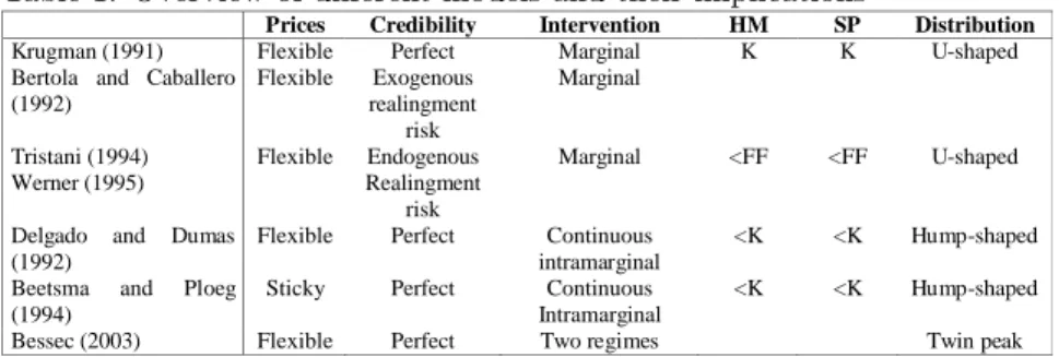
Table 1. Overview of di¤erent models and their implications

Prices Credibility Intervention HM SP Distribution

Krugman (1991) Flexible Perfect Marginal K K U-shaped

Bertola and Caballero (1992)

Flexible Exogenous realingment

risk

Marginal

Tristani (1994) Werner (1995)

Flexible Endogenous Realingment

risk

Marginal <FF <FF U-shaped

Delgado and Dumas (1992)

Flexible Perfect Continuous intramarginal

<K <K Hump-shaped Beetsma and Ploeg

(1994)

Sticky Perfect Continuous Intramarginal

<K <K Hump-shaped

Bessec (2003) Flexible Perfect Two regimes Twin peak

Notes: HM= honeymoon e¤ect, K denotes the honeymoon e¤ect and smooth- pasting under the Krugman solution. <K (<FF) signals the respective e¤ects being smaller than in the Krugman model (free ‡oat).

Figure 2. The distribution of the exchange rate within a target zone

L U L U L U L U Krugman model Endogenous realignment

risk

Continuous intramarginal interventions

Two-regime interventions

2.2.1 Imperfect credibility with exogenous realignment risk

Bertola and Caballero (1992) allow for exogenous realignment risk. The central parity (c), set to zero in the Krugman model is now considered to become part of the aggregate fundamental variable: f =v +cwherevis a stochastic term and is the fundamental. The monetary authorities will defend the currency with probability (1-p) when it reaches the edges of the band and will proceed

8Note that no realignment took place for Greece and Denmark in the ERM-2.

with realignment of the central parity with probability p. Realignment is as- sumed to be re‡ected in a shift of the band. The general solution of the model is now as follows:

e=f +A exp( (f c)) +B exp( (f c)) (3) The model with exogenous realignment risk implies that under certain cir- cumstances (p 0:5), both the honeymoon e¤ect and smooth pasting disappear.

2.2.2 Imperfect credibility with endogenous realignment risk Clearly, the fact that realignment risk is modelled as exogenous and that realign- ment only takes place when the exchange rate is at the edges of the band may be too restrictive and need not apply in reality. Tristani (1994) and Werner (1995) set out to model realignment risk as endogenous by assuming that the probabil- ity of realignment is a positive function of how far the exchange rate is located from the central parity - the larger the distance, the higher the probability of realignment. The general solution of their model is given by:

e c= (f c) (1 + p

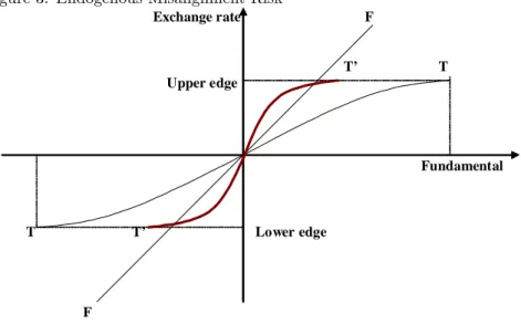
w ) +A exp( (f c)) +B exp( (f c)) (4) where ; pand w stand for the size of realignment, the probability of a realignment (which is a function of the deviation from the central parity) and the width of the target zone, respectively. Figure 3 shows that a result of the model is that the S curve becomes steeper (line T’T’) when compared to the S curve obtained from the Krugman model (Figure 1.). This in turn implies an even stronger U-shaped distribution of the exchange rate within the band.

Figure 3. Endogenous Misalignment Risk

Exchange rate F

T’ T Upper edge

Fundamental

T T’ Lower edge

F

2.2.3 Perfect credibility with intramarginal interventions

The second main assumption of the Krugman model could fail because the monetary authorities may wish to intervene within the band (i.e intra marginal intervention) and not just in case the exchange rate hits the upper or lower edges of the band (marginal intervention). Mastropasqua et al. (1988) and Delgado and Dumas (1992) argue that about 85% to 90% of total interventions took the form of intramarginal intervention in the ERM before the crises in 1992 and 1993. Regarding the post-crisis period, the exchange rate never hit the upper or lower bound of any of the participating countries, which implies that all interventions were necessarily intramarginal.⁹ As a result, it comes as no surprise that the distribution of the exchange rate is usually found to be hump-shaped for currencies participating in ERM and ERM-2, suggesting that the exchange rate spends most of the time in the middle of the band rather than close to the boundaries of the target zone.

Considerable e¤ort has been made to build target zone models that are able to account for intramarginal interventions. For example, Delgado and Dumas (1992) modify the Krugman model so as to account for intramarginal interventions, which are assumed to take place continuously inside the target zone if the exchange rate deviates from the central parity. The solution provided by Delgado and Dumas (1992) is:

e=f + pf0

1 + p +AM( 1 2 p;1

2;p(f0 f)²

2v

)+BM(1 + p 2 p ;3

2;p(f0 f)²

2v

)

pp(f0 f)

v

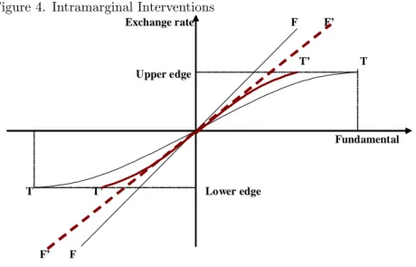
(5) where M is the hypergeometric function and f₀ being the fundamental’s value when the exchange rate is equal to the central parity. Figure 4 shows the main result of the model: although the honeymoon e¤ect diminishes con- siderably (line T’T’) when compared to the honeymoon e¤ect under perfect credibility and marginal intervention, the exchange rate is nonetheless still less volatile than under free-‡oat.¹⁰ Similarly, smooth pasting is also substantially reduced in this set up because market agents know that monetary authorities have already intervened. If A and B are set to zero, the Delgado and Dumas solution collapses toe=^f+₁₊^pf_p⁰, which happens to be the case of managed ‡oat- ing without …xed boundaries. In such a setting, all interventions would qualify as intramarginal. The solution shows that the exchange rate is stabilised com- pared to the free-‡oat position and interventions induce a mean reversion of the exchange rate towards the central parity (line F’F’). Put di¤erently, even in the absence of a formal target zone-type of exchange rate arrangement, central bank interventions can stabilise the exchange rate relative to the case of a free-‡oat.

9Brandner and Grech (2002) provide some summary statistics on the intervention activity of the participating countries’ central banks after 1993.

1 0Note that this is not necessarily the case in a multilateral target zone with intramarginal interventions. For example, Serrat (2000) shows that in such a setting , exchange rate volatility can be larger than under a free ‡oat.

Figure 4. Intramarginal Interventions

Exchange rate F F’

T’ T

Upper edge

Fundamental

T T’ Lower edge

F’ F

2.2.4 Sticky prices with intramarginal interventions

A major drawback of the models presented above is that they are based, without exception, on the ‡exible-price monetary model, which assumes that purchasing power parity (PPP) holds continuously. However, it is a well-established fact that PPP does not hold continuously¹¹, and therefore some kind of rigidities should be introduced into the modelling framework. Following the example of the Dornbusch overshooting model, Miller and Weller (1991) introduce sticky prices into the Krugman model. In addition to sticky prices, Beetsma and Ploeg (1994) complete the model with intramarginal interventions and show that sticky prices coupled with intramarginal interventions leads to a hump- shaped distribution of the exchange rate within the target zone.

2.2.5 Uno¢ cial bands within the target zone

Bessec (2003) proposes that it is unlikely that monetary authorities would be willing to intervene continuously, independently of the distance of the exchange rate from the central parity. Instead, she argues that it is more likely that monetary authorities do not intervene in the immediate neighbourhood of the central parity and allow the exchange rate to ‡uctuate in a given corridor around the central parity. Only if the exchange rate exits this corridor do the monetary authorities step in to intervene. This kind of regime can be described by the combination of the Krugman model and the Delgado and Dumas model. For example, consider and , which denote, respectively, the upper and lower bounds within the band beyond which the monetary authorities intervene in order to bring back the exchange rate to the central parity. The solution is thus a

1 1See e.g. Rogo¤ (1996) and MacDonald (1995,2004).

combination of the free-‡oat Krugman solution, ifeL e eU, and the Delgado and Dumas solution in case the exchange rate is below the lower bound (e < eL) or above the upper bound (e > e_U)¹²:

e= 8<

:

DELGADO DU M AS_solution if e > e_U KRU GM AN_f ree f loat_solution if e_L e e_U

DELGADO DU M AS_solution if e < e_L

(6)

Notice that the upper and lower regimes need not have equal parameters because the monetary authorities may have asymmetric preferences. Table 1 hereafter summarises the main features of the di¤erent models and the corre- sponding exchange rate distributions are plotted in Figure 2.

Although the theoretical model suggests that it is only intramarginal in- terventions by the monetary authorities that create a band of inaction, it is worth noting that, in practice, a large number of other factors may also be responsible. Such factors are the ability of the monetary authority to stabilise the national currency by other policy actions. Second, moral persuasion and appropriate communication towards the markets are also likely to in‡uence the exchange rate. More particularly, market expectations and the credibility of the monetary authorities are likely to play a big role. If the monetary authorities are credible, it may su¢ ce to intervene in very small amounts in the market to persuade agents that the exchange rate will remain stable. Or, even better, the possibility of market intervention and a well established track record of the monetary authorities may bring about relative exchange rate stability. Finally, expectations may also be stabilised because of fundamentals becoming increas- ingly stable, or because of expected future developments of the fundamentals.

This kind of e¤ect may have played a special role in the run-up to the euro in the late 1990s, when the markets expected a high degree of macroeconomic convergence to occur across countries. Therefore, the band of inaction could be viewed as a band where the exchange rate dynamics resemble a random walk process whereas outside the band, the above factors can result in the exchange rate mean reverting. In the remainder of the paper, when using the expression

‘band of inaction’, we have this broader interpretation in mind.

1 2Bartolini and Prati (1999) develop a di¤erent model that may be able to capture such behaviour. In particular, they argue that there is a narrow, uno¢ cial band within the o¢ cially announced band. The narrow band is soft in that its boundaries are not only not publicly announced but also they change given that a moving average rule based on past values of the exchange rate is assumed. This set up is indeed very close to reality given that the European Monetary Institute and the ECB evaluated the criterion on exchange rate stability on the basis of a 10-day moving average.

3 Econometric Issues: The SETAR-GARCH model

In this section, we propose a simple non-linear time series model with local non- stationary behaviour but overall ergodic characteristics, which is a discrete-time representation of the mixed-solution model proposed by Bessec (2003). The model aims to detect the non-stationary behaviour of the exchange rate within an o¢ cial band ( ₂, ₁), when it stays within the band of inaction around the o¢ cially announced central parity, while allowing for global mean rever- sion towards the band of inaction contemplated by the monetary authorities.

The speci…cation we propose is a simple three-regime self-exciting threshold au- toregressive (SETAR) model with a central band in which the variable behaves like a unit root process. The errors in the speci…cation have a simple GARCH (1,1) structure in order to account for the time-varying variance and volatility clustering observed in the data.

The speci…cation of the model is the following,

y_t= 8>

>>

>>

><

>>

>>

>>

:

0+ 1yt 1+ PK

k=1 k yt k+ t ifyt 1 1 0+

PK k=1

k yt k+ t if ₁ yt 1 2

0+ ₂y_{t 1}+ PK k=1

k y_{t k}+ _t if ₂ y_{t 1}

(7)

where the error term, "t, is assumed to follow a GARCH (1,1) process,

tjItN(0; t) and,

2

t = + ²_{t 1}+ ²_{t 1} (8)

where It refers to the information set available in period t. Notice that if

i 2 ( 1;0); i = 1;2; for suitable values of ₀, and ₀, y_t will present overall mean reverting features to the band ( ₁, ₂), which is assumed to be contained in the o¢ cial band ( ₂, ₁). Inside the band, however, the variable behaves as a unit root process with GARCH errors. A homoskedastic version of this model is used in Bessec (2003) to assess the dynamics of the exchange rate of selected countries within ERM.

We intend estimating the model given by (7) - (8) in the following way. For a given series yt , the model is estimated setting the values of ₁ and ₂ to actual realizations ofytin the sample (say starting with the tenth and ninetieth percentile of the empirical distribution of yt). The process is repeated for all combinations of ₁and ₂ corresponding to realized values (after ensuring that a minimal percentage of the observations falls in the central band) and the pair (y1; y2) corresponding to the model with a minimal sum of squared residuals is chosen as the estimator of ( ₁, ₂). Given the estimates of the threshold values,

which are constant over time, and which delimit the band, the estimation of the full model is straightforward using maximum likelihood methods.

In our analysis, we obtain the estimates for the thresholds that de…ne the band using a grid search over the realized values of yt after trimming 10% in the extremes of the empirical distribution of yt. The grid search was carried out at 5% steps, ensuring that at least 20% of the observations fall in the nonstationary regime de…ned by the band.

An important issue that needs to be taken into account explicitly is how to test the signi…cance of the the simple unit root against non-linear model.

Due to the fact that the threshold parameters ₁ and ₂ are not identi…ed under the null hypothesis of a linear unit root process with GARCH errors, the usual likelihood ratio test statistic for testing this hypothesis against the alternative of a SETAR model such as (7)-(8) does not have a standard limiting distribution (for literature on this problem, see Andrews and Ploberger, 1994, Hansen, 1996, 2000; Caner and Hansen, 2001, consider the problem when the underlying stochastic process has a unit root). We therefore intend carrying out the test using a bootstrap procedure in the spirit of Hansen (2000) and Caner and Hansen (2001). Let T be the sample size. First, we compute the standard likelihood ratio (LR) test statistic,

LR= 2(logL_{T AR} logL_{U R});

whereL_{T AR}R is the likelihood of the model given by (7)-(8) andL_{U R} is the likelihood of the linear unit root model given by

yt= 0+ XK k=1

k yt k+ t; (9)

where the error term is assumed to follow a GARCH (1,1) process such as the one given in (8). With the estimated parameters of model (9) (including the estimated GARCH parameters), we simulate T observations ofytunder the null of linearity. A linear unit root model and a SETAR model are estimated using these simulated data, and the likelihood ratio test statistic,LR^s_n, is computed.¹³ This procedure is repeated N times and the bootstrap p-value for the null of a unit root process against the alternative of a SETAR model such as (7)-(8) is given by

p_LR= XN n=1

I(LR > LR^S_n)=N

whereI(:)is the indicator function that takes the value of 1 if the argument is true and zero otherwise. That is, the p-value corresponds to the proportion of simulated likelihood ratio test statistics that exceed the value of the test

1 3Given that it is not ensured that the replicated data will actually cross the estimated thresholds, the SETAR models for the simulated data are estimated setting the thresholds at the quantiles of the replicated series corresponding to the estimated thresholds obtained with the actual data.

statistic computed with the actual data.¹⁴ The bootstrap test was carried out using N=500 replications.

4 Data Issues

4.1 Data Description

The dataset contains average daily deviations of nominal exchange rates vis-à-vis the prevailing central parity.¹⁵ The currencies considered are of countries which participated in the system: Austria, Belgium, Denmark, Finland, France, Ger- many, Ireland, Italy, the Netherlands, Portugal and Spain. Although the ECU was the o¢ cial currency of the ERM, it is widely acknowledged that ERM was centred around the German mark. Therefore, we use exchange rate series vis-à- vis the German mark and these data were obtained from the Bundesbank.¹⁶ In its convergence report of 1998, in the run-up to the euro, the European Commis- sion used the median currency¹⁷ as the benchmark currency for the assessment of the criterion on exchange rate stability. To our knowledge, the median cur- rency has not been used in any previous study aimed at testing target zone models. Thus, we also look at the deviations vis-à-vis the median currency.¹⁸ For the German mark, the time period is the post-1993 crisis period: it begins in September, 1 1993 and ends in February, 28 1998. Although Austria o¢ - cially entered the ERM after its entry to the EU in 1995, the period from 1993 is investigated for this country because it maintained a tight peg with respect to the German mark for this period.¹⁹ Using the extended data for Austria allows us to investigate whether or not the ERM entry provoked a change in exchange rate behaviour. The series are shorter for Finland and Italy, which joined/re-entered ERM, respectively, on October 15 and November 25, 1996.

1 4Notice that the bootstrap test used is a simple example of the non-pivotal bootstrap testing procedures described in Pesaran and Weeks (2001) for non-nested model testing.

1 5Notice that the central parity of the Spanish and the Portuguese currencies were devalued vis-à-vis the German mark on March 6, 1995 by 7% and 3.5%, respectively. That is, the deviations from the central parity are obtained using the central parity prevailing prior to March 6, 1995 and then the devalued central parity from March 6, 1995 onwards. The Irish pound was revalued by 6% on March 16, 1998. This realignment is, however, outside the period investigated in this paper.

1 6See appendix for Datastream codes

1 7“(. . . ) median currency is (the currency) which has an equal number of currencies above and below it within the grid at the o¢ cial ecu …xing on any given day ”(European Commission, 1998, p. 123). In more practical terms, for each participating country, the deviation of the bilateral exchange rate against the ECU from its o¢ cial ECU central parity is determined.

Subsequently, the countries are ranked and the 6th out of the 11 participating currencies is chosen in the ranking. It should be noted that the median currency is chosen on a daily basis, implying that the currency chosen as the median currency could have changed day-by-day.

1 8In addition to the ecu, the German mark and the median currency, three other benchmarks could be, in theory used: (a) the strongest currency of the system, (b) bilateral exchange rates with no benchmark currency and (c) the synthetic euro.

1 9As a matter of fact, Austria had a pegged exchange rate regime vis-à-vis the German mark since the late 1970s. Austria entered the ERM at the …xed peg exchange rate regime it unilaterally maintained beforehand.

For the median currency²⁰, the series runs from March 1, 1996 to February 28, 1998.

For ERM-2, only Denmark is considered and deviations vis-à-vis the central parity against the euro are taken for the period January 4, 1999 to April 28, 2004.²¹ The source of the data are the ECB.²²

Finally, we also analyse the exchange rate behaviour of four CEECs. The exchange rate against the euro is studied for the Czech Republic, Hungary, Poland and Slovakia. For the Czech Republic and Slovakia, the period starts in January 1, 1999 when the euro was introduced. For these two currencies, the deviation against the period average is used because they have been having managed ‡oating. The period begins on March 1, 2000 (close to the outset of free ‡oating, April 12, 2000) for Poland and on May 4, 2001 (the widening of the bands to +/-15%) for Hungary. On June 4, 2003, the central parity was devalued by some 2.26%. As in the case of Portugal and Spain, the deviations vis-à-vis the pre- and the post-devaluation parities are determined. For all four countries, the sample runs to April 28, 2004. Data are drawn from the ECB for the Czech Republic and Poland, from the National Bank of Hungary for Hungary and from Datastream for Slovakia.

4.2 A Preliminary Analysis of the Data

The distribution of the exchange rate within the target zone are estimated using the Epanechnikov kernel density function for 1993 to 1998 (and 1996 to 1998 for Finland and Ireland) vis-à-vis the German mark, for 1996 to 1998 for the median currency and for 1999 to 2004 for the euro. Figures reported in Appendix 2 reveal two important features of the data.

First, a considerable part of the distributions exhibit a double-hump shape.

This is especially the case for the Austrian Schilling, the Danish koruna, the Dutch Gulder, the French frank, the Irish pound and the Portuguese escudo vis- à-vis the deutschemark. With the exception of the Spanish peseta and the Dutch gulder, all currencies have a hump shaped distribution vis-à-vis the median currency.

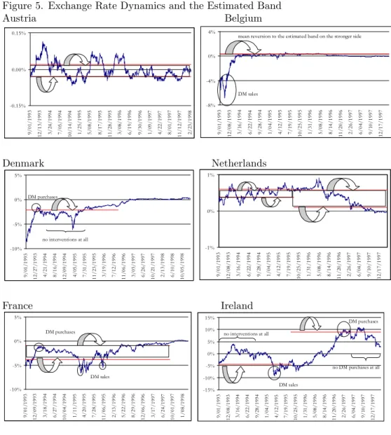
Brandner and Grech (2002)²³ report kernel density estimations for DM pur- chases and sales for 6 countries, namely Belgium, Denmark, Spain, France, Ireland and Portugal. Although the period investigated includes some of the turmoil in August 1993,²⁴ their graphs match remarkably well with our kernel estimates reported in the Appendix for the period from 1993 to 1998. For Bel- gium, they show increase DM sales at the central parity whereas DM purchases occurred at about 0.2% -0.3% in the stronger side of the ‡uctuation band. For

2 0We are grateful to André Verbanck from the European Commission (DG ECFIN) for providing us with these data series.

2 1Greece is excluded because of its ephemeral stay in ERM and ERM-2.

2 2See appendix for Datastream code.

2 3Brandner and Grech (2002), p. 23.

2 4Their sample covers August 2, 1993 to April 30, 1998 while our period spans from Sep- tember 1, 1993 to February 28, 1998.

Denmark, the monetary authorities proceeded with increased DM purchases at 2% from the central parity in the weaker side and sold DM at the central parity.

For France, DM purchases and sales are reported to take place respectively at about 5% and 1% away from the parity on the weaker side. Regarding Ireland, the monetary authorities reportedly sold DM at 5% from the parity on the weaker side and bought DM at 10% from the parity on the stronger side. For Portugal, the interventions at about 4% from the central parity on the weaker side and at 2% from the parity on the stronger side are also broadly in line with exchange rate developments. As for Spain, DM sales are found to occur mostly at 10% from the central parity on the weaker side. A reason for this …nding is that Brander and Grech (2002) start the period in August 1993 during the crisis during.

For the series against the euro, a marked twin peaked distribution is to be observed for the Czech koruna, and to a lesser extent for the Danish and Slovak currencies. This provides us with some preliminary evidence on the presence of non-linearity of the type described by the SETAR model.

The second characteristic of the data is the asymmetric distribution. For the ERM, a large part of the distribution of the Austrian, Danish, French and Portuguese currencies is located on the weaker side of the band. By contrast, the exchange rate was most often on the stronger side of the band for Denmark, Finland and the Netherlands. This holds true, in particular, for the end of the period under study. Regarding the euro series, both countries with formal target zone arrangements, namely Denmark and Hungary, had their currencies predominantly on the stronger side of the band.

5 Empirical results

The SETAR – GARCH(1,1) model described earlier was applied …rst to the exchange rate series vis-à-vis the German mark, for countries participating in ERM. We …rst took the whole post-1993 (after the ERM crisis) until the an- nouncement of the …nal conversion rates in early 1998. Then, the estimations were repeated by decreasing the period by one year in each step until the begin- ning of the reference period taken for the convergence report of the European Commission and the European Monetary Institute is reached.²⁵ Subsequently, the period was shortened by yearly steps, while maintaining the starting date

…xed.²⁶ Finally, the two subperiods determined by the devaluation of the central parity are analysed for Portugal and Spain.²⁷

From the results reported in Table 2a and Table 2b, a number of interesting points emerge. First, the analysis of the estimated upper and lower bounds of the band of inaction shows that there are two groups of countries. The …rst group consists of countries which have very narrow bands for the entire period.

For instance, for the whole period, the absolute bandwidth is 0.05% for Austria, 0.35% for Belgium and 0.15% for the Netherlands.²⁸ The scale of these ranges remains largely unchanged for the subperiods. This is not surprising given the fact that these countries shadowed very narrowly the monetary policy of the Bundesbank and sought to stabilise their currencies relative to the German mark accordingly. The results for Austria deserve special attention. Notwithstanding the fact that Austria formally joined the ERM only in 1995, the estimated upper and lower bounds are very stable over time lending, supporting the proposition that exchange rate behaviour was not a¤ected by Austria’s entry into the ERM.

The second group, comprising the rest of the countries has considerably larger bands. The absolute width of the estimated band was 3.66% for Portugal, 1.28% for France, 3.46% for Denmark, about 4% for Spain and roughly 10% for Ireland for the period from 1993 to 1998. With the exception of Ireland, the estimated bandwidth decreases towards the end of the period: below 1% for Denmark, France and Spain, and close to 2% for Portugal. For Ireland, the estimated bandwidth rises from about 4% from 1993 to 1995 to nearly 8% from 1993 to 1997 and then drops to 2% at the end of the period (1996 to 1998).

Note that Italy and Finland, which entered ERM only in 1996, had bandwidths comparable to that in Belgium and the Netherlands.²⁹

2 5The following three periods were considered: September 1, 1994 to February 28, 1998;

September 1, 1995 to February 28, 1998; March 1, 1996 to February 28, 1998.

2 6The following three periods were considered: September 1, 1993 to September 1, 1997;

September 1, 1993 to September 1, 1996; September 1, 1993 to September 1, 1995.

2 7September 1, 1993 to March 5, 1995 and March 6, 1995 to February 28, 1998.

2 8Notice that the estimation method ensures that at least 20% of the observations fall in the band of inaction.

2 9Our results can be directly compared with those reported in Bessec (2003), who uses monthly data for the Belgian, Danish, French, Irish and Dutch currencies against the German mark. Bessec (2003) estimated a time-varying threshold model for the period from 1979 to 1998 with the threshold changing in 1993 when the ‡uctuation band widened. The comparison of the threshold obtained for the post-1993 shows that our method for searching the thresh- olds, coupled with the use of daily data, gives more precise threshold values. Although the

The second observation regards the position of the estimated band of inaction relative to the o¢ cially announced central parity. Regarding the narrow-band countries, the estimated e¤ective ‡uctuation band is mostly located symmetri- cally from the central parity for Austria, and mainly on the stronger side for Belgium. In the Netherlands, the whole band is always located on the stronger side. Note also that the Italian and Finnish currencies are also found to be situated on the stronger side. For the second group of countries, we note that the boundaries of the estimated exchange rate bands are mostly located on the weaker side of the o¢ cial target zone for Denmark and France. For both countries, the narrowing down of the band manifested itself with the estimated weaker threshold moving closer to the central parity. Although the Portuguese escudo was located on the weaker side at the beginning of the period, the esti- mated band shifted entirely to the stronger side by the last period. For Ireland, Portugal and Spain, the estimated band was on the weaker side from the o¢ cial parity and moved to the stronger side of the o¢ cial ‡uctuation band by the end of the period.³⁰

Third, the estimated autoregressive terms ( upper; _lower), indicating mean reversion to the upper and lower edges ( _upper; _lower), have in the majority of cases the expected negative sign, but they are not statistically signi…cant in a number of cases. Generally, they are more signi…cant for the entire period and then become less so towards the end of the period. However, a more detailed examination of the results indicates considerable heterogeneity across countries.

For Austria, the mean reversion to the band detected for the whole period seems to be unstable because the estimated coe¢ cients are systematically insigni…cant for the sub-periods. Similarly, no signi…cant band mean reversion could be found for Italy.

For the Netherlands and Spain, both coe¢ cients are negative and signi…cant for most of the sub-periods. With regard to Spain, two di¤erent regimes are hidden behind the band mean reversion behaviour detected for the whole period if the time of the devaluation of the central parity is considered as the dividing line for the two sub-periods. The estimated band is situated from 4.04% to 8.34%

away from the o¢ cial central parity on the weaker side before the devaluation and is located from 0.99% on the stronger side from the o¢ cial parity to 1.74%

on the weaker side from the o¢ cial parity.

For some countries, the mean reversion to the band seems to be one sided.

For instance, there is mean reversion only towards the estimated upper (stronger) bound in Belgium, Denmark and Finland, and only towards the lower edge of the estimated band for France and Portugal. This could be an indication of the presence of di¤erent pressures for di¤erent countries. In Belgium, and Finland, the estimated upper and lower bounds are mostly on the stronger side. Thus, the market situation may have been one to avoid excessive appreciation. By

thresholds are very similar for Belgium, our thresholds di¤er greatly from the ones reported in Bessec(2003), Table 5, for the other countries

3 0Our results are at odds with the …ndings of Bessec (2003) - Table 5, since she …nds that both the upper and lower mean reversion coe¢ cients are always signi…cant for all countries and because her estimated coe¢ cients are much larger in absolute terms than ours.

contrast, in France, the estimated lower boundary to which the mean reversion occurs happens to be on the weaker side. The analysis of the sub-periods shows, however, that there is two-sided mean reversion from 1993 to 1997, and one- sidedness is the feature of the period from 1996 to 1998. Hence, to counteract depreciation pressures and to bring the lower bound closer to the central parity may have been typical for these countries. The fact that the coe¢ cients become insigni…cant for the period from 1996 to 1998 could suggest that by that time, non-linearity diminished and the exchange rate started behaving like a linear process in the face an increased credibility during the run-up to the euro. The decrease in non-linearity is also con…rmed by the p-values, which show that in some cases the three-regime SETAR model is no better than the linear unit root speci…cation.

Fourth, the ARCH and GARCH terms ( and ) of the conditional variance equation are correctly signed ( >0; >0) and statistically signi…cant at the 1% level for almost all cases. At the same time, the sum of these two parameters is very close to, or larger, than unity, implying that the error terms are integrated GARCH processes for most of the series. Interestingly, the coe¢ cient is found to be insigni…cant for the Austrian schilling against the German mark for 1996 to 1998 and for the Spanish peseta vis-à-vis the median currency. Given that is very close to unity, especially for Spain, it may lend support to the hypothesis of constant conditional variance (for insigni…cant estimates of ) or linearly changing variance (if is signi…cant) in a deterministic fashion.

The results obtained on the basis of the median currency for the period from 1996 to 1998 are reported in Table 3. They appear similar to those noted for the German mark. The estimated upper and lower bounds, the width and the location of the band for the median currency are comparable to those obtained using the German mark. However, it is possible to detect more non-linearity than when using the German mark. This is especially the case for Austria and Belgium. Also, the median currency approach allows us to look at Germany, for which the SETAR model performs remarkably well.

Table 2a. Model estimates using the German mark period k

upper

φ φlower λ_upper λlower α _β p−value

ATS_DEM 1993-1998 1 0.02% -0.03% -0.0703*** -0.0785** 0.0383*** 0.9527*** 0.002 ATS_DEM 1994-1998 2 0.02% -0.03% -0.1307*** -0.0826** 0.0399*** 0.9383*** 0.000 ATS_DEM 1995-1998 1 0.02% -0.03% -0.1235** -0.1075 0.0505*** 0.9131*** 0.000 ATS_DEM 1996-1998 1 0.00% -0.03% 0.0308 -0.1056 0.0341 0.8711*** 0.000 ATS_DEM 1993-1995 1 0.04% 0.02% -0.0036 -0.0118 0.0465* 0.9073*** 0.002 ATS_DEM 19931996 1 0.04% 0.00% -0.0276 -0.0544** 0.0582*** 0.9074*** 0.000 ATS_DEM 1993-1997 1 -0.02% -0.04% -0.0101 0.0021 0.0408*** 0.9474*** 0.000 BEF_DEM 1993-1998 7 0.30% -0.05% -0.126*** -0.011 0.0931*** 0.903*** 0.038 BEF_DEM 1994-1998 1 0.26% -0.06% -0.0924*** -0.0016 0.0771*** 0.9161*** 0.002 BEF_DEM 1995-1998 1 0.29% -0.07% -0.0847** 0.0808 0.0172*** 0.9711*** 0.066 BEF_DEM 1996-1998 1 0.17% -0.07% 0.0167 0.039 0.0144* 0.9728*** 0.078 BEF_DEM 1993-1995 7 0.13% -1.12% -0.0667* 0.0423 0.446*** 0.5866*** 0.004 BEF_DEM 19931996 8 0.27% 0.04% -0.0834** -0.0001 0.1259*** 0.8795*** 0.014 BEF_DEM 1993-1997 7 0.27% -0.04% -0.1021*** -0.0152 0.1082*** 0.8949*** 0.058 DKK_DEM 1993-1998 1 0.09% -3.55% -0.0856* 0.0193** 0.1323*** 0.8794*** 0.002 DKK_DEM 1994-1998 1 0.01% -2.46% -0.0905** -0.0736*** 0.135*** 0.8767*** 0.000 DKK_DEM 1995-1998 1 -0.06% -1.21% -0.0703** -0.0347 0.0649*** 0.924*** 0.000 DKK_DEM 1996-1998 1 -0.33% -1.19% -0.0723*** -0.0677 0.053*** 0.9448*** 0.000 DKK_DEM 1993-1995 1 -2.61% -3.27% 0.0149 0.0011 0.1669*** 0.846*** 0.018 DKK_DEM 19931996 1 -2.06% -3.55% -0.0309** 0.0207** 0.1579*** 0.8605*** 0.004 DKK_DEM 1993-1997 1 -0.03% -3.27% -0.1429** -0.0024 0.136*** 0.8767*** 0.004 NGL_DEM 1993-1998 3 0.52% 0.37% -0.0745*** -0.0029 0.073*** 0.9307*** 0.002 NGL_DEM 1994-1998 1 0.54% 0.31% -0.0824*** -0.0191** 0.0986*** 0.9066*** 0.000 NGL_DEM 1995-1998 1 0.57% 0.01% -0.0675** -0.1395** 0.1178*** 0.8917*** 0.008 NGL_DEM 1996-1998 1 0.45% 0.24% 0.0432** -0.0289*** 0.1274*** 0.8828*** 0.002 NGL_DEM 1993-1995 3 0.60% 0.37% -0.0988* -0.1278** -0.0056 0.9981*** 0.006 NGL_DEM 19931996 1 0.65% 0.60% 0.0233 -0.0119 0.0577*** 0.9302*** 0.000 NGL_DEM 1993-1997 1 0.52% 0.25% -0.0693*** -0.0341 0.0647*** 0.9159*** 0.002 FRF_DEM 1993-1998 1 -0.69% -2.01% 0.0016 -0.0219*** 0.1014*** 0.9066*** 0.032 FRF_DEM 1994-1998 1 -0.74% -1.88% -0.0002 -0.0122 0.1048*** 0.9058*** 0.006 FRF_DEM 1995-1998 1 -0.76% -2.71% -0.0009 -0.0599 0.0759*** 0.9244*** 0.028 FRF_DEM 1996-1998 1 -0.73% -1.61% 0.0008 -0.1815** 0.07*** 0.9304*** 0.004 FRF_DEM 1993-1995 1 -2.22% -4.33% -0.003 -0.0831 0.1032*** 0.9024*** 0.010 FRF_DEM 19931996 1 -2.20% -4.74% 0.0017 -0.1561** 0.0974*** 0.9011*** 0.010 FRF_DEM 1993-1997 1 -0.90% -3.86% -0.0796*** -0.0777*** 0.1012*** 0.8989*** 0.014

Notes: is the lag length used in the AR process, _upper and _lowerrepresent the upper (stronger) and lower (weaker) limits of the band of inaction, towards which the exchange rate exhibits mean reversion and positive (negative) …gures refer to a position on the stronger (weaker) side of the o¢ cially announced band; _upper and

lower stand for the autoregressive coe¢ cients, which capture mean reversion; and are the ARCH and GARCH coe¢ cients from the conditional variance equation.

*, ** and *** indicate signi…cance at the 10%, 5% and 1% levels, respectively. The p-value is for the null of an AR against an alternative of a SETAR.

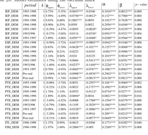
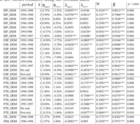
Table 2b. Model estimates using the German mark

period k φ_upper φ_lower λ_upper λ_lower α β ^p−value

IEP_DEM 1993-1998 1 4.75% -5.35% -0.0655*** -0.0346 0.1018*** 0.8012*** 0.000 IEP_DEM 1994-1998 1 5.99% -4.49% -0.0756*** -0.0612* 0.132*** 0.7986*** 0.004 IEP_DEM 1995-1998 1 9.03% 6.60% 0.1883*** 0.0059 0.1923*** 0.7628*** 0.000 IEP_DEM 1996-1998 4 8.90% 6.55% 0.0595 0.0052 0.2956*** 0.6569*** 1.000 IEP_DEM 1993-1995 1 -0.39% -4.47% -0.0055 -0.0828* 0.0545*** 0.9239*** 0.006 IEP_DEM 19931996 1 -0.37% -3.04% -0.0114 -0.0336* 0.0541*** 0.9321*** 0.004 IEP_DEM 1993-1997 1 3.89% -4.06% -0.059*** -0.0488* 0.0288*** 0.9566*** 0.006 ESP_DEM 1993-1998 1 -0.99% -3.72% -0.0473*** -0.0805*** 0.0942*** 0.9186*** 0.000 ESP_DEM 1994-1998 1 0.83% -5.70% -0.0628*** -0.102*** 0.1257*** 0.8968*** 0.004 ESP_DEM 1995-1998 1 1.04% 0.21% -0.0223 -0.0103 -0.0017*** 0.9986*** 0.038 ESP_DEM 1996-1998 1 1.16% 0.84% -0.024 -0.0125 0.1015*** 0.9016*** 0.000 ESP_DEM 1993-1995 1 -1.75% -7.99% -0.0664 -0.5411*** 0.1319*** 0.8391*** 0.010 ESP_DEM 19931996 1 -1.60% -6.44% -0.0237* -0.1449*** 0.2226*** 0.7174*** 0.018 ESP_DEM 1993-1997 1 0.70% -4.03% -0.0665*** -0.078*** 0.1081*** 0.8963*** 0.000 ESP_DEM Pre real 1 -4.04% -8.34% -0.0988*** -0.4876*** 0.2962*** 0.7747*** 0.004 ESP_DEM Post real 1 0.99% -1.74% -0.0461** -0.0815*** 0.0138*** 0.9813*** 0.000 PTE_DEM 1993-1998 1 -0.08% -3.74% -0.0031 -0.2597*** 0.104*** 0.9069*** 0.002 PTE_DEM 1994-1998 1 -0.32% -3.32% -0.0023 -0.1757*** 0.1092*** 0.9024*** 0.008 PTE_DEM 1995-1998 1 1.76% 1.14% -0.0553 -0.0112* 0.0734*** 0.927*** 0.018 PTE_DEM 1996-1998 1 1.89% -0.26% -0.0694* 0.0016 0.0821*** 0.9204*** 0.016 PTE_DEM 1993-1995 1 -3.69% -4.52% -0.0088 -0.7588*** 0.1594*** 0.8379*** 0.000 PTE_DEM 19931996 1 -0.79% -3.88% -0.1195 -0.3029*** 0.1065*** 0.8947*** 0.000 PTE_DEM 1993-1997 1 0.09% -3.88% -0.0328** -0.3086*** 0.1037*** 0.8937*** 0.000 PTE_DEM Pre real 1 -3.28% -4.62% -0.0145 -0.0916 0.209*** 0.8215*** 0.000 PTE_DEM Post real 1 -0.31% -1.86% -0.0019 -0.0977*** 0.0649*** 0.9354*** 0.010 ITL_DEM 1996-1998 1 1.37% 0.99% -0.0615 -0.0306 0.1771*** 0.8302*** 0.040 FIM_DEM 1996-1998 1 1.97% 1.60% -0.2884*** -0.005 0.2269*** 0.7971*** 0.008

Notes: as for Table 2a.

Table 3. Model estimates using the median currency, March 1, 1996 to February 28, 1998

k φ_upper φlower λupper λlower α β p−value

ATS_MED 2 -0.02% -0.28% -0.5608*** -0.0903 0.4342*** 0.701*** 0.002 BEF_MED 2 0.00% -0.29% -0.0712*** -1.2519*** 0.3596*** 0.4464*** 0.004 NLG_MED 2 0.39% 0.00% -0.0055 0.0005 0.4888*** 0.4986*** 0.004 DKK_MED 8 -0.29% -1.23% 0.0081 -0.2593 0.208*** 0.8211*** 0.000 DEM_MED 3 -0.04% -0.26% -0.7665*** -0.3688*** 1.0702*** 0.3854*** 0.000 FRF_MED 1 -0.74% -1.02% -0.0186** -0.0137 0.2769*** 0.769*** 0.002

ESP_MED 1 1.09% 0.59% -0.0424 -0.0195 -0.0043 1.0006*** 0.000

PTE_MED 1 1.73% 0.58% -0.0633 -0.0694*** 0.1447*** 0.8717*** 0.002 IEP_MED 1 9.18% 6.80% 0.2163*** 0.0001 0.197*** 0.7524*** 0.000 ITL_MED 1 0.94% 0.35% -0.1091 -0.0812 0.1682*** 0.8416*** 0.010 FIM_MED 1 1.28% 0.86% -0.0866*** -0.0659 0.2005*** 0.8262*** 0.004

Notes: as for Table 2a. The period begins on October 4, 1996 for Finland and on November 15, 1996 for Italy.

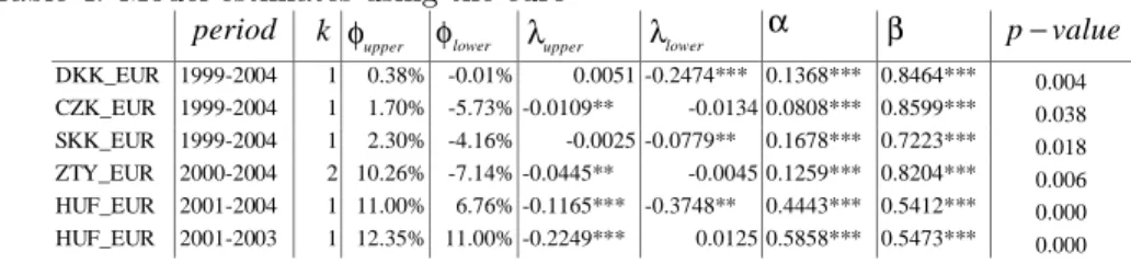
Finally, we now turn to the estimation results for the currencies expressed against the euro, for the period 1999 to 2004. During the period when the

Danish krone was in ERM-2, the estimated bandwidth decreases further from the 0.8% …gure, reported above, in the original ERM period to 0.4%. However, the mean reversion coe¢ cient bears the correct sign and is signi…cant only for the lower bound.

For the CEE countries against the euro we …nd the following. Hungary is an interesting case because on May 4, 2001, it widened the ‡uctuation bands around the central parity.³¹ From May 2001 to April 2004, the estimated up- per and lower thresholds were located, respectively, 11% and 6.76% away from the central parity (both on the stronger side of the o¢ cial ‡uctuation band of 15%). The mean reversion coe¢ cients have a negative sign and are signi…cant.

This would seem to give strong support for the fact that exchange rate policy targeted a narrow band, which it judged compatible with the in‡ation target.

However, this is only part of the story. On June 4, 2003, the central parity was devalued by some 2.26%, which triggered considerable depreciation of the currency inside the band. Looking at the period from May 4, 2001 to June 3, 2003 reveals that until the devaluation of the central parity, mean reversion was signi…cant only on the upper (stronger) threshold. So, mean reversion to the lower threshold detected for the whole period may refer to the post-devaluation period.

According to the statement of the Monetary Council of the National Bank of Hungary, dated August 18, 2003, “the Monetary Council puts the equilibrium exchange rate, which foster rapid economic growth without endangering price stability in the range of 250 to 260 forints per euro”. Relative to the then prevailing central parity of 282.36 forint per euro, this means a band of 7.92%

to 11.46% on the stronger side of the o¢ cial ‡uctuation margins. Thus, the estimated band for the whole period from 2001 to 2004 (upper bound=11%;

lower bound=6.76%) is broadly in line with the implicit target of the Hungarian monetary authorities.

As shown earlier, a special case of the Delgado-Dumas solution is tantamount to managed ‡oating without o¢ cially announced target zones, which could also induce some non-linear behaviour in the exchange rate. In particular, if the monetary authorities are targeting an implicit target zone, the SETAR model should be particularly useful to detect it because in such a case, interventions would be undertaken only if a depreciation or appreciation of the nominal ex- change rate exceeded a given pain threshold of the monetary authorities. This may be the case of the Czech Republic and Slovakia, which have de jure and de facto managed ‡oating. Notwithstanding the o¢ cial free ‡oating regime of the Polish zloty vis-à-vis the euro, we may still expect some mean reversion behaviour towards a band of inaction. Results reported in Table 4 con…rm our suspicion about the presence of non-linear behaviour. However, the mean re- version appears to be one-sided. There are signs of signi…cant mean reversion

3 1Note that the crawling peg system was abandoned only on October 1, 2001. However, at the time of the widening of the ‡uctuation band from 2.25% to 15%, the rate of crawl was already very low, 0.00654% a day, amounting to a total devaulation of the central paritiy of around 1.12% until October 1, 2001. Therefore, we believe that this did not have an impact on the behaviour of the exchange rate within the band.

only on the strong side for the Czech Republic and Poland, and only on the weak side for Slovakia. The mean reversion of the Czech koruna and the Polish zloty may actually re‡ect the recent switch from huge nominal appreciation to a large depreciation of the two currencies. The width of the estimated band is close to 7% for the Czech Republic and Slovakia, which is in sharp contrast with the detected wide band of more than 17% for Poland, lending more empirical support for more active exchange rate policies in the two former countries.

Likewise for the period preceding the introduction of the euro, there appears to be strong integrated GARCH e¤ects in the conditional variance for all cases.

Table 4. Model estimates using the euro

period k φ_upper φlower λ_upper λlower α β p−value

DKK_EUR 1999-2004 1 0.38% -0.01% 0.0051 -0.2474*** 0.1368*** 0.8464*** 0.004 CZK_EUR 1999-2004 1 1.70% -5.73% -0.0109** -0.0134 0.0808*** 0.8599*** 0.038 SKK_EUR 1999-2004 1 2.30% -4.16% -0.0025 -0.0779** 0.1678*** 0.7223*** 0.018 ZTY_EUR 2000-2004 2 10.26% -7.14% -0.0445** -0.0045 0.1259*** 0.8204*** 0.006 HUF_EUR 2001-2004 1 11.00% 6.76% -0.1165*** -0.3748** 0.4443*** 0.5412*** 0.000 HUF_EUR 2001-2003 1 12.35% 11.00% -0.2249*** 0.0125 0.5858*** 0.5473*** 0.000

Notes: as for Table 2.