This version is a draft. Please DO NOT QUOTE without the authors’ permission
How does knowledge spur economic growth?
The contribution of universities and the importance of geographical space
Tommaso Agasistia ,Cristian Barrab &Roberto Zottib
aDepartment of Management, Economics&Industrial Engineering, Politecnico di Milano, P.za Leonardo da Vinci, 32, 20133, Milano, MI, Italy
bDepartment of Economics and Statistics, University of Salerno, Via Giovanni Paolo II, 132, 84084, Fisciano, SA, Italy
Paper prepared for the 4th Workshop on Efficiency in Education Politecnico di Milano School of Management October 20th and 21st, 2016
ABSTRACT
In this paper, we test whether there is a link between the performance of universities and the economic growth where they operate. We specify a growth model where the ratio at which universities are able to convert inputs into outputs has been measured taking into account the traditional role of universities (i.e. teaching and research) as well as the knowledge transfer through which they interact with the communities. The model is estimated on panel data over the period 2006 to 2012. The evidence suggests that the presence of universities fosters local development, validating the use of university efficiency as an instrument able to capture the impact on the community of the ability of universities of making the most with the available resources; knowledge spillovers occur between areas through the geographical proximity to the efficient universities, suggesting that the geography of production is affected, mainly when all the three mission of universities are taken into account.
Keywords: Higher education; Knowledge spillovers; Local economic development; Parametric technique.
JEL-Codes: I21; C14; C67
1. INTRODUCTION, MOTIVATION AND RESEARCH QUESTION
The assumption that universities could and should contribute to the social, economic and cultural development of the territories in which they operate is widely accepted nowadays. Several theoretical paradigms have been inspired by the positive role that Higher Education Institutions (HEIs) can play in the interaction with key stakeholders, with the final aim of transferring knowledge, disseminating culture and foster economic competitiveness.
Among the first attempts of defining the “external” role of HEIs, the famous Clarke’s triangle (Clarke, 1986) stands as a model for interpreting the performances of HE systems. In the author’s view, the activities and results of universities are not only the fruit of the academic quality and willing, but are instead also influenced by the interplay with the “State” (i.e. the government that regulates the system) and the “market”, intended in its inclusion of various actors, from students/families to public and private entities of the territory. At the same time, the outcome of the universities’ operations is not confined to the boundaries of academia, but exerts a positive/negative influence (depending on its quality) on wider society and economy. Later in the literature, a clear indication emerges: that it is possible to theoretically define a specific “external”
impact of teaching and research on the community – and, such impact can actually be measured empirically. Bornmann (2013), for example, reviews two decades of studies that attempt at estimating the “societal impact” of research, defining the concept as the ability of transforming knowledge into economically relevant products, services and processes. Even more compelling becomes the notion that universities can contribute to the improvement of human capital, which in turns can stimulate and foster economic growth – see, for example, Benhabib & Spiegel (1994) and Barro (2001). The most recent development in the field is the formalization of the specific role of universities in sustaining local development into a stand- alone new “mission” that must be added to the traditional two (teaching and research). Researchers often use the terms
“third mission” (Laredo, 2007) or “knowledge transfer” (Bekkers & Freitas, 2008) to identify the new set of activities which, all together, constitute the various channels through which HEIs interact with the communities where they are immersed, and contribute to their economic and social development. In the remainder of the paper, we adopt the expression of “third mission” (or TM) as the preferred one, for guaranteeing homogeneity and univocal naming in the discussion of results.
Quality of operations matter, however. While early indicators of “third mission” tried to capture the amount of teaching and research conducted in a given territory, and to correlate it with indicators of economic growth, the approach is substantially different now. The availability of new reliable and more complete datasets, coupled with advancements in theoretical frames, allows the analysts to describe much more precisely the channels through which HE influences the territorial social and economic development. First, measures of human capital development and research can be collected at the level of single institutions, and not only at a more aggregated level as district, province, region, country. Second, several databases also include indicators about the kind of actions that universities conduct with respect to third mission, thus enabling the inclusion of this area of activities into the wider picture of HEIs’ performance. Third, the studies about HE operations highlighted how HEIs tend to operate inefficiently in many cases, in other words using more resources than needed to obtain the observed levels of output – if the resources themselves would be used in their most productive way (a discussion is in Johnes, 2006). In this perspective, more precise information about the role of universities in developing human capital should consider not only their performance levels, but also the level of efficiency at which they operates, in other words the ratio at which they are able to convert inputs (human and financial resources) into outputs (as for instance graduation rates, publications, technology transfer initiatives). There are few examples of studies that take into consideration these potential
This version is a draft. Please DO NOT QUOTE without the authors’ permission
advantages for empirical analyses. For instance, Branwell & Wolfe (2008) conduct a case study to show how a specific university acts in fostering economic growth in the Region where is located. On a related ground, Etzkowitz (2003) formulates a theory about how specifically the third mission of universities can contribute to the economic development (‘entrepreneurial university’), and many subsequent works demonstrate the empirical validity of the intuition. Barra & Zotti (2016) use the number of Italian graduates and universities’ efficiency scores as (institution-level) indicators of human capital, and demonstrate their positive effect on the areas where HEIs operate. This paper constitutes a natural key reference, as our study moves from it to extend and improve the preliminary analyses presented there.
In this paper, we contribute to the advancement of the literature by proposing an empirical analysis about the impact of Italian universities’ performance on local GDP growth. Specifically, we address the following research question: is there a statistical link between the performance of universities and the economic growth of the geographical area where they operate? We provide an answer to the research question by employing an econometric analysis, which uses a dynamic panel model for the period 2006-2012. Data refer to 53 public universities, and to 46 Italian Provinces. The efficiency of universities is estimated by means of an innovative and robust Stochastic Frontier Analysis, and takes into account indicators of all the three missions – teaching, research and TM. Such a measurement of efficiency makes it more complete than the one proposed by Barra & Zotti (2016), in which the dimension of third mission is completely missing.
The topic addressed in this paper is of particular, timely interest in the current situation of Italian economy. On one side, Italian governments struggled for decades in searching for policy interventions to launch the competitiveness of the country.
Our findings point at the use of the educational instrument for fostering economic development, by reinforcing the nexus between human capital – favoured by universities’ performances – and economic growth. On the other side, the recent public debate has been centred on raising the efficiency of public spending (Arena & Arnaboldi, 2013), and HE sector was also included in this wider effort – indeed, public expenditure in the sector amounts almost 1% of GDP (OECD, 2016). The results of our empirical analysis demonstrates that it is not only universities’ performance that matters, but especially their efficiency, i.e. their ability of making the most with the available resources.
2. UNIVERSITIES AND ECONOMIC GROWTH
The impact of universities on regional development has been the object of intense debate in the last years in order to underline whether the economic growth and prosperity of regions could be attributable to the presence of a university.
Several are the contributions that universities can make in order to increase local economic development such as the knowledge transfer through education and human resources development (i.e. human capital of students and graduates), knowledge creation and regional innovation through research (i.e. publications) and technology transfer (i.e. third mission) activities, all leading to spillover effects and regional competitiveness (see Drucker and Goldstein, 2007, for a review of the current approaches to assess the impact of universities on regional economic development).
A key contribution of the universities to local development is related to the teaching mission of the universities which may lead to important and strong territorial effects on the extent that higher education institutions play an important role in providing knowledge spillovers through human capital embodied in graduating students as the move from universities to firms. Indeed, highly skilled and well-educated individuals are one of the main outputs of universities and are considered as an important drive of economic development (Florida et al. 2008) as well as one of the most relevant channels for propagating and commercializing knowledge from the academia environment to local high technology industry (Varga,
2000; Robert and Eesley, 2009; Stephan, 2009). Bauer, Schweitzer, and Shane (2012) demonstrate that concentrations of college graduates in some American states increased their per capita incomes and slowed down income convergence across states. Riddel and Schwer (2003) find that the most significant positive contribution made by the universities to innovation, and to generating and transmitting knowledge, are attributable to university graduates. Graduates may decide to start up new firms that boost the dynamics of the local economic environment (Florax 1992; Goldstein et al. 1995) as well as increase the innovativeness, creativity and productivity of local firms (Rothaermal and Ku, 2008) and full-time highly-skilled employees are key factors for increasing the number of spin-offs (Algieri et al. 2013). As a consequence, regions that increase the average level of education of their employees tend to introduce novelties in their existing industrial texture and become more innovative (Chi and Qian, 2010; Gumbau-Albert and Maudos, 2009). According to Haapanen and Tervo (2012) “the most competitive regions are typically those with high levels of human capital” and “universities play a key role in bringing the human capital into regions”. Importantly, such supply skilled labour benefit is, to a certain degree, localised as the mobility of graduates is limited and knowledge spillovers are shaped by geographic proximity (Boschma, 2005; Salter and Martin, 2001); indeed, as a high proportion of graduates look for a job in the region where they receive education (Felsenstein, 1995; Glasson, 2003; Breschi and Lissoni, 2008) or at least they do not move from the region of studies within ten years from after graduation, firms situated close to universities may have easy access and take advantage of the knowledge generated.
Knowledge spillovers from universities to firms involve also research published in scholarly journals (i.e. codified knowledge). Although this kind of knowledge can be easily transferred at low cost (i.e. download from internet) and therefore orthogonal to firm location, research in social sciences is less codified and attract innovative startup (Calcagnini et al. 2016) and the proximity to high output universities may important for accessing social science research (Audretsch et al.
2005). The higher is the quality of academic research, the larger is the contribution to industrial innovations (Mansfield, 1995) and to firms’ technological performance, even though considerable industry differences are measured (Leten et al.
2014). Scientific research results in knowledge that could lead to firms’ innovation activities (Bercovitz and Feld, 2007;
Autant-Bernard, 2001) or create and extend economic activities (Cohen et al. 2000). According to Goldstein and Renault (2004), universities’ research activities contribute to the creation of knowledge spillovers within the regional environment leading to an improvement of local economies; Chatterton and Goddard (2000), underline that HEIs should focus more on research activities and funding in order to respond to regional needs; Walshok (1997) focuses on the contribution that HEIs research activities could make in order to contribute to the local economic development such as, among others, new product development, industry formation, job creation and access to advanced professional and management services. Del Barrio- Castro and García-Quevedo (2005) find that university research has a positive impact on the regional distribution of innovation. Empirical evidence from firm surveys (Mansfield, 1995, 1997; Cohen et al. 2002; Veugelers and Cassiman, 2005) confirms the importance of university research for corporate innovation performance.
Universities, in addition to the traditional teaching and research activities, try to attain a high interaction with the society by building a link between research and business through patents, business incubators, collaboration agreements and spin-offs.
The contribution of universities to local development is always more frequently focused on the technology transfer channel, highlighting the importance of HEIs services for the industry sector and specifically for boosting the innovation activities of the firms. Indeed, universities are investing specific resources to these activities in order to promote knowledge transfer and as, a consequence, the university-industry relationship has become more important due to the role played by technological progress in the development of an area (Algieri et al. 2013; Muscio, 2010; Guldbrandsen and Smeby, 2005). The establishment of new companies based on technologies derived from university research is a well-recognized driver of
This version is a draft. Please DO NOT QUOTE without the authors’ permission
regional economic development (Hayter et al. 2016). Knowledge transfers from academia has been investigated through licensing (Shane, 2002), academic spin-off activities (Shane, 2002) and citation to academic patents (Henderson et al. 1998). Incubators are effective in supporting new entrepreneurial initiative (Auricchio et a. 2014) and innovative start- ups are also an effective way to facilitate technology transfer from the university to the economy (Boh et al. 2015).See Maietta (2015), on the channels through which university–firm R&D collaboration impacts upon firm product and process innovations, and Caniëls and van den Bosch (2010), on the role of higher education institutions (HEIs) in building regional innovation systems. The spatial pattern of knowledge (i.e. the importance of geographic location) plays an important role; indeed the knowledge flows tend to be restricted to the area where the university is located and firms likelihood of innovating is positively affected by their proximity to a university (Piergiovanni and Santarelli, 2001). This pattern is confirmed by empirical evidence that shows how firms tend to locate their production in proximity of universities as they as easier access to the knowledge generated by tertiary education. In other words, geographical proximity is a channel through which knowledge and technology could be transferred from the universities to the industry sector, representing an important contribution to regional economic development. On the presence of localized knowledge spillovers from university research and on the role of geographic proximity in firm-university innovation linkages see also D’ Este et al. (2012) and Abramovsky and Simpson (2011).
3. EMPIRICAL STRATEGY
3.1. LOCAL ECONOMIC DEVELOPMENT
In order to analyse the relationship between the efficiency of universities and local economic growth, we specify the following dynamic panel model (for a similar approach but in a different environment see Hasan et al. 2009, and Destefanis et al. 2014; Barra and Zotti, 2016):
𝑙𝑛 𝐺𝐷𝑃𝐶',),*= 𝛼𝑙𝑛𝐺𝐷𝑃𝐶',),*./+ 𝛽/𝑙𝑛𝐸𝐹𝐹',),*+ 𝛽4𝑙𝑛 𝐸𝐹𝐹',),*∗ 𝑊 + 𝛽7𝑙𝑛𝐿𝐹',),*+ 𝛽9𝑙𝑛𝑀𝐾',),*+ 𝛽<𝐿𝐺 + 𝜇',)+ 𝜏*+ 𝜀',),* (1)
where 𝑙𝑛 is the natural logarithm, 𝐺𝐷𝑃𝐶 is gross domestic product per capita (measured as the sum of the gross values added of all units divided by population in each area where the university is located1) explained by 𝐺𝐷𝑃𝐶*./ (its lagged value), by 𝐸𝐹𝐹 (efficiency of universities), by 𝐸𝐹𝐹 ∗ 𝑊 (spatial lagged value of the HEIs efficiency estimates), by 𝐿𝐹 (share of the labour force with a university degree as proxy of the quality of the labour market), by 𝑀𝐾 (market share measured as the ratio between the number of enrolments at university 𝑖 and the total number of enrolments in the universities located in the same province, included for capturing the potential effects due to the presence of more concentration or competition between universities) and by LG (number of employed individual at time 𝑡 minus the number of employed individual at time 𝑡 − 1); 𝜇 is the unobserved area-specific effect, 𝜏 are year dummies controlling for time- specific effect, and finally 𝜀 are the disturbance erros. Subscripts 𝑖, 𝑗 and 𝑡 refer to the unit of analysis (universities), area where the university is located and time periods (years), respectively. We have a highly detailed spatial stratification than enables us to capture the differences between geographical areas and to obtain more accurate estimates. Specifically, our analysis is fully conducted on a local basis to accurately capture the contribution of HEIs. More specifically, GDPC and LG are not measured at the national level as in previous studies, but at the local level such as at SLL level (SLL stands for a
1GDP per worker is constructed by updating the SLL value-added data from ISTAT through the period of 2006 to 2012 with data from the Bureau van Dijk AIDA data set (similar to Destefanis et al 2014, Barra and Zotti, 2016) (AIDA is a database providing balance sheets and other information about Italian firms with a turnover of at least one million euro. See for further information: http://aida.bvdep.com/).
group of municipalities - akin to the UK’s Travel-to-Work-Areas - adjacent to each other, geographically and statistically comparable, characterized by common commuting flows of the working population). In our opinion, two are the main advantages of using some data at such disaggregated level; first of all, we are able to better underline the economic performances across the Italian territory; indeed, according to the Italian Statistical Office (ISTAT) , the SLL represents the place where the individuals live and work and, above all, where take place their economic and social relationships. SLLs have been constructed considering daily commuting flows for working reasons; in other words they have been build taking into account the number of employees who daily reach the working place and then go back home2. Secondly, the other advantage of having information of the above described variables at SLL level is that we assign almost to each university a unique value of the environmental variables; the only exception consists in those areas like Rome, Naples or Milan where more than one university is located (for instance the same value of GDPC or LG is assigned to each university in Rome).
This allows us to better capture the differences across geographical areas and to consider in some detail how the performances of HEIs influence local growth3. Moreover, the idea of such disaggregated territorial level is not completely new in the literature. McHenry (2014), with the aim of investigating the geographic distribution of human capital in US, use the commuting zone described as a collection of counties making up a coherent local economy—as the location measure.
He stated that, although states tend to be larger and thus offer more data for measurement, they are poor proxies for local labor markets. Therefore, he consider the smallest geographic space where most residents work and most workers reside such as the commuting zone being a collection of counties (or single county) that share particularly strong commuting links4. This means that, for each university in the sample, we are able to match a value of GDPC and LG corresponding to the municipality where the university is located. MK is also measured at university level. LF is measured, instead, at regional level (because not available at a more disaggregated level).
To eliminate 𝜇', the unobserved area-specific effect, and given the dynamic panel specification of the model, we use the two-step system GMM estimator with Windmeijer (2005) corrected standard error in dynamic panel specification developed by Arellano and Bond (1991), Arellano and Bover (1995) and Blundell and Bond (1998). Moreover, in order to deal with suspected endogeneity problem between the efficiency of the universities and economic growth (i.e. for instance changes in the economic conditions could lead to an increase in the demand or supply of graduates) we include lagged levels and differences as instruments of 𝐸𝐹𝐹.
Specifically, in order to examine whether geographical space has an impact on the relationship between the efficiency of the universities and local economic growth, we specify a spatial-lag model such that the efficiency levels of the HEIs can spill over to the area 𝑗; in other words, we take into account that growth in area 𝑗 depends systematically on the human capital
2In the census of the population made by ISTAT, among the SLLs located, in more that 330 of them (thus more than 70% of the population), more the three quarter of the individual employed live and work in the same SLL.
3 In order to underline why we think the last point is very important in our empirical framework, take for instance one of the representative regions in the North-Central part of Italy such as Emilia Romagna. In Emilia Romagna, the main universities are the University of Bologna (located in the city of Bologna), the University of Ferrara (located in the city of Ferrara), the University of Modena (located in the area of Modena) and the University of Parma (located in the city of Parma). When constructing the dataset, we assigned a value of GDP to each university according to the location where the university is placed. If we had considered values of GDP at regional level, we would have assigned the same value to all the universities located in the region of Emilia Romagna; instead, by proceeding using SLL, the University of Bologna gets the value of GDP corresponding to the municipality where Bologna is located, the University of Ferrara gets the value of GDP where the city of Ferrara is located, the University of Modena gets the GDP value when the city of Modena is located and finally the University of Parma gets the GDP value of the municipality where the city of Parma is located.
4 Considering a different scenario, such as the financial system, the SLL geographical measure data had already been used in the literature; indeed, Destefanis et al. (2014), with the aim of explaining the nexus between local financial development and economic growth, rely upon Italian data highly disaggregated at the territorial level such as SLL. According to them, this high level of disaggregation allows to decisively reduce the potential role of omitted time invariant factors.
This version is a draft. Please DO NOT QUOTE without the authors’ permission
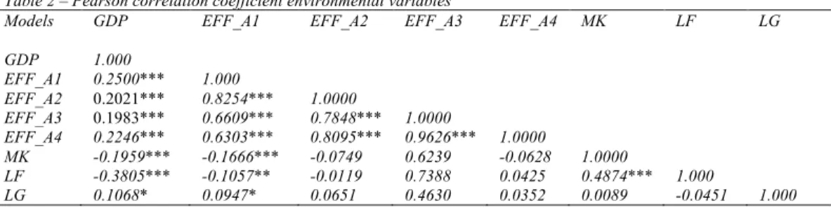
development in neighbouring areas 𝑗 ∈ 𝐽, where 𝐽 is the set of all areas (Anselin, 1988). We use an inverse distance weighed matrix to weight 𝐸𝐹𝐹 of all neighboring areas. In matrix notation, 𝐸𝐹𝐹 ∗ 𝑊 is the weighted average of university efficiency proxies across 𝐽) areas neighboring area 𝑗. In other words, the spatial weight matrix is assumed to reflect the geographical structure of the knowledge spillover mechanisms operating at local level. The parameter we are most interested in is 𝛽4 which measures whether economic growth at community level benefits (𝛽4> 0), suffers (𝛽4< 0) or is independent (𝛽4= 0) from the university efficiency (due to the presence of the universities with a high level of efficiency) of neighbours. As usual, we check the correctness of the model through the Sargan test of over-identifying restrictions for validity of the instruments, while the Arellano-Bond test is, instead, used for testing the autocorrelation between the errors terms over- time. See Tables 1 and 2 below for a description of the variables used as controls and for hteir correlation coefficiencts. In estimating the GMM model we rely on STATA 125.
[Tables 1 and 2 around here]
3.2. UNIVERSITY EFFICIENCY
We calculate a university’s relative efficiency in converting inputs into a production set while maximizing outputs. The idea is that an area in which universities comply with their functions (i.e. producing highly skilled and well-educated individuals, highly rated research and knowledge transfer) with the utilization and the combination of different resources is on average more efficient than other areas and should benefit in terms of growth because they contribute to increasing local human capital.
In literature, two main methods have been extensively applied for measuring efficiency: non-parametric6 and parametric7. There is no general consensus about which method is to be adopted to measure higher education institutions efficiency.
These two main approaches have not only different features, but also advantages and disadvantages (Lewin and Lovell 1990). On one hand, the non-parametric method does not require the building of a theoretical production frontier, but the imposition of certain, a priori, hypotheses about the technology (free-disposability, convexity, constant or variable returns to scale). However, if these assumptions are too weak, the level of inefficiency could be systematically under-estimated in small samples, generating inconsistent estimates. Furthermore, this method is very sensitive to the presence of outliers. On the other hand, the parametric method uses a theoretical analysis to construct the efficient frontier, it’s not sensitive to extreme values because imposes some assumptions on the error distribution, but must deal with the problem of decomposing the error term. In particular, SFA, proposed by Aigner et al. (1977), Meeusen and Van den Broeck (1977) and Battese and Corra (1977), assumes that the error term is composed by two components with different distributions (see Kumbhakar and Lovell (2000) for analytical details on stochastic frontier analysis). The first component, regarding the
“inefficiency”, is asymmetrically distributed (typically as a semi-normal), while the second component, concerning the
5 Coordinates of the areas where universities are located have been extracted from the mapping ISTAT website (http://www.istat.it/it/strumenti/cartografia). The spatial weights matrix has been constructed using the module so called "spwmatrix" by Jeanty (2010a). The spatial weights matrix is row-standardized, i.e. the elements of each row sum up to one. Instead, the spatial lagged variables involved in the analysis, i.e. HCQ and GDPC, was built using the module so called "splagvar" by Jeanty (2010b).
6Such as the DEA (Data Envelopment Analysis) and FDH (Free Disposable Hull), proposed by Charnes et al. (1978) and due to the original contribution of Farrell (1957), based on deterministic frontier models (see also Cazals et al. 2002).
7 Such as Stochastic Frontier Approach (SFA), Distribution-Free Approach (DFA) and Thick Frontier Approach (TFA), based on stochastic frontier models (see Aigner et al. 1977).
“error”, is distributed as a white noise. In this way, it is necessary to assume that both components are uncorrelated (independent) to avoid distortions in the estimates8.
In this paper, we prefer to employ a Stochastic Frontier Analysis because it offers useful information on the underlying education production process, as well as information on the extent of inefficiency9. Nowadays, the most widely applied SFA technique is the model proposed by Battese and Coelli (1995) to measure technical efficiency across production units.
Intuitively, technical efficiency is a measure of the extent to which an institution efficiently allocates the physical inputs at its disposal for a given level of output. On a methodological ground, the most recent literature, which deals with panel data, emphasized the importance of separating inefficiency and fixed individual effects. Indeed, the efficiency scores may suffer from the presence of incidental parameters (number of fixed-effect parameters) or time-invariant effects, often unobservable, that may distort the estimates (Greene, 2005; Wang and Ho, 2010). For instance, students’ or researchers (average) innate ability may be an important determinant of their individual academic achievement and thus account for an important share of the heterogeneity in data when evaluating the efficiency of the institution in which they are studying or working. As Wang and Ho (2010) have underlined: “(…) stochastic frontier models do not distinguish between unobserved individual heterogeneity and inefficiency”, forcing “all time-invariant individual heterogeneity into the estimated inefficiency”. In order to deal with this problem and to estimate the technical efficiency, we apply a procedure developed by Wang and Ho (2010), according to whom after transforming the model by either first-difference or within-transformation, the fixed effects are removed before estimation. More specifically, we impose to data a within transformation. As Wang and Ho (2010) specified, “by within-transformation, the sample mean of each panel is subtracted from every observation in the panel. The transformation thus removes the time-invariant individual effect from the model”. Following the notation in Wang and Ho (2010), the transformation employed in our model is (being 𝑤, for instance, any input or output to be transformed):
𝑤'.= 1/𝑇 𝑤'*, 𝑤'*.= 𝑤'*− 𝑤'.
R
*S/
(2)
The stacked vector of 𝑤'*. for a given i is:
𝑤'.= (𝑤'/., 𝑤'4., … , 𝑤'R.)U (3)
For simplicity, hereafter in our formulation does not include a subscript t10. The baseline model associated to distance function after the transformation can be written as:
8Instead, DEA, unlike SFA, assumes that the “error” is fixed over time, while the “inefficiency” component is normally distributed.
Finally, TFA assumes that the radial distance between the efficient frontier and the lowest and highest quartile is the white noise, while the deviation between the two quartiles indicates inefficiency.
9Apart from the strict statistical distinctions between the two type of approaches, an important reason according to which a Stochastic Frontier Analysis (SFA) has been applied, instead of a Data Envelopment Analysis (DEA), is the need of keeping the empirical analysis as a parametric estimation. Indeed, as specified in the paper, the analysis is performed in two stages: firstly, we use a Stochastic Frontier Analysis (SFA) to calculate an index of efficiency for each university and secondly, a growth model is tested, through a system generalized method moment (sys-GMM) estimator, to measure the effects of the human capital development on local growth. As the GMM is a parametric method, we decide to keep parametric also the measure of the higher education institutions and therefore to apply a Stochastic Frontier Analysis.
10Even though the formulation does not include a subscript 𝑡, the inefficiency component is time varying in order to examine how the (in)efficiency changes over time.
This version is a draft. Please DO NOT QUOTE without the authors’ permission
𝑓 𝑦'. = 𝑓 𝑥/., … 𝑥Y. + 𝜀'. (4)
where 𝑦 represents the conventional outputs, 𝑥 denotes the conventional inputs and 𝜀 denotes the disturbance term.
With stochastic frontier analysis, a frontier is estimated on the relation between inputs and outputs. This can be, for example, a linear function, a quadratic function or a translog function. This paper uses a translog function even though there is no general consensus about which one has to be adopted in the higher education environment (for a discussion on the different function forms, see Cohn and Cooper, 2004 and Agasisti and Johnes, 2009). However, concerning the structure of production possibilities, a more general functional form, that is, the transcendental logarithmic, or “translog”, could be considered for the frontier production function. The translog functional form may be preferred to the Cobb–Douglas form because of the latter restrictive elasticity of substitution and scale properties, and it allows for non-linear causalities, compared with the more simple Cobb-Douglas function (see Agasisti and Haelermans, 2015, who use a translog function in order to compare the efficiency of public universities among European countries)11.
Following common practice, we now assume a translog functional form for the output distance function:
𝑙𝑛𝐷'.Z = 𝛼[
\
[S/
𝑙𝑛𝑦['.+ 𝛽]
^
]S/
𝑙𝑛𝑥]'.+1
2[ 𝛼[Y𝑙𝑛𝑦['.𝑙𝑛𝑦Y'.+ 𝛽]a𝑙𝑛𝑥]'.𝑙𝑛𝑥a'.
b
)S/
^
]S/
c
YS/
\
[S/
]
+ 𝛿][𝑙𝑛𝑥]'.𝑙𝑛𝑦['.
\
[S/
^
]S/
(5)
By within transformation, 𝛼' (intercept that changes over time according to a linear trend with unit-specific time-variation coefficients and that represents time-invariant effects) disappears from our specification. In addition, time dummies are also included in the model in order to capture exogenous factors that might affect the production set. Normalizing by 𝑦', that guarantees the linear homogeneity of degree 1 in outputs12 ( \[S/𝛼[= 1) as suggested by Lovell et al. (1994), and imposing the linear ( \[S/𝛼[Y = 0 and \[S/𝛿][ = 0) and suitable symmetry restrictions (𝛼[Y= 𝛼Y[ and 𝛽]a = 𝛽a]), the output oriented distance function becomes:
𝑙𝑛 𝐷'.Z
𝑦'. = 𝛼[𝑙𝑛𝑦['.∗
\
[S/
+ 𝛽]
^
]S/
𝑙𝑛𝑥]'.+ 1/2[ 𝛼[Y𝑙𝑛𝑦['.∗ 𝑙𝑛𝑦Y'.∗ + 𝛽]a𝑙𝑛𝑥]'.𝑙𝑛𝑥a'.
b
)S/
^
]S/
c
YS/
\
[S/
]
+ 𝛿][𝑙𝑛𝑥]'.𝑙𝑛𝑦['.∗
\
[S/
^
]S/
(6)
where 𝑦['.∗ = 𝑦['./𝑦'., 𝑦Y'.∗ = 𝑦Y'./𝑦'. and thus 𝑦f.= 1. In addition, the time dummies are also taken into account in order to capture the technology change that can influence the production process of the decision-making units (i.e. universities). It’s obvious that 𝑙𝑛 𝐷'.Z is not observable. Then, in order to solve this problem, we can re-write 𝑙𝑛 𝐷'.Z/𝑦'. = 𝑙𝑛 𝐷'.Z - 𝑙𝑛 𝑦'. .
11On the other hand, see Laureti, 2008, who uses a Cobb-Douglas function in order to model exogenous variables in human capital formation.
12Generally,linear homogeneity of degree 1 in outputs also implies that the sum of alphas is equal to zero and the sum of deltas is null.
Thus, we transfer 𝑙𝑛 𝐷'.Z to the residuals, i.e. on the right and side of the equation (5), and −𝑙𝑛 𝑦'. as dependent variable (Coelli and Perelman, 2000). In our case, we follow Paul et al. (2000), i.e. imposing 𝑙𝑛 𝑦' . The equation (5) thus becomes:
𝑙𝑛 𝑦'. = 𝛼[
\
[S/
𝑙𝑛 𝑦['.∗ + 𝛽]
^
]S/
𝑙𝑛𝑥]'.+ 1/2[ 𝛼[Y𝑙𝑛 𝑦['.∗ 𝑙𝑛 𝑦Y'.∗ + 𝛽]a𝑙𝑛𝑥]'.𝑙𝑛𝑥a'.
b
)S/
^
]S/
c
YS/
\
[S/
]
+ 𝛿][𝑙𝑛𝑥]'.𝑙𝑛 𝑦['.∗ + 𝑣'− 𝑢'
\
[S/
^
]S/
(7)
where 𝑣 is the vector of random variables assumed to be i.i.d. 𝑁(0, 𝜎k4) and independent of the 𝑢 term which stands for inefficiency component. In particular, 𝑢 is assumed to be heteroscedastic and, in particular, distributed as 𝜎l4= exp 𝑧'; 𝜆 following a half-normal distribution, i.e. 𝑁s(0,1), where 𝑧' is a vector of exogenous variables employed to explain determinants of inefficiency, and 𝜆 denotes a vector of unknown coefficients. In this analysis, we do not impose the “scaling property” (for more details see Wang and Schmidt (2002), in the context of cross-sectional data, and Alvarez et al. (2006), in the panel data context); indeed, as underlined by Wang and Ho (2010), “whether the scaling property holds in the data is ultimately an empirical question”. In other words, we assume changes not only in scale but also in the shape of the inefficiency distribution. The validity of the heteroscedastic assumption is tested using a LR test which allows us to identify the fit of the model and to confirm the imposition of some explanatory factors in the variance of the inefficiency term. As already said, we estimate the function above described in a panel context, employing within transformation as recently suggested by Wang and Ho (2010) in order to eliminate the incidental parameters from our estimation, under the hypothesis of efficiency variability over time. Once singled out the best practice frontier from translog output distance function model, we compute the efficiency scores as deviations from this frontier.
The coefficients 𝛼, 𝛽, 𝛿, 𝜆 and technical efficiency are estimated through a maximum likelihood estimator (MLE) using the STATA 12 software13.
3.2.1. PRODUCTION SET AND SPECIFICATION OF THE MODELS
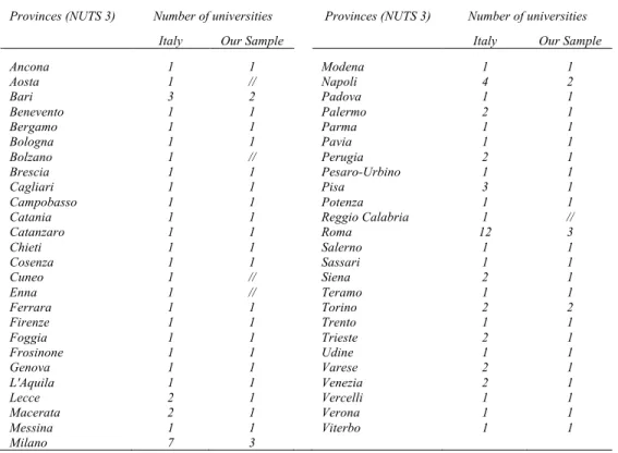
The dataset refers to 53 Italian public universities from years 2006 to 2012 (see Figure 1 for a map of Italy with the localization of universities included in the dataset) and it has been constructed using data which are publicly available on the National Committee for the Evaluation of the University System (CNVSU) website14. We exclude all private sector universities, owing to the absence of comparable data on academic research variables; this leaves us with a sample of 53 universities15, each of which yields data over the four year period, so we have a total of 212 observations (see Table 3 for the correspondence of universities and provinces in Italy and in our sample).
13The within transformation to data is employed using the “sf_fixeff” command as proposed by Wang and Ho (2010).
14 Data were obtained, not without some difficulties in the collection derived from the absence of a single database and the non- comparability of certain data. Unfortunately a longer period of data was not available to us. A drawback is represented by the fact that the years included in the analysis are recession years, whose consequence could affect university output in terms of, for example, research grants funded by private firms in the South of Italy.
15 Which is very representative of the higher education system in Italy, corresponding to almost 90% of the total number of public universities in the country. Confirming the representativeness of the sample used, in the 53 universities included in the empirical analysis are enrolled 88% of the students enrolled in the entire higher public education system in Italy.
This version is a draft. Please DO NOT QUOTE without the authors’ permission
[Figure 1 around here]
[Table 3 around here]
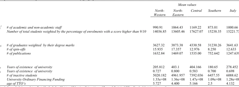
Referring to the literature on this subject, the production technology is specified, with two inputs: 1 – number of academic and non-academic staff; 2 - total number of students weighted by the quality of freshmen. More specifically, the first input is what we call the equivalent personnel (EQUIVPERS), namely the total number of academic staff and non-academic staff16; it is a measure of a human capital input and it aims to capture the human resources used by the universities for teaching activities17 (see Johnes, 2014; Agasisti and Dal Bianco, 2009). The second input is the total number of students weighted by the percentage of enrolments with a score higher than 9/10 in secondary school (STU_WEIGH)18. The total number of students measures the quantity of undergraduates in each university. Moreover, among the inputs that are commonly known to have effects on students’ performances there is the quality of the students on arrival at university; indeed, there is strong evidence that pre-university academic achievement is an important determinant of the students’ performances (Boero et al., 2001;
Smith and Naylor 2001; Arulampalam et al., 2004; Lassibille 2011). The underlying theory is that ability of students lowers their educational costs and increases their motivation (DesJardins et al., 2002). To take this into account, we weight the number of students by a proxy of the knowledge and skills of students when entering tertiary education. Thus, this input aims to capture both the quantity and the quality of students19.
Three measures of outputs are included in the model reflecting the teaching and research functions of HEIs20: 1 – number of graduates; 2 – number of publications; 3 – spin-offs. The first output is the number of graduates weighted by their degree classification (GRADMARKS), in order to capture the quantity and the quality of teaching and to treat in the same way quantity and quality in both the student input and output21 (see Kuah and Wong, 2011; Agasisti and Perez-Esparrells, 2010;
16We also consider non-academic staff in order to take into account the administrative staff who support the academic staff and the students.
17 The academic staff has been decomposed into three categories, namely professors, associate professors and researchers. In order to take into account this categorization, we assign weights to each category according to their salary and to the amount of institutional, educational and research duties the academic staff has to deal with (Madden et al. 1997) and assuming that a professor is expected to produce more teaching work than an associate professors and so on (Carrington et al. 2005). To the non-academic staff has been assigned the lower weight. Similarly to Halkos et al. (2012) we use the following aggregate measure of human capital input: Equivalent personnel (EQUIV_PERS)=1*professors+0.75*associate professors+0.50* researchers +0.25* non-academic staff. The weights have been chosen so that the distance between two ranks is 1/4=0.25. A potential limitation of this choice is represented by the decision to assign different weights. Therefore, for robustness, we also further test how alternative weights given to this variable would change the results, to avoid a sever discounting of researchers and non-academic staff. We firstly give the same weigh to each category. In other words, we assume that the categories of academic staff contribute in the same way as well as the non-academic staff: Equivalent personnel (EQUIV_PERS _2)=0.25*professors+0.25*associate professors+0.25* researchers +0.25* non-academic staff. Secondly, we suppose that both professors and associate professors contribute in the same way. Followed by researchers, and then by non-academic staff. Equivalent personnel (EQUIV_PERS _3)=1*professors+1*associate professors+0.75* researchers +0.50* non-academic staff. In all cases results (available on request) are similar.
18A similar measure is also used in Agasisti and Dal Bianco (2009). For robustness, we also weight total number of students by the percentage of enrolments from a Lyceum (i.e.non-vocational secondary school which are more academic oriented and specialized in providing students the skills needed in order to enroll in the university). Results, available on request, are similar.
19There are no measures of capital inputs (such as library, computing, buildings) which might have a role in determining university outputs; unfortunately such data are very difficult to obtain for Italy. This is confirmed by a recently published paper by De Witte and López-Torres (2015) in which they reviewed the literature regarding the efficiency in education. In describing the inputs in the education production function, only a very small amount of paper included those inputs in the analysis in higher education.
20 Unfortunately, due to the unavailability of data, we are not able to consider what is known to be the third function of the universities such as knowledge transfer to industry and links of HEIs with industrial and business surroundings.
21 For the readers who are not familiar with the characteristics of the Italian higher education system, in Italy students can graduate obtaining marks from 66 to 110 with distinction. This grade is calculated mainly according to the average grades students have obtained in the exams; then a certain number of points is added after the final dissertation has been graded. In order to weight the graduates according to their degree marks, we apply the following procedure: GRADMARKS =1* graduates with marks between 106 and 110 with
Thanassoulis et al. 2011; Duh et al. 2014). According to Catalano et al. (1993), “the task assigned to university is to produce graduates with the utilization and the combination of different resources” and Madden et al. (1997) used the number of graudates under the hypothesis that the higher is the number of graduates, the higher is the quality of teaching. More recently, Worthington and Lee (2008) considered the number of undergraduate degrees awarded as an obvious measure of output for any university. An increase in the human capital stock generate positive effects to the regional economy; indeed, highly skilled and well-educated individuals are one of the main output of universities and are considered as an important drive of economic development (Florida et al. 2008). The second output is a measure of research performances of universities. Different proxies have been used in the literature in order to measure academic performances such as the number of citations (Agasisti et al. 2012; Bonaccorsi et al. 2006), the number of publications (Wolszczak-Derlacz and Parteka, 2011; Lee, 2011; Duh et al. 2014) and grants for research (Thanassoulis et al. 2011; Johnes et al. 2008). We use the number of publications. Finally, the third output aims to measure the third mission of the universities being the number of university spin-offs established. Indeed, spin-offs have an important role in explaining the transfer of frontier knowledge from university to the society (Laredo, 2007; Bathelt et al. 2010; Caldera and De bande, 2010; Berbegal-Mirabent et al.
2013). Spin-offs are the most complex way of commercializing academic research, compared to patents and R&D collaborations, but have the highest potential impact on local context (Iacobuzzi and Micozzi, 2015). In other words, they are one of the main way of transferring research results to the market as well as an important driving force in renewing industrial structures (Calcagnini et al. 2016).
It seems inadequate to assume that the variability of the efficiency behaviour is the same for each university. Therefore, given that several exogenous variables are available, the use of a heteroscedastic stochastic frontier model is particularly suitable for our analysis, to adequately measure the effects of exogenous characteristics on university inefficiency.
Therefore, the vector of exogenous variables (z) included in the variance of inefficiency is composed by: YEARFOUND is the year of foundation of the university as a proxy for the level of tradition of a given HEIs as, according to Wolszczak-Derlacz and Parteka, 2011, it is often perceived that HEIs with a longer tradition have a better reputation, but it could also be the case that younger HEIs have more flexible and modern structures, assuring a more efficient performance; MEDSCHOOL, being a dummy variable equal to 1 if the university has a Medical School and 0 otherwise to control for the fact that universities with medical schools may be more efficient than those without, because it is easier for them to conduct clinical trials and produce a large fraction of university licenses related to biomedical inventions22 (see Kempkes and Pohl (2010), for a similar approach); TTOAGE being the number of years since a technology transfer office opened in the university in order to control for the knowledge context in which the firms operate (in terms of research, education and technology transfer-related activities at local universities) as the universities’ technology transfer offices are used as proxies of academic policies that are oriented towards the commercial exploitation of research results (see Muscio and Nardone, 2012, Maietta, 2015 for the use of such variable); INACTSTU is the percentage of dropouts by the
distinction +0.75*graduates with marks between 101 and 105 + 0.5*graduates with marks between 91 and 100+0.25*graduates with marks between 66 and 90. The weights have been chosen so that the distance between two ranks is 1 4 = 0.25. For robustness, we also further test how alternative weights given to the GRADMARKS variable, to avoid a severe discounting of the students earning less than top marks, would change the results as follows: GRADMARKS_2=1*graduates with marks between 106 and 110 with distinction+0.75*graduates with marks between 101 and 105+0.5*graduates with marks between 91 and 100+0.50*graduates with marks between 66 and 90.We’ve also used just the number of graduates without weighting by their degree classification. In all cases results (available on request) are similar.
22Even though the empirical evidence is controversial. Thursby and Kemp (2002), Anderson et al. (2007) and Chapple et al. (2005) show that the presence of a medical school reduces the efficiency level, probably due to the heavy service commitments of medical schools or to differences in the health product market. For a different perspective, see Siegel et al. (2008) who, instead, show that the presence of a medical school does have a statistically significant impact on universities’ efficiencies.
This version is a draft. Please DO NOT QUOTE without the authors’ permission
end of the 1st year in order to take into account how much students' knowledge changed throughout their courses, and at the same time take into account the change in the profile of students along the course following Zoghbi et al. (2013); FFO is the ordinary financing fund that the central government transfer to each university (i.e. a global lump-sum fund)
that can be managed by universities autonomously in order to take into account the budget transferred for teaching and research activities. Finally, a dummy variable associated to a macro area (we divide the Italian territory in four parts such as North-Western, North-Eastern, Central and Southern regions) has been added, using as benchmark the Southern area (AREA), in order to capture geographical areas effects. As well as time dummies (YEAR) to capture two different effects:
(i) technical change over time when it’s included in the production function and (ii) inefficiency change over time when it’s included in the variance of inefficiency term (see Table 4 below for descriptive statistics of the variables used in the production set).
[Table 4 around here]
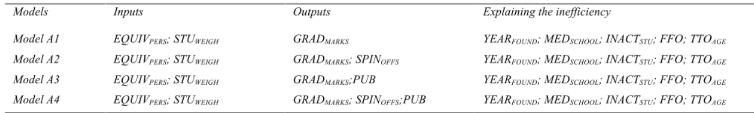
We start from the basic model (Model A1, Table 5) where equivalent personnel (EQUIVPERS) and the total weighted number of students (STUWEIGH) are used as inputs, the number of graduates weighted by their degree marks (GRADMARKS) is used as output and year of foundation of the university (YEARFOUND), the presence of a medical school (MEDSCHOOL), the age of the technology transfer offices (TTOAGE), the percentage of dropouts by the end of the 1st year (INACTSTU) and the ordinary financing fund received by the central government (FFO) are used in the variance of the efficiency. Keeping constant the input side and well the exogenous variables in the variance of the inefficiency, we explore whether the efficiency estimates change when additional outputs are considered. We first consider the number of graduates weighted by their degree marks (GRADMARKS) and the number of spin-off (SPINOFFS) as outputs (Model A2, Table 5), then the number of graduates weighted by their degree marks (GRADMARKS) and the number of publications (PUB) as outputs (Model A3, Table 5); finally, the last model (see Model A4, Table 5) includes all the three missions of the universities such as teaching, research and knowledge transfer, by using as outputs the number of graduates weighted by their degree marks (GRADMARKS), the number of spin-off (SPINOFFS) and the number of publications (PUB). See Table 5 below for a description of the variables used in the production set.
[Table 5 around here]
3.3. DATA
The dataset refers to 53 Italian public universities from 2006 to 2012. Variables included in the production set of the universities, such as EQUIVPERS, STUDWEIGH, GRADMARKS, , YEARFUND, MEDSCHOOL, INACTSTU, and FFO have been collected from the National Committee for the Evaluation of the University System (CNVSU) website23. SPINOFFS as well as TTO have been obtained from NETVAL which is the Italian association for the valorisation of results from public research. PUB were extracted from Thomson Reuters’ ISI Web of Science database, (being a part of the ISI Web of
23Http://www.cnvsu.it. Specifically, data have been collected by the Italian Ministry of Education, Universities and Research Statistical Office.
Knowledge) which lists publications from quality journals in all scientific fields; we count all publications (scientific articles, proceedings papers, meeting abstracts, reviews, letters, notes etc.) published in year, with at least one author declaring as an affiliate institution the HEI under consideration. Finally, the environmental variables used in order to estimate the local economic impact of HEIs, such as GDPC, LF, LG, are, instead, taken from the Italian National Institute of Statistics (ISTAT) website24.
4. THE EMPIRICAL EVIDENCE
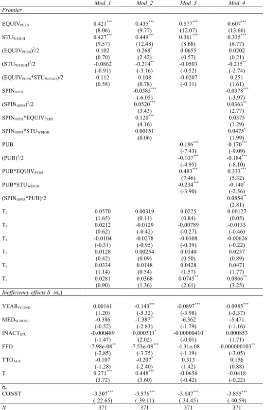
The estimated parameters of the stochastic education distance frontier, are presented in the Table 625. From a methodological perspective, the null hypothesis that there is no heteroscedasticity in the error term has been tested and rejected, at 1% significance level, using a Likelihood Ratio Test (LR), giving credit to the use of some exogenous variables, according to which the inefficiency term is allowed to change. In other words, the validity of heteroscedastic assumption has been confirmed, leading to the significance of the inefficiency term. The coefficients show that all the input variables have a positive and statistically significant effect on the various outcomes of the universities; the value of such coefficients are quite stable across all the specifications
[Table 6 around here]
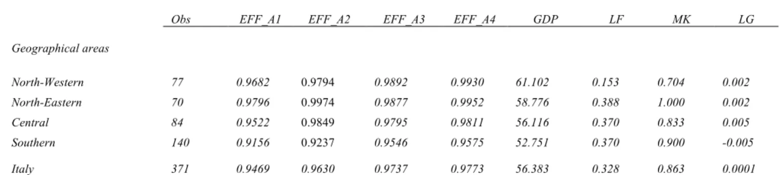
When looking at the (average) technical efficiency scores by geographical area (see Table 1 above) 26, the estimates reveal that institutions in the Central-North area (North-Western, North-Eastern and Central) outperform those in the Southern area; this result is consistent with previous evidence, as for instance that reported by Agasisti and Dal Bianco (2009), Agasisti, Barra and Zotti (2016) and Barra and Zotti (2016).
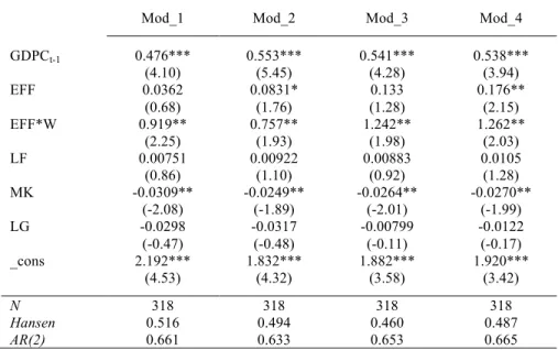
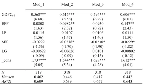
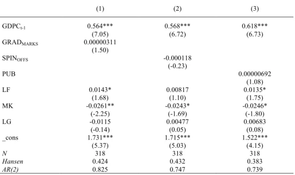
The GMM estimates of the growth model are presented in Table 7. The Arellano-Bond test results vouch for the appropriateness of the 2nd-order autoregressive specification while the Sargan tests are always insignificant validating the validity of the instruments and thus the correctness of the model. The lagged value of GDP per capita (GDPC) has a significant coefficient with positive sign in all models.
Moreover, the estimates suggest that the efficiency of universities (EFF) has a positive and significant effect on local growth. An increase by 1 percent in technical efficiency of universities increases the local growth by about 0.090 percent (see Table 7, Models 1-3) and by about 0.15 percent (see Table 7, Model 4). In other words, we find evidence that the presence of more efficient universities fosters local economic growth. Interestingly, the measure of the university efficiency become statistically significant both when reflects the teaching and the knowledge transfer mission on the universities (Mod_2, Tab. 7) and when all the three missions of the universities have been taken into account such as the teaching, research and knowledge transfer (Mod_4, Table 7). This result confirms the importance of knowledge spillovers from universities leading to regional wealth and competitiveness (Act et al. 2013; Ghio et al. 2015).
24Http://www3.istat.it/salastampa/comunicati/non_calendario/20050721_00/.
25We rely on the routines provided in STATA software (version 12) by Wang and Ho (2010) in order to make a within transformation to data using the “sf_fixeff” command.
26 Due to space constraint, the efficiency estimates are presented by geographical areas and on average over the period 2003-2011.
Estimates for each year and for each university are available on request.
This version is a draft. Please DO NOT QUOTE without the authors’ permission
To take into account whether the environment plays a role, we control for a measure of the state of the job market (LG), a measure of labor-force quality (LF) and for a measure of the concentration of the universities (MK). It is particularly interesting the negative and significant coefficient we found on the market share variable, meaning that the higher is the concentration of the universities the lower is the local growth. In other words, we found evidence that productivity gains are larger in areas where there is more competition between universities. This finding suggests that differences in local economic development might be due to the market structure of higher education, in the direction that a more competitive environment could lead to a higher human capital creation which in turn might imply a higher growth of the economy; thus, multiple HEIs located in the same region, or HEI effects spilling across regions, could be seen as competition leading to greater efficiency and student choice (i.e. for example stimulating the students’ freedom of choice through additional grants, loans and vouchers). Moreover, another explanation is that close proximity of multiple institutions permit collaboration, sharing of resources, greater division of production of qualified labor according to desired knowledge and skill sets, and thus have a positive impact on economic development. Both views provide a clue towards the expansion of pro-competitive policies in the Italian higher education sector (see Barra and Zotti, 2016).
[Table 7 around here]
4.1. A SPATIALLY WEIGHTED UNIVERSITY EFFICIENCY AND LOCAL GROWTH
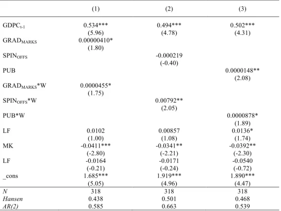
We extend the analysis to address potential geographical spillovers, considering the effects of the presence of higher education institutions on local economic development (results are shown in Table 8). We consider a measure of spatial dependence such as Efficiency * Spatial (EFF * W), being a spatially lagged regressor which measures whether the average productivity of labour is higher for those areas closer to the most efficient universities.
First of all, when we introduce the specification of the spatially weighted regressors27, the efficiency estimates do not change and remain statistically significant, particularly when models 2 and 4 are taken into account. Not only the introduction of the spatial effects does not alter our previous results, but we also find a significant and statistically positive effect of the spatially weighted variables. More precisely, when the specification of the spatially weighted efficiency of the university has been included (see Table 8), we find evidence that the average productivity of labour is higher in areas that are supported by the presence of universities which well-contribute with their missions; this suggests the presence of knowledge spillovers within areas having virtuous institutions. Again this is particularly true when the efficiency of the universities has been calculated taking into account considering the whole set of activities such as teaching, research and third mission. Indeed, the average productivity of labour in areas that are supported by the presence of universities which contribute well through the supply of high level human capital and the ability of transforming knowledge into economically relevant products. This result is in line with the idea that knowledge flows decrease as the geographic distance between HEI’s and regions increases (Paci and Usai, 2009) and that knowledge spillovers take place within a restricted geographic range (Moreno et al. 2005).
27 As already specified in Section 3.1., we use an inverse distance weighed matrix. In order to check whether a different solution regarding the choice of the distance matrix could affect the results, we have also repeat the main analysis using two other different weighting matrices such as a squared inverse distance matrix (following again Andersson et al. 2004) and a binary matrix. We did not find any statistically significant difference in the results. Due to space constraints, results are not presented in the paper and are available upon request.