Game-theoretical and monetary payoffs in laboratory experiments
R´obert F. Vesztega,∗, Yukihiko Funakia
aWaseda University, School of Political Science and Economics, 1-6-1 Nishiwaseda, Shinjuku-ku, 169-8050 Tokyo, Japan
Abstract
Experimental research in economics relies on performance-dependent monetary incen- tives to implement game-theoretical games in the laboratory. While the set of players and the set of strategies are unambiguously defined and controlled by the experimenter, game-theoretical payoffs are typically either assumed to coincide with monetary pay- offs, or are estimated ex-post based on observed actions and some sort of hypothesized rational behavior. We follow a different path and discuss results from an experiment on simple 2-person games in which participants were repeatedly asked to report their ex- pectations on the opponent’s behavior and their own level of satisfaction for each pos- sible outcome of the game. This approach allows us to reflect on experimental method- ology by directly comparing monetary incentives with (perceived) game-theoretical payoffs. We find that although repetition and experience help, they are unable to com- pletely align payoffs with monetary incentives. We also find that most participants seek to maximize money earnings in the experimental laboratory and they tend to perceive the games in the intended way. But at the same time, a small - yet non-negligible - fraction of the subject pool consistently interprets the game and, therefore, acts in an unexpected way.
Keywords: experimental method, induced-value method, prisoners’ dilemma, rationality
∗Corresponding author
Email addresses:rveszteg@aoni.waseda.jp(R´obert F. Veszteg),funaki@waseda.jp (Yukihiko Funaki)
“It is in fact very difficult to know what motivates subjects in a laboratory for experimentation in economics.” (Hausman, 2005)
1. Introduction
Ever since its early years experimental economics has been relying on the induced- value method (Smith, 1976) without explicitly questioning or studying its properties and its adequateness. When using the induced-value method, experimenters intend to achieve control by overwriting participants’ home-grown preferences with the help of monetary payoffs. In other words, when testing game theory in the experimental laboratory, researchers rely on thestandard payoff-bridging principleand assume that monetary payoffs correspond to game-theoretical payoffs. Although this assumption typically stays implicit and often outside the scope of the subsequent empirical and the- oretical analysis, it is – always and inevitably – jointly tested as an auxiliary hypothesis along with the main research hypotheses. This uncomfortable fact is an incidence of theDuhem-Quine problem that affects empirical science in general (Bardsley et al., 2010).1
For the sake of clarity, it is convenient to clarify our terminology right at the begin- ning: we refer to experimental incentives bymonetary payoffs,monetary incentives, orearnings, and to experimental incentives combined with personal motivations to- gether asgame-theoretical payoffs,satisfaction, orutility. This is in line with the stan- dard game-theoretical definition of payoffs which drive players’ choices and therefore should reflect everything that is relevant for players.
One way to affront the Duhem-Quine problem that arises around payoffs is to re- duce the gap between game-theoretical and monetary payoffs. In order to achieve that, Smith (1982) lists a number of characteristics that the appropriate reward scheme must have. He calls themnon-satiation, saliency,dominanceandprivacy. Without going into the details, all of them refer to the appropriate monetary incentives as part of thestandard payoff-bridging principle. Binmore (2007) follows a similar path, but includes two additional concerns on the list. Apart from the adequate (monetary) in- centives, he argues that the problem at participants’ hand should not be too complex, and they should have enough time for trial-and-error learning for game theory to work in the experimental laboratory.
1This introduction and the motivation behind our research largely build on chapters 3 and 6 from Bardsley et al. (2010), a unique book that takes a close look at the experimental method typically applied by economist and its long-ignored fundamental methodological issues.
An important stream of the behavioral economics literature surveyed by Camerer (2003) has also touched upon this problem and has introduced the concept ofother- regarding preferencesto cover the gap between earnings and utility. There is no final consensus as for the precise nature of these preferences which therefore appear under different names in the literature. The most prominent ones areregret theory(Loomes and Sugden, 1982),reciprocity theory(Rabin, 1993) and thetheory of inequity aversion (Fehr and Schmidt, 1999). While these theories propose different forms for the utility function that is meant to represent the underlying other-regarding preferences, they derive their conclusions in technically similar ways. First, experimental subjects are shown the game-theoretical payoffs in the game to be analyzed – typically expressed in so-called experimental monetary units (EMU) – and are explained how those are going to be transformed into real monetary payoffs at the end of the experiment based on a simple linear conversion rule (e.g.,1EMU =1USD). Second, the experimenter uses econometrics to estimate a utility function that best fits the observations on participants’
choices and behavior. This step relies on numerous assumptions. Beside the ones that are necessary to apply the chosen econometric model, the experimenter needs to believe that her subjects understood the rules of the game (including the available strategies, possible outcomes and corresponding theoretical payoffs) and they were acting in a way that can be mathematically described by maximizing a utility function. We will be referring to the latter assumption byrationality.
Our approach consists in checking whether the intended game has been imple- mented correctly by directly asking participants about their perception. The advantage of this approach is that we do not need to assume rationality behind the observations, however it comes at the price of having to rely on unincentivized answers to questions about personal satisfaction. In other words, we ask our subjects directly to report the game-theoretical payoffs they consider before making a decision. Although it is not the standard – or often required – experimental approach in economics, it has traces in the economics literature (Weibull, 2004; Guala, 2006) and it is a widely accepted practice by psychologists and political scientists (Dickson, 2011).
2. Experimental design
We conducted 10 experimental sessions using z-Tree (Fischbacher, 2007) at Waseda University (Tokyo, Japan) with altogether 200 students whom we recruited online. At the beginning of each session, printed instructions were given to participants and were read aloud by a computer software to the entire room. These instructions explained how individual choices and interaction among participants would determine mone-
tary payoffs that were received at the end of the session. Instructions were written in Japanese, presented sample screens to illustrate how the program works and con- tained some simple test questions whose answers were explained by the experimenter once all participants considered them.
We started our project by looking at “the most famous of all toy games” (Binmore, 2007), the prisoners’ dilemma game. We organized 3 treatments through 6 sessions (2 sessions dedicated entirely to each) that differed only in the name of the two available strategies:strategy A/strategy Bin the neutral treatment,cooperate/do not cooperate in the first framed treatment, andcooperate/betrayin the second framed treatment.
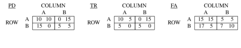
We did not find any significant and substantial difference in behavior or reported satis- faction levels among these 6 treatment, therefore we decided to pool the collected data for the sake of the statistical analysis. We complemented the 6 sessions of the pris- oners’ dilemma game (PD) with 2 sessions of a simultaneous-move binary trust game (TR) in the usual framing (send EMUs/keep EMUs), and with 2 sessions of another 2×2 matrix game that we call the favor game (FA) in a neutralstrategy A /strat- egy Bframing.2 Table 1 shows the payoff tables of our games. For simplicity, in this paper, we will be using the neutral way to refer to strategies: the first row/column is the cooperativestrategy A, while the second row/column is the competitivestrategy B.
Each game has a unique Nash equilibrium in pure strategies,{strategy B,strategy B}, which involves strictly dominant strategies for both players in PD, a weakly domi- nant strategy for the column player in TR, and a strictly dominant strategy for the row player in FA.3Also note that all of these Nash equilibria are Pareto dominated and the {strategy A,strategy A}profile would deliver the efficient outcome in each game.
Table 1: The analyzed games in normal form.
PD COLUMN
A B
ROW A 10 10 0 15
B 15 0 5 5
TR COLUMN
A B
ROW A 10 5 0 15
B 5 0 5 0
FA COLUMN
A B
ROW A 15 15 5 5
B 17 5 7 10
2If we had to tell an intuitive story around the FA game, we would refer to two people who work on a joint project, therefore share some common interest. The row player clearly has difficulties with meeting deadlines, while the column player can be on time, but would only make an effort if the row player made one, too. In other words, it is as if the column player asked a small but costly favor from the row player, and had to decide whether to really count on the row player’s contribution or not.
3The numbers in the payoff matrix that appeared on the screen during the experiments in the TR and FA games were 100-folds. The conversion rules between EMUs andUscaled final monetary gains to similar levels across the three games. For the sake of the exposition in this paper, we erased two zeros.
We implemented anonymous perfect-stranger matching in each session, i.e. par- ticipants were not informed about who their opponent was, and they were explained that the pairs would change randomly throughout the session without the chance of re- peating partner. Participants were not allowed to communicate with each other (other than choosing strategies and interacting through z-Tree). Each session consisted of 19 rounds of interaction among the 20 participants in groups of 2, with row-column roles being randomly reassigned by the computer in each round.
In each repetition, before required to make a strategic decision, participants were asked to indicate their satisfaction level in each of the four possible outcomes of the game by choosing an integer from 0 (least satisfied) to 10 (most satisfied).4 Similarly, participants were asked to state their beliefs as for the opponent choosing the coopera- tive strategy on a scale from 0% to 100% with 10% intervals. None of these questions were monetarily incentivized. While the latter question allows for such an incentiviza- tion – and experimental economists are typically expected to use it by a profession that is very much keen on monetary incentives –, the former questions do not. Mostly in order to keep the design simple, but also to avoid the documented hedging problems caused by incentivized belief elicitation techniques (Blanco et al., 2008), we decided to rely on participants’ intrinsic motivation and honesty in the answers to these ques- tions. As we later will discuss, in spite of the lack of monetary incentives, participants’
expectations about their opponent’s behavior were remarkably accurate.
After the last repetition of the game, participants answered a list of questions related to demographics, educational background and some questions on trust and cooperation inspired by the World Value Survey. A sample of the instructions and the questionnaire can be found in AppendixA.
At the end of the session, participants were paid individually and confidentially.
The individual monetary payoff for the session was computed as the sum of a 500U show-up fee and the converted accumulated payoffs over the 19 game repetitions. On average, it amounted to 1537U in the PD game, to 1173U in the TR game, and to 1419Uin the FA game (including the show-up fee). Each session lasted for about an hour, including instructions, questionnaires and payment.
4The Japanese keyword in these questions referring to personal satisfaction was “manzoku”. It is the standard equivalent of the English term, and dictionaries would typically translate it as “satisfaction”, “grat- ification”, or “content”.
3. Results
Our database contains observations for three types of variables. Firstly, we have a record of each participant’s choice over 19 repetition of the same game in possi- bly changing roles. Secondly, we have demographic information and data on gen- eral attitudes towards cooperations for each participant which stem from a short post- experimental questionnaire. Thirdly, we have participants’ self-declared satisfaction level for each possible outcome of the game on a common 0-to-10 integer scale, and their expectation as for the opponent’s behavior on a 0%-to-100% scale with 10% in- tervals. With the help of these observations, our objective is to compare the original game-theoretical games to the implemented ones, and to study how participants make their decisions, i.e. whether they are guided by game-theoretical payoffs or by mone- tary ones only.
In what follows, all statements related to statistical comparisons are based on for- mal parametric tests and the reported differences are to be interpreted as significantly different from 0 at 5% significance level, unless stated otherwise. The part of our anal- ysis that is concerned with time trends looks at four period blocks (first 5, second 5, third 5, and last 4 periods) instead of the 19 repetitions of the game separately.
Result 1. The ranking of outcomes based on game-theoretical and the ranking of out- comes based monetary payoff can differ in important ways. Therefore, the implemented game can be qualitatively different from the original game-theoretical one.
Given that individual satisfaction levels have no natural measurement unit, we re- quired participants to report their personal preferences with the help of a simple 0-to-10 integer scale. We expected (but did not instruct) them to assign 0 to the least desired outcome, 10 to the most desired one and rate the other two somewhere in the middle, because this is what introductory textbook on utility representation typically suggest.
It turns out that participants did so in only 63% of all cases, and avoided one or both of the extreme values in the rest. They assigned 0.6 on average to the least desired outcome and 9.6 on average to the most desired one.5 The subsequent analysis on indi- vidual decisions and individual perception of the game is based on modified individual scales. For the sake of comparing (average) game-theoretical payoffs with monetary payoffs across participants we rescaled the satisfaction reports before taking averages with the help of the following formula:vi =max10·(ui−minjuj)
juj−minjuj, whereuiis the reported
5This pattern did not change over time and the reported averages for each of the two extreme outcomes are identical up to one-digit precision in the four period blocks.
satisfaction level for outcomei.6
FIGURE 1 AROUND HERE
Figure 1: Average declared personal satisfaction levels after rescaling based on a 0 (least satisfied) - 10 (most satisfied) integer scale for each possible outcome, role, game, and period block. The grey areas represent the 95% confidence intervals around the point estimates. The (monetary) payoff vectors in the legend boxes list own payoffs in the first and the opponent’s payoffs in the second place. Nash-equilibrium payoff vectors are marked with∗.
The five graphs in figure 1 show the average (rescaled) declared, i.e. game-theoretical, payoffs for outcomes in each game, role and time block separately.7 The shaded grey areas around the averages represent the 95% confidence intervals. Those intervals are thinner for the PD game, because they have been computed with the help of consider- ably more observations than for the other games.
We wish to emphasize the following anomalies, or important differences, between game-theoretical and monetary payoffs.
1. Experimental participants may judge two different monetary payoffs as equal.
It is the case in the PD game between 10 and 15 that shows that there is no real temptation for prisoners to confess (i.e., to choosestrategy B). Therefore, behavior seems to be driven primarily by the fear of being taken advantage of.
Similarly, column players (i.e. trustees) in the TR game claim that collecting 5 or 15 monetary payoff units in the game are essentially the same. In other words, they are not strongly tempted to keep all the money (i.e., to fail to reciprocate and to choosestrategy B).
This type of anomaly made various experimenters suggest that players consider the entire monetary payoff vector instead of only one (albeit the only game- theoretically important one) of its components. After adjusting their free pa- rameters, models of other-regarding preferences (Camerer, 2003) can deliver in- difference between the above-mentioned pairs of earning vectors: (10; 10)and (15; 0), and(5; 10)and(15; 0).
2. Experimental participant may judge two equal monetary payoffs as different. It is the case for row players (i.e. trusters) in the TR game who, on average, be-
6For simplicity, we do not use any sub- or superindex denoting the participant, the game and the period, but the above transformation was carried out separately for each participants in each game in each period.
7The figure and our conclusions would not change qualitatively if we were to analyse the declared payoffs without rescaling.
lieve that it is strictly better to earn 5 monetary units when the opponent plays the cooperative strategy (i.e., reciprocates by choosingstrategy A) than to earn the same amount when the opponent chooses not to cooperate (i.e., fails to recip- rocate and choosesstrategy B). A similar pattern shows up for column players in the FA game, although the difference is not significant in the second period block. In that case, participants believe that it is strictly better to earn 5 mone- tary units by playing the cooperative strategy (strategy A) than to earn the same amount by choosing not to cooperate (strategy B).
The latter case – with(5; 5)and(5; 17)– constitutes an anomaly that models of other-regarding preferences are able to eliminate by incorporating the opponent’s earnings in the personal utility level. The former case, however, is a much harder nut as the two earning vectors deemed to be different in terms of satisfaction are exactly the same:(5; 0). Moreover the same two earning vectors are claimed to be equally satisfactory by players in the other role of the game.
3. Experimental participants may judge a larger monetary payoff as less desirable than a smaller one. This unusual effect appears in a weak form for row players in the FA game where the reported difference is significant at the 5% level in period blocks 1 and 3 only. In those cases, participants believe that it is better to earn 15 monetary units than 17.
Although the two rankings based on game-theoretical and monetary payoff are the same except for the above reported anomalies, those anomalies are enough to trigger unexpected behavior when the experimenter’s predictions are formed by looking at monetary payoff. It is also important to point out that the reported anomalies do not seem to become less frequent with time, i.e. with more experience or learning.
Figure 2 reveals the above described anomalies from a different – this time more individualistic – angle. The pie charts display five game types based on the 24 ways in which the four outcomes of our games could be ranked by participants according to some personal (week) preferences. Those implemented games that a participant described with a strict preferences ranking over outcomes are assigned to the corre- sponding unique category. For example, our category 1 (out of 24) collects games in which the first outcome is preferred to the second outcome, which in turn is preferred to the third outcome, which then in turn is preferred to the fourth outcome.8 Partici- pants were allowed to report indifferences (although they had to confirm those reports by affirmatively answering a yes-no type control question: “Are you sure you would
8We number the outcomes of the games from left to right and row by row starting at the top left corner.
like to report the same numbers for two or more outcomes?”). Reported indifferences make that a certain implemented game can fit into several categories. If, for example, a participant claims to be indifferent between the first and the second outcomes of the game, and also claims that both are strictly better than the third outcome which is then strictly preferred to the fourth one, the perceived game would fit into the previously described category 1, but also to the category that (weakly) ranks the second outcome as the best the first outcome as the second best, the third outcome as the third best and the fourth outcome as the fourth best. In such a case, we would assign the perceived game to both categories with weights12and12.9
The pies in figure 2 report the relative size of five game categories out of which one is the category of the intended, original game-theoretical game (based on monetary in- centives), while the other four are mutually exclusive categories that reflect the player’s best-response correspondence. In theA domcategory reported payoffs would suggest to playstrategy Aindependently of what the opponent is planning to do. TheB dom category is similar, but in those casestrategy Bshould be chosen without hesitation. In theassurancecategory, the player’s reported payoffs would guide him to try to match what the opponent is doing, i.e. playstrategy Aif the opponent playsstrategy A, and playstrategy Bif the opponent playsstrategy B. In thechickencategory players should try to avoid playing the strategy chosen by the opponent, i.e. they should playstrategy Aif the opponent playsstrategy B, and playstrategy Bif the opponent playsstrategy A.
The original games form a proper subset of one of these four categories given that, for example, they all have an inefficient Nash equilibrium. The PD game belongs to theB domcategory, the TR game for the row player toassurance, while for the column player toB dom, and the FA game for the row player toB dom, while for the column player toassurance. In order to make this slight abuse of labelling less confusing, the area that represents the correctly perceived games (always in green) and the area that represents the difference between the broader category and the category of correctly perceived games (e.g.B domfor the PD game) are labelled with their corresponding size in percentage terms. Furthermore, the outline color of the green area coincides with the area color of the broader category.
970% of all reports in the database show strict preferences. 22% of them include one indifference and the above-described categorization method assigns them to two categories (with weight12to each). 4%+4%=8%
include two indifferences and are assigned either to four categories (with weight14to each) if four outcomes are involved, or to six categories (with weight16 to each) if three outcomes are involved. A negligible 0.29%
(i.e., 11 reports in the database with 3800 observations) include three indifference and appear in all categories with the same weight (241).
FIGURE 2 AROUND HERE
Figure 2: Proportion of induced game types according to participants’ perception for each role and game (for all periods). The green areas represent the original game-theoretical game. The outline color of the green area indicates the broader game-type category. The categorization is based on weak preferences.
It is important to note that our analysis is one-sided, i.e. we look at games from the point of view of only one of the two players. Our five game categories are based on one’s best response correspondence and does take into consideration how the opponent perceives the game or how she is expected to perceive it. For example, the category assuranceis short foract as if you were participating in an assurance gameand not forassurance game.
The graphs in figure 2 are based on observations from all 19 rounds, but interest- ingly enough they would barely change when looking at the four period blocks sepa- rately, that is there does not seem to exist a learning process or any convergence towards the intended game-theoretical games. The main message from the figure is that the im- plementation rate of the theoretical game with the help of the induced-value method based on monetary incentives is roughly 40%-60%. In a non-negligible part of all cases (i.e., analyzed decision problems) the implemented game differs radically from the intended one. Dominant strategies might appear, disappear, or flip, and in general the perceived best-reponse correspondence might have an unexpected form.
If, instead of the above described (weak) one, we follow a strict approach and look at the correctly implemented (or perceived) games, the overall success rate of the value-induced method is 45%. In this case we require participants to report inequali- ties among payoffs in the correct directions and report indifference if and only if the corresponding monetary payoffs are equal. This result suggests, in other words, that it is in less than half of the cases true that participants rank the outcomes of the analyzed game strictly according to the monetary payoffs. When looking at different roles and games separately, the proportions differ in important ways. The highest success rate is the one in the PD game, 54%. The numbers are much lower in the TR (34% for the row player, 24% for the column player) and FA games (40% for the row player, 23%
for the column player).
Result 2. Participants report accurate expectations about the opponent’s behavior in spite of the absence of monetary incentives.
Figure 3 displays participants’ reported expectations and behavior, and has a simi-
lar structure to figure 1. As a general observation, even if it does not come as a surprise, we would like to emphasize that participants’ behavior (at the aggregate level) is sig- nificantly different from the theoretical predictions based on monetary payoffs. The observed proportions of cooperative choices, i.e.strategy A, is strictly positive with no- ticeable differences across roles and games especially in the early period blocks. There is a clear negative time trend towards the theoretical prediction in the PD, TR-row, and FA-column blocks, while choices do not change significantly on average in the TR-column and FA-row blocks.
FIGURE 3 AROUND HERE
Figure 3: Average proportion ofstrategy Achoices (ch. A) and expectations about the opponent choosing strategy A(exp. A) based on a simple 0% - 100% scale with 10% jumps for each possible outcome, role, game, and period block. For the asymmetric games (TR and FA), graphs show the observed behavior in a role and expected behavior for participants in that role as declared by participants in the other role. The grey areas represent the 95% confidence intervals around the point estimates.
What is much more remarkable is the global accuracy (based on averages) of indi- vidual expectations as for the opponent’s behavior. We observe that, in spite of the lack of monetary incentives and the perfect-stranger matching in our experiments, partici- pants’ expectations capture the overall trend in behavior. In other words, expectations move along the observed behavior or converge to it. Participants typically overestimate the probability of their opponent choosing the cooperative action (strategy B), but they update their estimates and manage to form accurate predictions as time goes by. In order to facilitate the study of expectations and their comparison to observed behavior, the TR-row block (for example) if figure 3 shows the row players’ decisions in the TR game and the column players’ reported expectations as for the row players’ behavior.
In what follows, we look at individual choices and the motivation behind them.
Unlike the usual approach, our analysis does not have to assume rationality behind participants’ choices, by which we refer to some sort of maximizing behavior, in oder to estimate the underlying motives. Our dataset contains direct observations on the most likely motives, i.e. monetary payoffs and personal satisfaction levels, and also participants’ self-declared main motive. Therefore, we are able to perform a different exercise and check how closely and consistently participants follow them.
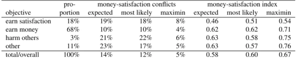
Result 3. Participants have an objective when participating in laboratory experiments and they follow it in a consistent way. Most of them act in order to maximize monetary gains, however almost a fifth of the subject pool do so to maximize satisfaction.
As displayed in first numerical column in table 2, in the post-experimental ques- tionnaire 68% of the participants claimed to have made their choices during the session with the objective of earning money, i.e. maximizing monetary payoffs. A considerable 18% declared the objective to be to earn, i.e. maximize, satisfaction. Interestingly, 3%
confessed to have been guided by the objective of harming others in the experiments, while 11% had some other, unspecified, goal.10 These numbers carry another mixed message for the experimental method which typically relies on monetary incentives and therefore implicitly assumes that participants come for money to the laboratory and they make their best when choosing their actions to earn as much of it as possible.
While this assumption seems to be correct for most participants, it is incorrect for a non-negligible part of the subject pool.
Table 2: Participants’ self-declared and observed objectives
pro- money-satisfaction conflicts money-satisfaction index objective portion expected most likely maximin expected most likely maximin
earn satisfaction 18% 19% 18% 8% 0.46 0.51 0.54
earn money 68% 10% 10% 4% 0.62 0.62 0.71
harm others 3% 21% 22% 6% 0.63 0.58 0.75
other 11% 23% 17% 5% 0.63 0.57 0.76
total/overall 100% 14% 12% 5% 0.58 0.60 0.67
NOTE. Expected: based on expected value computed with declared probabilities. Most likely: based on the opponent’s strategy that is declared to be expected with larger probability. Maximin: based on worst-case scenario. The money-satisfaction index
is 1 if all conflicts are resolved based on monetary payoffs; it is 0 if they are resolved based on game-theoretical payoffs.
Apart from the direct answers related to objectives in the questionnaire, partici- pants motivation can also be inferred with the help of their perception of the game and their behavior in it. Our database contains observations on 3420 decision situations out of which 462 (around 14%) constituted a clear conflict between monetary payoffs and game-theoretical payoffs to the participants. In those situations, the principles of expected-monetary-payoff maximization and expected-satisfaction maximization (both taking into consideration reported expectations on the opponent’s behavior) were giv- ing opposing indications whether the one or the other strategy should be chosen. Self- declared money-maximizers encountered the least number of such conflicts: in around 10% of all the decisions they faced. This proportion (displayed in the second numerical
10Saijo et al. (2012), using a completely different approach based on observed behavior and econometrics to elicit personal motivation, find that 74% of the subject pool belong to the “maximiser and reciprocator”
category. They also report that this result is not statistically different from the 86% that arises from partic- ipants’ answers in the post-experimental questionnaire. The equivalent number according to our categories would be the proportion of money-maximisers (68%) plus the proportion of satisfaction-maximizers (18%) that gives the exact same result of 86%.
column in table 2) is significantly and substantially smaller from the roughly 20% of conflicts that participants from the other self-declared categories experienced.
Although expected utility theory is a cornerstone of game theory, we have counted the conflicts based on other two decision criteria, too. The calculations behind themost likelycolumns in table 2 round the reported expectations to the closest extreme value of 0% or 100%, and compute a degenerate expected value for each strategy. When the opponent is expected to choose each strategy with 50% probability, we assume that the player attaches the largest attainable payoff number to each of his strategies.
This is a rather optimistic assumption on the opposite extreme from the assumption behind maximin strategies, but it is only required to break ties that constitute 7.5% of all reported expectations in the data. Themaximinapproach ignores reported expectations altogether and assigns to each strategy the smallest possible attainable payoff (with that particular strategy). Themost likelyresults are slightly, but not significantly different from the ones based expected values. Even the maximin column suggests that money- maximizer encounter half as many conflicts as satisfaction-maximizers. According to the latter column conflicts are less frequently which is due to the fact that participants tend to perceive the outcome with the lowest monetary payoff as the least desirable one in the analysed games. The subsequent analysis therefore focuses on conflicts and their resolution based on expected earnings and expected utility.
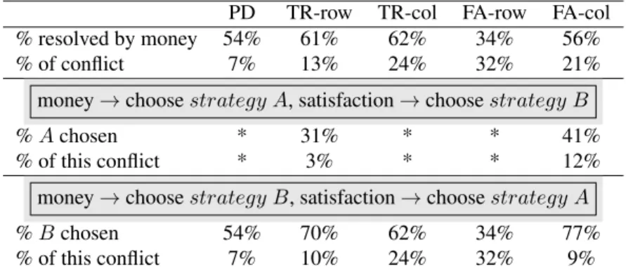
Different games and roles presented different degrees of conflict and predisposition to this problem. Table 3 shows the corresponding statistical results based on expected values. The least problematic decision to make was the one required in the PD game (7% of conflict), while the most problematic one was the the one row players were required to make in the FA game (32% of conflict).
Given the strategy chosen, we are able to infer how participants resolved conflicts, i.e. whether they let money or satisfaction to guide them. Unfortunately the numbers in table 3 do not give a crystal clear answer. Except for the row player’s problem in the FA game, conflicts are mostly resolved by looking at monetary payoffs. However these numbers are too close to 50% (between 54% and 62% in the first numerical row of table 3) to make a strong claim. It might be that the above numbers are aggregat- ing information on different types of participants. In line with this speculation, the last three columns in table 2 reveals that satisfaction-maximizing participants resolved conflicts by relying on what monetary payoffs suggest less frequently than all the other participants. We have created a simple numerical measure called money-satisfaction index which shows the fraction of conflicts resolved based on monetary payoffs.
When it comes to expected earnings and expected utility, the corresponding num- bers are 46% of the cases for satisfaction-maximizers and around 63% of the cases for
others (table 2). Now this difference is not only statistically significant, but also con- stitutes an important difference in behavior among different types of participants. The other two approaches, i.e.most likelyandmaximin, allow for the same conclusion.
Table 3: Money vs. satisfaction in conflict by game type and player’s role (based on expected values)
PD TR-row TR-col FA-row FA-col
% resolved by money 54% 61% 62% 34% 56%
% of conflict 7% 13% 24% 32% 21%
money→choosestrategy A, satisfaction→choosestrategy B
%Achosen * 31% * * 41%
% of this conflict * 3% * * 12%
money→choosestrategy B, satisfaction→choosestrategy A
%Bchosen 54% 70% 62% 34% 77%
% of this conflict 7% 10% 24% 32% 9%
NOTE. *In these roles and games, based on monetary incentives,strategy Bis dominant.
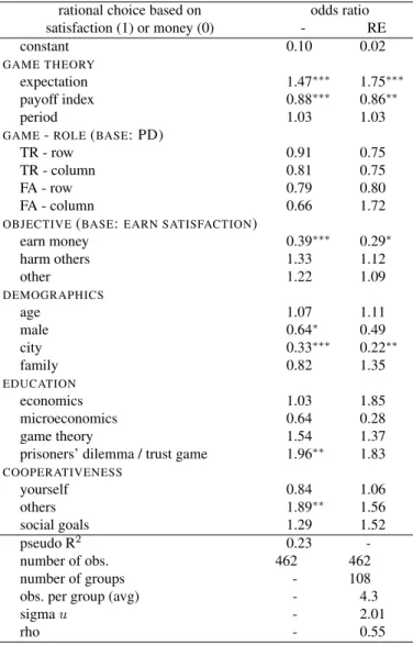
In order to further isolate the effects of the variables that might influence how par- ticipants choose between conflicting advices, we turn to regression analysis. Table 4 reports the odds ratios from two logistic regressions, one without and the other with random effects. The random effects we allow for are related to participants’ individual characteristics. We treat these effects as random rather than fixed, because our purpose is to study the larger population of potential experimental participants out of which we observed a random sample in the laboratory (Snijders, 2005). Our choice of the logit model over the probit is motivated by Wooldridge (2002) who points out (in chapter 15.8.3) that the unobserved-effect logit model has an important advantage over the pro- bit, because a consistent estimator can be obtained without any assumption about how the unobserved effects are related to the observed ones. We do not report marginal effects, but odds ratios based on coefficient estimates, as the fixed-effect specification makes the computation of the former impossible. The estimated odds ratios are the standard measure for the effect size for binary data (Ellis, 2010).
Our results suggest that participants resolve conflicts between monetary and game- theoretical incentives independently from the specific role and game, and also from the immediate experience (i.e., opportunity of learning proxied by theperiodvariable).11 Expectations concerning the opponent’s behavior are not only significant, but have an
11Refer to AppendixB for descriptive statistics on our variables.
important positive impact on leaning towards game-theoretical-payoff maximization.
Theexpectationvariable directly measures the expected probability of the opponent choosing the cooperative, and typically non-equilibrium,strategy A. For this very rea- son, we can reinterpret the variable as the expected probability of the opponent not being guided solely by monetary payoffs. In such a situation it could be reasonable to ignore the own incentives defined by monetary payoffs. Table 4 includes another highly significant, albeit less important, regressor calledpayoff indexwhich has a neg- ative effect on the odds of following game-theoretical payoffs. It is meant to compare the size (or strength) of monetary and game-theoretical payoffs, and is defined by the following formula:
payoff index= |Em(strategy A)−Em(strategy B)|
|Eu(strategy A)−Eu(strategy B)| ,
whereEudenotes expected utility, i.e. game-theoretical payoffs, andEmdenotes ex- pected monetary payoffs. The idea behind this variable is that participants compare the consequences of their choices both in terms of monetary gains and satisfaction levels.
When such a comparison leads to conflicting consequences, the absolute value (or size) of the additional gain drives behavior.
Apart from the regressors backed by game theory, a number of demographical vari- ables seem to have a significant impact on how participants solve the conflict between money and satisfaction maximization. While age and living with parents (versus living alone) does not matter, men tend to be guided more by monetary payoffs and so are participants from large cities.12
Education, in general, fails to have a significant impact on our dependent variable, but having heard about the game in question before (the prisoners’ dilemma in games PD and FA, and the trust game in game TR) matters in a positive way. This effect allows for two interpretations. On the one hand, we might say that thoseinformedparticipants know that the equilibrium outcome of the respective games is not efficient, and, in a rather naive way, they try to reach the efficient outcome. This is indeed a surprising result, because our regression controls for expectations and the relative size of the two types of incentives. On the other hand, we might look at this result as suggesting that informedparticipants know that game-theoretical payoffs do not only reflect monetary gains, and therefore they are much more likely to be guided by game-theoretical-payoff
12Ourcityvariable takes the value1if the participant is from one of the 10 major metropolitan areas in Japan. Those are: Tokyo, Nagoya, Osaka, Sapporo, Sendai, Yokohama, Kyoto, Kobe, Hiroshima, and Fukuoka.
maximization. Based on our questionnaire we are unable to tell these two explanations apart, however, the fact that thesocial goalvariable fails to have a significant impact makes us lean towards the second one. It is because, thesocial goalregressor controls for one’s belief whether it is cooperation or competition that helps to achieve social goals in general.
Between the variables that capture one’s cooperativeness and one’s beliefs on oth- ers’ cooperativeness, only the latter turns out to have a significant and sizable positive impact. We believe that this result is in line with our reinterpretation of the effect of theexpectationvariable. Whileexpectationrefers to the current anonymous opponent in the game,otherrefers to the broad society in general.
As for the self-reported objectives, those participants that have come to the lab- oratory for making money are more likely to follow monetary payoffs when making their decisions. The corresponding coefficient is not only highly significant, but shows that the odds of those participants considering the conflicting game-theoretical payoffs instead are 60% smaller (than the odds of participants who claim to have been guided by satisfaction levels). Although self-reported objectives do not perfectly explain the results of the individual decision-making process, the above statistical results shows a strong connection between them and proves the consistency claimed in result 3.
The random-effects model – which is reported in the last column in table 4 – allows for participant-specific differences and it is based on 108 groups, that is exactly the number of participants who ever experienced a conflict between monetary and game- theoretical incentives in our experiments. They did so in 4.3 occasions on average. The introduction of participant-specific random effects reduce the significance of several variables that represent personal characteristics, such as gender, having heard about the related game before, and personal beliefs about others’ cooperativeness. In the same fashion, also self-reported objectives turn out to be less significant in the model.
Although declaring money as the principal objective still has a sizable impact that is significant at the 10% level. In this model, it is the rho parameter that measures con- sistency in decision making as it pertains to a latent variable reflecting propensity to be guided by game-theoretical payoffs (as opposed to monetary payoffs). Its estimated value is 0.55 that is the correlation between this propensity in any two decision situa- tions with conflict for the same participant. In other words, 55% of the variance in the propensity to resolve conflict based on satisfaction levels can be attributed to personal characteristics.
Following Rodr´ıguez and Elo (2003), we estimated the correlation of this propen- sity in any two decision problems for a participant with a median linear predictor. The probability of resolving a conflicting decision problem in line with game-theoretical
Table 4: Resolution of the money-vs.-satisfaction conflict (logistic regressions without and with individual- specific random effects)
rational choice based on odds ratio
satisfaction (1) or money (0) - RE
constant 0.10 0.02
GAME THEORY
expectation 1.47∗∗∗ 1.75∗∗∗
payoff index 0.88∗∗∗ 0.86∗∗
period 1.03 1.03
GAME-ROLE(BASE: PD)
TR - row 0.91 0.75
TR - column 0.81 0.75
FA - row 0.79 0.80
FA - column 0.66 1.72
OBJECTIVE(BASE:EARN SATISFACTION)
earn money 0.39∗∗∗ 0.29∗
harm others 1.33 1.12
other 1.22 1.09
DEMOGRAPHICS
age 1.07 1.11
male 0.64∗ 0.49
city 0.33∗∗∗ 0.22∗∗
family 0.82 1.35
EDUCATION
economics 1.03 1.85
microeconomics 0.64 0.28
game theory 1.54 1.37
prisoners’ dilemma / trust game 1.96∗∗ 1.83
COOPERATIVENESS
yourself 0.84 1.06
others 1.89∗∗ 1.56
social goals 1.29 1.52
pseudo R2 0.23 -
number of obs. 462 462
number of groups - 108
obs. per group (avg) - 4.3
sigmau - 2.01
rho - 0.55
NOTE. Coefficient significantly different from zero at *10%, **5%, ***1%.
In case of indicator variables, the base or reference group is specified between parentheses above the block.
incentives is estimated to be of 45%, while the joint probability of the same solution in any two problems is 31%. It is much more than one would expect under independence across decision problems. This correlation is reflected in an odds ratio of 5.4, so for the participant at the median the odds of following game-theoretical payoffs are 5.4 times higher for those who have resolved another conflict in the same fashion than for those who didn’t.
We have shown so far that participants who show up in the experimental laboratory have well defined objectives that seem to guide their decisions in a consistent way.
Given the uncritical reliance of the experimental economics profession on monetary incentives, it seems that the group of money-maximizers constitutes the ideal subject pool for experimentation. The next and final test in our analysis is to take a closer look at this claim by checking the performance of the payoff bridging principle in inducing game-theoretical games in the laboratory.
Result 4. Participants who declare to have money-earning as their objective are more likely to perceive the game in the intended way, i.e. line with monetary incentives.
Table 5 displays the estimation results from a logistic regression without and with participant-related random effects whose dependent variable is a binary one indicating whether the participant perceives the game correctly, i.e. in line with monetary incen- tives, or not. It has been created following the strict-preference approach described earlier (see results 1). In this case all the 3420 observations, i.e. 19 decisions for each of the 180 participants, have been taken into consideration.
There seems to exist a significant, but negligible, learning process that works in favor of the value-induced method (period). Similarly, previous studies in Economics and Game Theory have a very important and highly significant impact on the odds of a correct perception of the game. Having studied the related game seems to reduce those odds. We can not but speculate again about the reasons behind this result. We be- lieve that it is probably, because the prisoners’ dilemma and the trust game are usually presented as puzzles in the classroom and the subsequent explanation typically empha- sizes the desirability of the efficient outcome as compared to the equilibrium outcome.
Similarly, seeing oneself and the others are cooperative reduces the odds of success of implementation in important ways. The large positive impact ofsocial goalsmay seem counterintuitive, however it is very much in line with the original theoretical consider- ations behind our games: for the efficient outcome it is necessary for both participants to cooperate.
Participants from large cities and those who live with their families seem to perceive the games differently. The former negative effect is puzzling, however it’s relatively
Table 5: Success of game implementation based on monetary incentives(logistic regressions without and with random effects)
perceived game is odds ratio
correct (1) or different (0) - RE
constant 1.46 0.75
GAME THEORY
period 1.02∗∗ 1.04∗∗∗
GAME-ROLE(BASE: PD)
TR - row 0.40∗∗∗ 0.21∗∗
TR - column 0.26∗∗∗ 0.06∗∗∗
FA - row 0.62∗∗∗ 0.36
FA - column 0.25∗∗∗ 0.07∗∗∗
OBJECTIVE(BASE:EARN SATISFACTION)
earn money 1.51∗∗∗ 2.88
harm others 0.73 0.49
other 0.40∗∗∗ 0.12∗∗
DEMOGRAPHICS
age 0.99 1.03
male 0.91 1.02
city 0.87∗ 0.55
family 0.60∗∗∗ 0.24∗∗
EDUCATION
economics 1.66∗∗∗ 3.22
microeconomics 0.82 0.80
game theory 1.57∗∗∗ 2.32
prisoners’ dilemma / trust game 0.79∗∗ 0.66
COOPERATIVENESS
yourself 0.77∗∗∗ 0.62
others 0.75∗∗∗ 0.41
social goals 1.22∗∗ 1.51
pseudo R2 0.10 -
number of obs. 3420 3420
number of groups - 180
obs. per group (avg) - 19.0
sigmau - 3.41
rho - 0.78
NOTE. Coefficient significantly different from zero at *10%, **5%, ***1%.
In case of indicator variables, the base or reference group is specified between parentheses above the block.
small size and large p-value make it less so.
The main message for the experimental economist from table 5, apart from the rather slow learning process, is that the success of implementation differs in important ways across different games. The related questions lie aside from the main purpose of this paper, nevertheless it would be important to understand whether games with dominant strategies, games with symmetric payoff structure, etc. are more or less easy to implement in the laboratory. As for participants self-declared objective, the odds of correctly perceiving the game is 51% larger for money maximizers than for peo- ple whose objective is gaining satisfaction. Theothercategory probably groups those people who did not have a precise objective and/or were confused during the experi- ment. They constitute 11% of all analyzed decisions, which is fortunately a small, but non-negligible proportion.
In the random-effect model rho is 0.78, i.e. 78% of the variance in success of imple- mentation in the experimental laboratory can be attributed to personal characteristics.
Evaluated at the median, the probability of perceiving the game correctly is 43%, while the joint probability of the same in any two decision problems is 33%. Again, it is much more than one would expect under independence across decision problems.
4. Conclusions
If we were to summarize the results of the paper in a short message, we would is- sue the following warning to experimental economists: “The standard payoff-bridging principle seems to work for a broad majority of participants in the laboratory, but it seems to fail in unpredictable ways for a non-negligible part of the subject pool.”
Subject pools in the experimental laboratory recruited in the usual ways (websites, campus-wide posters) are far from being random or representative even for the nar- rower student population, because participants self-select into laboratory. With the help of a large database containing information on numerous experimental sessions over several years, Guillen and Veszteg (2012) conclude that men and (in monetary terms) well-performing participants are more likely to come back and participate again in experiments.
This paper raises an other red flag by showing that participants arrive with different objectives to the laboratory that influence their decisions directly and also indirectly through intervening in the way they perceive the games under study. The usual mon- etary incentives built on the standard payoff-bridging principle (Smith, 1982) can not guarantee always the correct implementation of game-theoretical games in the experi-
mental laboratory.13 Apart from the confused and/or careless participants (in theother category) whose decisions compose 11% of our database and the rather peculiar group of participants whose self-declared objective was to hurt the opponent (3% of all en- tries in the dataset), an important 18% of the subject pool claim to have made their decisions with the goal of maximizing satisfaction level. It is the remaining 68% that correspond to the ideal participant who comes to earn money.
As for the conditions by Binmore (2007) under which one can reasonably expect game theory to work in the experimental laboratory, our experimental design contains only 19 repetition of the game (primarily because of our desire to employ perfect- stranger matching and the limited size of our laboratory) therefore we are unable to make strong claims related to learning on the perception of laboratory games. How- ever in line with Binmore (2007), we used very simple2×2matrix games (including the widely known simple prisoners’ dilemma game) and still evidenced differing im- plementation levels across games.
Now if one’s purpose is to test game theory in the laboratory and put theoretical predictions and laboratory observations side by side, we urge to double-check whether participants are considering the intended game or a completely different one before asking them to make a decision. We encourage experimental economists to use direct and possibly unincentivized questions to carry out those checks,. Those would also help to understand what really motivates participants in the laboratory.
We have shown that participants arrive with their objectives to the laboratory. It is only natural to ask whether they succeed in achieving them or not. Without going into the details, the overall results are as follows. Money-maximizers earned 1131Uon average over the 19 repetitions, slightly and insignificantly less than the satisfaction- maximizers who made 1192U.14 In terms of satisfaction levels, the overall average for the 19 outcomes that arose in the experimental session based on reports by money- maximizers was 4.36 (satisfaction points), significantly less than the 4.86 (satisfaction points) for satisfaction-maximizers (p-value=0.0007)15. Although not in a statistically significant way, participants whose self-declared objective was to hurt the opponent outperformed the other two categories by earning 1240Uand 5.13 satisfaction points
13By “usual” we not only refer to the standard payoff-bridging principle in general, but also to the typical magnitude of experimental earnings (around 1500Ufor a 90-minutes session in Tokyo) and the way they are defined and explained (through a linear rule stated in the instructions) in the experimental laboratory to participants.
14All monetary earning reported in the paragraph are net of the show-up fee.
15The satisfaction averages are based on reported satisfaction levels without rescaling or any other modi- fication.
on average.
[1] Bardsley, N., Cubitt, R., Loomes, G., Moffatt, P., Starmer C., Sugden, R.
(2010). Experimental economics: Rethinking the rules. Princeton University Press, Princeton, NJ.
[2] Binmore, K. (2007).Does game theory work? The bargaining Challenge. MIT Press, Cambridge, MA.
[3] Blanco, M., Engelmann, D., Koch, A. K., Normann, H. T. (2010). Belief elicita- tion in experiments: is there a hedging problem?Experimental Economics, 13(4):
412-438.
[4] Camerer, C. F. (2003).Behavioral game theory: Experiments in strategic inter- action. Princeton University Press, Princeton, NJ.
[5] Dickson, E. S. (2011). Economics vs psychology experiments: Stylization, in- centives, and deception. In Cambridge handbook of experimental political sci- ence(eds. J. N. Druckman, D. P. Green, J. H. Kuklinski, A. Lupia). Cambridge University Press, New York, NY.
[6] Ellis, P. D. (2010). The essential guide to effect sizes: Statistical power, meta- analysis, and the interpretation of research results, Cambridge University Press.
[7] Fehr, E., Schmidt, K. M. (1999). A theory of fairness, competition, and coopera- tion.The Quarterly Journal of Economics, 114(3), 817–868.
[8] Fischbacher, U. (2007). z-Tree - Zurich toolbox for readymade economic experi- ments - Experimenter’s manual.Experimental Economics, 10(2), 171-178.
[9] Guala, F. (2006) Has game theory been refuted? Journal of Philosophy, 103(5), 239-63.
[10] Guillen, P., Veszteg, R. (2012). On “lab rats”.Journal of Socio-Economics, 41(5), 714-720.
[11] Hausman, D. M. (2005). ‘Testing’ game theory.Journal of Economic Methodol- ogy, 12(2): 211-23.
[12] Loomes, G., Sugden, R. (1982). Regret theory: An alternative theory of rational choice under uncertainty.The Economic Journal, 92(368), 805–824.
[13] Rabin, M. (1993). Incorporating fairness into game theory and economics.The American Economic Review, 83(5), 1281–1302.
[14] Rodr´ıguez, G., Elo, I. (2003) Intra-class correlation in random-effects models for binary data.The Stata Journal, 3(1), 32-46.
[15] Saijo, T., Okano, Y., Yamakawa, T. (2012) The approval mechanism experiment:
A solution to prisoner’s dilemma, mimeo.
[16] Smith, V. L. (1976). Experimental economics: Induced value theory.American Economic Review, 66(2), 274–279.
[17] Smith, V. L. (1982). Microeconomic systems as an experimental science.Ameri- can Economic Review, 72(5), 923-955.
[18] Snijders, T. A. B. (2005). Fixed and random effects. inEncyclopedia of statistics and behavioural science, Volume 2 (eds. B. S. Everitt, D. C. Howell). Wiley, Chicester.
[19] Weibull, J. (2004). Testing game theory. InAdvanced in understanding strategic behaviour(ed. S. Huck). Palgrave, New York, NY.
[20] Wooldridge, J. M. (2002).Econometric analysis of cross section and panel data, MIT Press.
AppendixA. Experimental instructions and questionnaire
This is the English translation of the instructions we used in the PD game. The other sessions we based on similar documents which are available from the authors upon request both in English and Japanese.
Prisoner’s dilemma game
Thank you for participating in this experiment. Before we start, we will read these instructions aloud and answer all the questions that arise.
In this experiment, you will be required to make a decision in 19 independent repe- titions of the same game. In each repetition, you will be randomly paired with an other participant. This means that you will be interacting with a different person in each round.
Both you and your opponent will have to choose a strategy simultaneously, i.e.
without exactly knowing what the other person is going to do. Depending on the strat- egy chosen by you and and by the other person, you will earn different amounts of money expressed in Experimental Monetary Units (EMU).
In each repetition of the game, both you and your opponent will have to choose be- tween “strategyA” and “strategyB”. Here is how your monetary gains are determined by your choice.
• If both of you choose “strategyA”, both of you will earn10EMU.
• If both of you choose “strategyB”, both of you will earn5EMU.
• If you choose“ strategyA” and your opponent chooses “strategyB”, you will earn0EMU and your opponent will earn15EMU.
• If you choose “strategyB” and your opponent chooses “strategyA”, you will earn15EMU and your opponent will earn0EMU.
The following table summarizes this information.
if your opponent chooses if your opponent chooses
“strategyA” “strategyB”
if you choose you earn 10EMU you earn 0EMU
“strategyA” your opponent earns 10EMU your opponent earns 15EMU
if you choose you earn 15EMU you earn 5EMU
“strategyB” your opponent earns 0EMU your opponent earns 5EMU
The amount of money (in Japanese yen) that you will be paid at the end of the experiment will be determined based on your aggregated total earning during the 19 repetitions of the game.1EMU will be exchanged for10Japanese yen.
During the experiment we will ask you several simple questions related to your decisions and your opinion about the game. The answer that you give will be treated confidentially, in particular, your opponent will not receive any information about them.
Please try to give as honest answers as possible.
Questionnaire
This is the list of questions that appeared on screen in the post-experimental ques- tionnaire.
• Please indicate your age.
• Please indicate your gender.
– male – female
• Please indicate your major.
• Have you ever studied Economics before?
– yes – no
• Have you ever studied Microeconomics before?
– yes – no
• Have you ever studied Game Theory before?
– yes – no
• Have you ever heard about the Prisoners’ Dilemma before?
– yes – no
• Is your hometown any of the following places? Tokyo, Nagoya, Osaka, Sapporo, Sendai, Yokohama, Kyoto, Kobe, Hiroshima, Fukuoka
– yes – no
• Do you live together with your family?
– yes – no
• As compared to the other participants, do you think you chose “strategy A” more often?
– I chose “strategy A” more often than others – I chose “strategy A” as often as others – I chose “strategy B” more often than others
• Do you consider yourself a cooperative person?
– yes – no
• Do you think most people are normally cooperative?
– yes – no
• Do you think it is cooperation or competition that is more important to achieve s social goal?
– cooperation – competition
• What was your objective when making your decisions during the experiment?
– maximize satisfaction – maximize monetary earnings – hurt the opponent
– other
AppendixB. Descriptive statistics
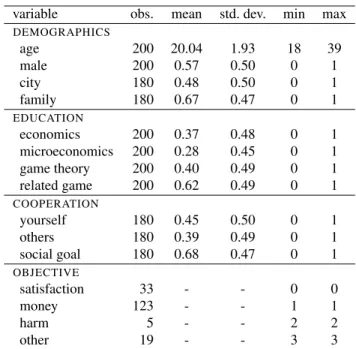
Table B.6: Descriptive statistics on items in the questionnaire
variable obs. mean std. dev. min max
DEMOGRAPHICS
age 200 20.04 1.93 18 39
male 200 0.57 0.50 0 1
city 180 0.48 0.50 0 1
family 180 0.67 0.47 0 1
EDUCATION
economics 200 0.37 0.48 0 1
microeconomics 200 0.28 0.45 0 1
game theory 200 0.40 0.49 0 1
related game 200 0.62 0.49 0 1
COOPERATION
yourself 180 0.45 0.50 0 1
others 180 0.39 0.49 0 1
social goal 180 0.68 0.47 0 1
OBJECTIVE
satisfaction 33 - - 0 0
money 123 - - 1 1
harm 5 - - 2 2
other 19 - - 3 3