Dual-Tone Multi-Frequency Dual-Tone Multi-Frequency Dual-Tone Multi-Frequency Dual-Tone Multi-Frequency Dual-Tone Multi-Frequency Coding Coding Coding
Coding Coding 14 14 14 14 14
441 441 441 441 441
14.1 14.1 14.1
14.1 14.1 INTRODUCTION INTRODUCTION INTRODUCTION INTRODUCTION INTRODUCTION
DTMF is the generic name for pushbutton telephone signaling equivalent to the Bell System’s TouchTone®. Dual-Tone Multi-Frequency (DTMF) signaling is quickly replacing dial-pulse signaling in telephone networks worldwide. In addition to telephone call signaling, DTMF is becoming popular in interactive control applications, such as telephone banking or electronic mail systems, in which the user can select options from a menu by sending DTMF signals from a telephone.
To generate (encode) a DTMF signal, the ADSP-2100 adds together two sinusoids, each created by software. For DTMF decoding, the ADSP-2100 looks for the presence of two sinusoids in the frequency domain using modified Goertzel algorithms. This chapter shows how to generate and decode DTMF signals in both single channel and multi-channel
environments. Realizable hardware is briefly mentioned.
DTMF signals are interfaced to the analog world via codec (coder/
decoder) chips or linear analog-to-digital (A/D) converters and digital-to- analog (D/A) converters. Codec chips contain all the necessary A/D, D/A, sampling and filtering circuitry for a bidirectional analog/digital interface. These codecs with on-chip filtering are sometimes called codec/
filter combo chips, or combo chips for short. They are referred to as codecs in this chapter.
The codec channel used in this example is bandlimited to pass only frequencies between 200Hz and 3400Hz. The codec also incorporates companding (audio compressing/expanding) circuitry for either of the two companding standards (A-law and µ-255 law). These two standards are explained in Chapter 11, Pulse Code Modulation. Companding is the process of logarithmically compressing a signal at the source and expanding it at the destination to maintain a high end-to-end dynamic range while reducing the dynamic range requirement within the communication channel.
In the example of DTMF signal generation shown in this chapter, the ADSP-2100 reads DTMF digits stored in data memory in a relocatable
14 14 14 14 14
442 442 442 442 442
Dual-Tone Multi-Frequency Dual-Tone Multi-Frequency Dual-Tone Multi-Frequency Dual-Tone Multi-Frequency Dual-Tone Multi-Frequency
look-up list. Alternatively, a DTMF keypad could be used for digit entry.
In either case, the resultant DTMF tones are generated mathematically and added together. The values are logarithmically compressed and passed to the codec chip for conversion to analog signals. Multi-channel DTMF signal generation is performed by simply time-multiplexing the processor among the channels.
On the receiving end, the ADSP-2100 reads the logarithmically compressed, digital data from the codec’s 8-bit parallel data bus,
logarithmically expands it to its 16-bit linear format, performs a Goertzel algorithm — a fast DFT (discrete Fourier transform) calculation — for each tone to detect, then passes the results through several tests to verify whether a valid DTMF digit was received. The result is coded and written to a memory-mapped I/O port. Multi-channel DTMF decoding is also performed by time-multiplexing the channels.
14.2 14.2 14.2 14.2
14.2 ADVANTAGES OF DIGITAL IMPLEMENTATION ADVANTAGES OF DIGITAL IMPLEMENTATION ADVANTAGES OF DIGITAL IMPLEMENTATION ADVANTAGES OF DIGITAL IMPLEMENTATION ADVANTAGES OF DIGITAL IMPLEMENTATION
Several chips are available which employ analog circuitry to generate and decode DTMF signals for a single channel. This function can be digitally implemented using the ADSP-2100. The advantages of a digital system include better accuracy, precision, stability, versatility, and
reprogrammability as well as lower chip count, and thereby reduced board-space requirements.
Table 14.1 compares the tone accuracy expected of a DTMF tone dialer chip with the accuracy of tones generated by the ADSP-2100. Note that a tone dialer chip is an application-specific device with preprogrammed frequencies for use on a single channel, whereas the ADSP-2100 is a general purpose microprocessor which can be programmed to generate any frequency for many separate channels. When using the ADSP-2100, the frequency values can be specified to within 16 bits of resolution, implying an accuracy of 0.003%.
By simply changing the frequency values, the ADSP-2100 tone generator can be fine-tuned or reprogrammed for other tone standards, such as CCITT 2-of-6 Multi-Frequency (MF), call progress tones, US Air Force 412L, and US Army TA-341/PT. Since the numbers stored in data memory do not change in value over time or temperature, the precision and
stability of a digital solution surpasses any analog equivalent. DTMF encoding and decoding can be written as a subfunction of a larger program, eliminating the need for separate components and specialized interface circuitry.
14 14 14 14 14 Dual-Tone Multi-Frequency
Dual-Tone Multi-Frequency Dual-Tone Multi-Frequency Dual-Tone Multi-Frequency Dual-Tone Multi-Frequency
443 443 443 443 443
DTMF Standard Typical frequency from Frequency from Frequency hybrid tone-dialer chip ADSP-2100 program
using 3.579545MHz crystal
% deviation % deviation
697.0Hz 699.1Hz +0.31% 697.0Hz ±0.003%
770.0Hz 766.2Hz –0.49% 770.0Hz ±0.003%
852.0Hz 847.4Hz –0.54% 852.0Hz ±0.003%
941.0Hz 948.0Hz +0.74% 941.0Hz ±0.003%
1209.0Hz 1215.9Hz +0.57% 1209.0Hz ±0.003%
1336.0Hz 1331.7Hz –0.32% 1336.0Hz ±0.003%
1477.0Hz 1471.9Hz –0.35% 1477.0Hz ±0.003%
1633.0Hz 1645.0Hz +0.73% 1633.0Hz ±0.003%
Table 14.1 Precision of Analog and Digital Tone Generation Table 14.1 Precision of Analog and Digital Tone Generation Table 14.1 Precision of Analog and Digital Tone Generation Table 14.1 Precision of Analog and Digital Tone Generation Table 14.1 Precision of Analog and Digital Tone Generation
14.3 14.3 14.3 14.3
14.3 DTMF STANDARDS DTMF STANDARDS DTMF STANDARDS DTMF STANDARDS DTMF STANDARDS
The DTMF tone signaling standard is also known as TouchTone or MFPB (Multi-Frequency, Push Button). TouchTone was developed by Bell Labs for use by AT&T in the American telephone network as an in-band signaling system to supersede the dial-pulse signaling standard. Each administration has defined its own DTMF specifications. They are all very similar to the CCITT standard, varying by small amounts in the
guardbands (tolerances) allowed in frequency, power, twist (power difference between the two tones) and talk-off (speech immunity). The CCITT standard appears as Recommendations Q.23 and Q.24 in Section 4.3 of the CCITT Red Book, Volume VI, Fascicle VI.1. Other standards (AT&T, CEPT, etc.) are listed in References, at the end of this chapter.
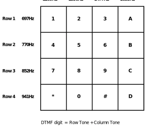
Two tones are used to generate a DTMF digit. One tone is chosen out of four row tones, and the other is chosen out of four column tones. Two of eight tones can be combined so as to generate sixteen different DTMF digits. Of the sixteen keys shown in Figure 14.1, on the next page, twelve are the familiar keys of a TouchTone keypad, and four (column 4) are reserved for future uses.
A 90-minute audio-cassette tape to test DTMF decoders is available from Mitel Semiconductor (part number CM7291). There also exists a standard describing requirements for systems which test DTMF systems. This standard is available from the IEEE as ANSI/IEEE Std. 752-1986.
14 14 14 14 14
444 444 444 444 444
Dual-Tone Multi-Frequency Dual-Tone Multi-Frequency Dual-Tone Multi-Frequency Dual-Tone Multi-Frequency Dual-Tone Multi-Frequency
Column 1 Column 2 Column 3 Column 4
Row 1
Row 2
Row 3
Row 4
1209Hz 1336Hz 1477Hz 1633Hz
697Hz
770Hz
852Hz
941Hz
1 2 3 A
4 5 6 B
7 8 9 C
* 0 # D
DTMF digit = Row Tone + Column Tone
Figure 14.1 DTMF Digits Figure 14.1 DTMF Digits Figure 14.1 DTMF Digits Figure 14.1 DTMF Digits Figure 14.1 DTMF Digits
14.4 14.4 14.4 14.4
14.4 DTMF DIGIT GENERATION PROGRAM DTMF DIGIT GENERATION PROGRAM DTMF DIGIT GENERATION PROGRAM DTMF DIGIT GENERATION PROGRAM DTMF DIGIT GENERATION PROGRAM
Generation of DTMF digits is relatively straightforward. Digital samples of two sine waves are generated (mathematically or by look-up tables), scaled and then added together. The sum is logarithmically compressed and sent to the codec for conversion into the analog domain.
A sine look-up table is not used in this example because the sine can be computed quickly without using the large amount of data memory a look- up table would require. The sine computation routine is efficient, using only five data memory locations and executing in 25 instruction cycles.
The routine used to compute the sine is from Chapter 4, Function Approximation. This routine evaluates the sine function to 16 significant bits using a fifth-order Taylor polynomial expansion. The sine
computation routine is called from the tone generation program as an external routine; refer to that chapter for details on the sine computation routine.
14 14 14 14 14 Dual-Tone Multi-Frequency
Dual-Tone Multi-Frequency Dual-Tone Multi-Frequency Dual-Tone Multi-Frequency Dual-Tone Multi-Frequency
445 445 445 445 445
To build a sine wave, the tone generation program utilizes two values.
One, called sum, keeps track of where the current sample is along the time axis, and the other, called advance, increments that value for the next sample. Since the DTMF tone generation program generates two tones, there are two different sum values and two different frequency values (stored in the variables hertz). The value sum is stored in data memory in a variable called sum. Sum is modified every time a new sample is
calculated. The value advance is calculated from a data memory variable called hertz. Hertz is a constant for a given tone frequency. The ADSP-2100 calculates the advance value from a stored hertz variable instead of storing advance as the data memory variable because this allows you to read the frequency being generated in Hz directly from the data memory display (in decimal mode) of the ADSP-2100 Simulator or Emulator.
The sum values are dm(sin1) and dm(sin2) in Listing 14.1 (see Program Listings at the end of this chapter). The advance values are derived from the variables dm(hertz1) and dm(hertz2) in Listing 14.1. For readable source code and easy debugging, Listing 14.1 uses two data memory variables dm(sin1) and dm(sin2) to store the value returned from each call to the sine subroutine rather than storing the value in a register. These variables are then added together, resulting in a DTMF output signal value.
The sampling frequency of telephone systems is 8kHz. Therefore, the ADSP-2100 must output samples every 125µs. An 8kHz TTL square wave is applied to an interrupt (IRQ3 in this case) pin of the ADSP-2100. The ADSP-2100 is initialized for edge-sensitive interrupts with interrupt- nesting mode disabled (see Listing 14.1, two lines immediately preceding the label wait_int near the top of executable code). The sampling
frequency, in conjunction with the advance value, determines the frequency of the sine wave generated.
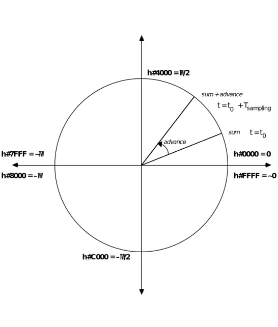
Circular movement around a unit circle is analogous to linear motion along the time axis of a sine wave, one revolution of the circle
corresponding to one period of the wave. The range of inputs to the sine function approximation subroutine is –π to 0 to +π radians. This range maps to the 16-bit hexadecimal numbers H#8000 to H#FFFF and H#0000 to H#7FFF (see Figure 14.2 on the next page and Table 14.2 following it).
All of the 16-bit numbers are equally spaced around the unit circle, dividing it into 65536 parts. The advance value is added to the sum value during each interrupt. To generate a 4kHz sine wave, the advance value would have to be 32768, equivalent to π radians, or a jump halfway around the unit circle. Because Nyquist theory dictates that 4kHz is the highest frequency that can be represented in an 8kHz sampling-frequency
14 14 14 14 14
446 446 446 446 446
Dual-Tone Multi-Frequency Dual-Tone Multi-Frequency Dual-Tone Multi-Frequency Dual-Tone Multi-Frequency Dual-Tone Multi-Frequency
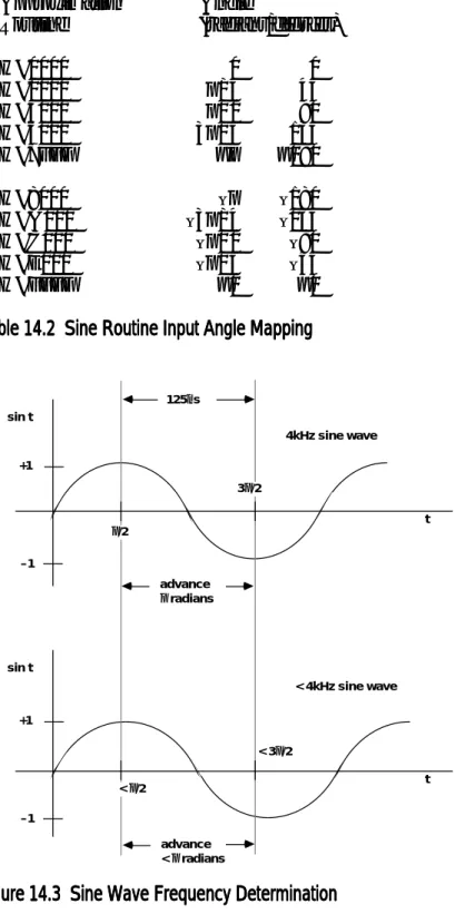
system, this is the maximum advance value that can be used. For a sine wave frequency of less than 4kHz, the advance value would be
proportionally less (see Figure 14.3).
Figure 14.2 Sine Routine Input Angle Mapping Figure 14.2 Sine Routine Input Angle Mapping Figure 14.2 Sine Routine Input Angle Mapping Figure 14.2 Sine Routine Input Angle Mapping Figure 14.2 Sine Routine Input Angle Mapping
advance value = 65536 sampling frequency tone frequency desired
advance
h#0000 = 0 h#FFFF = ~0 h#4000 = π/2
h#C000 = –π/2 h#7FFF = ~π
h#8000 = –π
sum + advance
sum
t = t + Tsampling
0
t = t0
14 14 14 14 14 Dual-Tone Multi-Frequency
Dual-Tone Multi-Frequency Dual-Tone Multi-Frequency Dual-Tone Multi-Frequency Dual-Tone Multi-Frequency
447 447 447 447 447
Input to Sine Equivalent Input Approximation Angle
Routine (radians/degrees)
H#0000 0 0
H#2000 π/4 45
H#4000 π/2 90
H#6000 3π/4 135
H#7FFF ~π ~180
H#8000 –π –180
H#A000 –3π/4 –135
H#C000 –π/2 –90
H#E000 –π/4 –45
H#FFFF ~0 ~0
Table 14.2 Sine Routine Input Angle Mapping Table 14.2 Sine Routine Input Angle Mapping Table 14.2 Sine Routine Input Angle Mapping Table 14.2 Sine Routine Input Angle Mapping Table 14.2 Sine Routine Input Angle Mapping
Figure 14.3 Sine Wave Frequency Determination Figure 14.3 Sine Wave Frequency Determination Figure 14.3 Sine Wave Frequency Determination Figure 14.3 Sine Wave Frequency Determination Figure 14.3 Sine Wave Frequency Determination
advance π radians
< π/2
advance
< π radians 125µs
4kHz sine wave
t t sin t
sin t
< 4kHz sine wave 3π/2
< 3π/2 π/2
+1
–1 +1
–1
14 14 14 14 14
448 448 448 448 448
Dual-Tone Multi-Frequency Dual-Tone Multi-Frequency Dual-Tone Multi-Frequency Dual-Tone Multi-Frequency Dual-Tone Multi-Frequency
For examples of some tones and their advance values, see Table 14.3. Since telephone applications require an 8kHz sampling frequency, the formula above can be reduced to:
advance required = 8.192 (tone frequency desired in Hz) Advance Value Tone Frequency (Hz)
H#0000 0
H#2000 (1/8)fsampling
H#4000 (1/4)fsampling
H#6000 (3/8)fsampling
H#7FFF ~(1/2)fsampling
Table 14.3 Some Advance Values and Frequencies Table 14.3 Some Advance Values and Frequencies Table 14.3 Some Advance Values and Frequencies Table 14.3 Some Advance Values and Frequencies Table 14.3 Some Advance Values and Frequencies
The program shown in Listing 14.1 reads the frequency out of data memory at dm(hertz1) and dm(hertz2). The multiplication by 8.192 is implemented as a multiplication by 8, by 0.512, and then by 2. This
approach ensures optimal precision. The multiplications by 8 and by 2 are done in the shifter, and the multiplication by 0.512 is done in the
multiplier. The multiplications by 8 and by 2 do not cause any loss of precision. For the multiplication by 0.512, the value 0.512 is represented in 1.15 format, i.e., the full 15 bits of fractional precision. A multiplication by 8.192, which must be represented in at least 5.11 format, would leave only 11 bits of fractional precision. Although not explicitly shown here, this proves to be too little precision for high frequency tones.
After the advance value has been added to the sum value, the result is written back to the sum location in data memory, overwriting the past contents. The result is also passed in register AX0 to the sine function approximation subroutine. That subroutine calculates the sine in 25 cycles and returns the result in the AR register. The sine result is then scaled by downshifting (right arithmetic shift) by the amount specified in dm(scale).
This scaling is to avoid overflow when adding the two sine values
together later on. The scale amount is stored as a variable in data memory at dm(scale) so you can adjust the DTMF amplitude. The scaled result is stored in data memory in either the dm(sin1) or dm(sin2) locations, depending which sine is being evaluated.
When both sines have been calculated, the scaled sine values are recalled out of data memory and added together. That 16-bit, linear result is then
14 14 14 14 14 Dual-Tone Multi-Frequency
Dual-Tone Multi-Frequency Dual-Tone Multi-Frequency Dual-Tone Multi-Frequency Dual-Tone Multi-Frequency
449 449 449 449 449
passed via the AR register to the µ-255 law, logarithmic compression subroutine (called u_compress in Listing 14.1; this routine is listed in Chapter 11, Pulse Code Modulation), and the compressed result is finally written to the memory-mapped codec chip.
14.4.1 14.4.1 14.4.1 14.4.1
14.4.1 Digit Entry Digit Entry Digit Entry Digit Entry Digit Entry
There are two methods for entering DTMF digits into the ADSP-2100 program for conversion into DTMF signals. One method is to memory- map a keypad so that when you press a key, the resultant DTMF digit is generated. The other method is to have the ADSP-2100 read a data memory location which contains the DTMF digit in the four LSBs of the 16-bit number (see Figure 14.4). The program shown in Listing 14.1 uses the latter of the two methods. In either case, the row and column
frequencies are determined by a look-up table. The keypad method is described in theory, then the data memory method is described, referring to Listing 14.1.
Figure 14.4 Tone Look-Up Table Figure 14.4 Tone Look-Up Table Figure 14.4 Tone Look-Up Table Figure 14.4 Tone Look-Up Table Figure 14.4 Tone Look-Up Table
941 1336 697 1209 697 1336 697 1477 770 1209
941 1477
••
• '0' row
'0' column '1' row '1' column '2' row '2' column '3' row '3' column '4' row '4' column
'F' (#) row 'F' (#) column
••
•
^digits
(points to base address of look-up table)
^digits+8
^digits+8+1
= DTMF digit '4' row tone
= DTMF digit '4' column tone example:
row tone = DM(^digits+offset) column tone = DM(^digits+offset+1)
14 14 14 14 14
450 450 450 450 450
Dual-Tone Multi-Frequency Dual-Tone Multi-Frequency Dual-Tone Multi-Frequency Dual-Tone Multi-Frequency Dual-Tone Multi-Frequency
14.4.1.1 14.4.1.1 14.4.1.1 14.4.1.1
14.4.1.1 Key Pad Entry Key Pad Entry Key Pad Entry Key Pad Entry Key Pad Entry
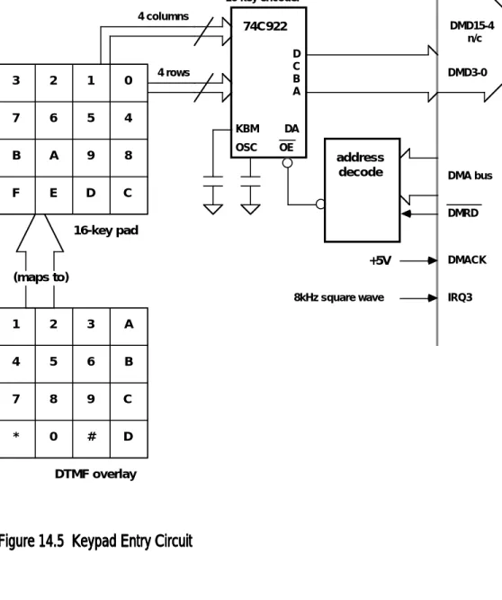
For DTMF digit entry using the keypad, a 74C922 16-key encoder chip is used in conjunction with a 16-key SPST switch matrix and address decoding circuitry. An example of this circuit is shown in Figure 14.5.
3 2 1 0
7 6 5 4
8 9 A B
C D E F
1 2 3 A
4 5 6 B
7 8 9 C
* 0 # D
16-key pad
DTMF overlay
74C922 16-key encoder
D C B A 4 columns
4 rows
KBM OSC
DA
OE address
decode DMA bus
DMRD
DMACK +5V
DMD3-0 DMD15-4
n/c
(maps to)
ADSP-2100
IRQ3 8kHz square wave
Figure 14.5 Keypad Entry Circuit Figure 14.5 Keypad Entry Circuit Figure 14.5 Keypad Entry Circuit Figure 14.5 Keypad Entry Circuit Figure 14.5 Keypad Entry Circuit
14 14 14 14 14 Dual-Tone Multi-Frequency
Dual-Tone Multi-Frequency Dual-Tone Multi-Frequency Dual-Tone Multi-Frequency Dual-Tone Multi-Frequency
451 451 451 451 451
The CMOS key encoder provides all the necessary logic to fully encode an array of SPST switches. The keyboard scan is implemented by an external capacitor. An internal debounce circuit also needs a external capacitor as shown in Figure 14.5. The Data Available (DA) output goes high when a valid keyboard entry has been made. The Data Available output returns low when the entered key is released, even if another key is pressed. The Data Available will return high to indicate acceptance of the new key after a normal debounce period. To interrupt the ADSP-2100 when a key has been pressed, invert the Data Available signal and tie it directly to one of the four independent hardware interrupt pins. An internal register in the keypad encoder chip remembers the last key pressed even after the key is released.
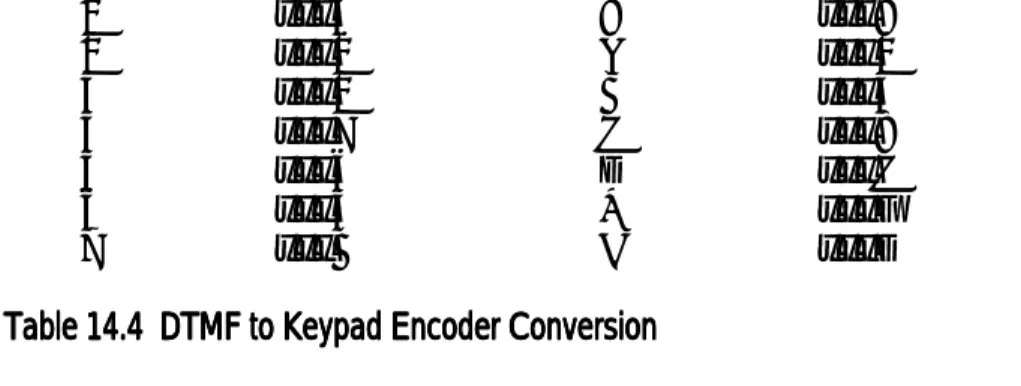
Because a DTMF keypad maps to a hexadecimal keypad as shown in Figure 14.5 and Table 14.4, a program using the keypad for digit entry would use a row and column tone look-up list which is similar to that used in Listing 14.1, but its contents would be slightly different. The operation of the tone look-up list is the same as in Listing 14.1, although the values stored in data memory within the look-up list reflect the remapping of the keypad.
DTMF Key 74C922 Output DTMF Key 74C922 Output
0 xxxE 8 xxxA
1 xxx3 9 xxx9
2 xxx2 A xxx0
3 xxx1 B xxx4
4 xxx7 C xxx8
5 xxx6 D xxxC
6 xxx5 * xxxF
7 xxxB # xxxD
Table 14.4 DTMF to Keypad Encoder Conversion Table 14.4 DTMF to Keypad Encoder Conversion Table 14.4 DTMF to Keypad Encoder Conversion Table 14.4 DTMF to Keypad Encoder Conversion Table 14.4 DTMF to Keypad Encoder Conversion
14.4.1.2 14.4.1.2 14.4.1.2 14.4.1.2
14.4.1.2 Data Memory List Data Memory List Data Memory List Data Memory List Data Memory List
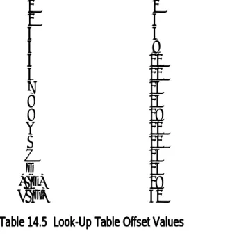
For DTMF digit entry by reading the digit in data memory (as in Listing 14.1), a row and column tone look-up list is implemented. The DTMF digits are stored in the four LSBs of the 16-bit data word. All DTMF digits are mapped to their hexadecimal numerical equivalent. The * digit is assigned to the hexadecimal number H#E, and the # digit is assigned to the hexadecimal number H#F. Table 14.5 on the next page shows this mapping. The DTMF digits are stored in such a way that you can see the DTMF sequence being dialed directly out of data memory using the ADSP-2100 Simulator or Emulator in the hexadecimal data memory display mode.
14 14 14 14 14
452 452 452 452 452
Dual-Tone Multi-Frequency Dual-Tone Multi-Frequency Dual-Tone Multi-Frequency Dual-Tone Multi-Frequency Dual-Tone Multi-Frequency
When a DTMF digit is read from data memory, the twelve upper MSBs are first masked out. Then the numerical value of the DTMF digit (0, 1,..., 15 decimal) is multiplied by 2 (yielding 0, 2,..., 30 decimal) because each entry within the look-up table is two 16-bit words long. One word holds the row frequency, and the other word holds the column frequency. This offset value is then added to the base address of the beginning of the look- up table. The resultant address is used to read the row frequency and postincremented by one. The incremented address is used to read the column frequency.
DTMF Digit Base Address Offset Value
0 0
1 2
2 4
3 6
4 8
5 10
6 12
7 14
8 16
9 18
A 20
B 22
C 24
D 26
* (E) 28
# (F) 30
Table 14.5 Look-Up Table Offset Values Table 14.5 Look-Up Table Offset Values Table 14.5 Look-Up Table Offset Values Table 14.5 Look-Up Table Offset Values Table 14.5 Look-Up Table Offset Values
For example, referring to Listing 14.1 at the label nextdigit and Figure 14.4, the DTMF digit is read out of data memory and stored in register AX0 by the instruction AX0=DM(I0,M0). For this example, assume the value in AX0 is H#0004. Control flow is passed to the instruction labeled newdigit.
The twelve MSBs are set to zero, and the result is multiplied by 2 in the barrel shifter yielding H#0008. AY0 is set to the base address (^digits) of the tone look-up table. The base address is added to the offset and placed in the I1 register. I1 now holds the value ^digits+8, M0 was previously set to 1, and L1 to 0. The instruction AX0=DM(I1,M0) reads the row
frequency (770Hz) from the look-up table and stores it in the variable hertz1 used by the sinewave generation code. I1 is automatically
postmodified by M0 (1), and the next instruction AX0=DM(I1,M0) reads the column frequency (1209Hz) and stores that in the variable hertz2 used
14 14 14 14 14 Dual-Tone Multi-Frequency
Dual-Tone Multi-Frequency Dual-Tone Multi-Frequency Dual-Tone Multi-Frequency Dual-Tone Multi-Frequency
453 453 453 453 453
by the sinewave generation code. When the sinewave generation code is executed (at the label maketones), a signal of 770Hz + 1209Hz (DTMF digit 4) is generated.
14.4.2 14.4.2 14.4.2 14.4.2
14.4.2 Dialing Demonstration Dialing Demonstration Dialing Demonstration Dialing Demonstration Dialing Demonstration
The program listed in Listing 14.1 is a DTMF dialing demonstration program. DTMF digits are read sequentially out of a linear buffer. The variable sign_dura_ms (signal duration in milliseconds) sets the length of time that a DTMF digit is generated. The variable interdigit_ms (interdigit time in milliseconds) sets the length of the silent period following a DTMF digit. When a new digit is started, the variable time_on is set to 8 x
sign_dura_ms and the variable time_off is set to 8 x interdigit_ms. Time_on and time_off are counters which the program decrements during interrupts to count the passing of time. Because the ADSP-2100 is interrupted at an 8kHz rate, the amount of time between interrupts is 1/8 millisecond (125µs). By taking the time in milliseconds and multiplying that numerical value by 8, the number of interrupts to count results.
The DTMF digit dialing list stored in data memory starting at location
^dial_list can contain values other than DTMF digits. It can also contain control words. Refer to the comment immediately following the variable declarations at the top of the source code in Listing 14.1. If a value is encountered in the dialing list which has any bits set in the four MSBs, the dialing stops. This value is used as a delimiter to terminate the dialing list.
If a value is encountered in which the four bits 15-12 are zeros, but any of the bits 11-8 are set, the dialing restarts at the top of the dialing list. If a value is encountered in which all eight bits 15-8 are zeros, but any of the bits 7-4 are set, then a quiet space of length sign_dura_ms plus interdigit_ms is generated. Finally, if all twelve bits 15-4 are zeros, then the four LSBs represent a valid DTMF digit to generate.
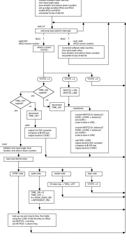
A software state machine has been implemented in the program of Listing 14.1. It is partly controlled by IRQ2, which in this example is wired to a debounced switch. The state machine has three states. Pushing the IRQ2 pushbutton moves the state machine into the next state. The current state of the machine is stored in data memory variable state. Figure 14.6, on the next page, shows the demonstration program’s state machine. The
program starts in state 0. In this state, no digits are generated. Pushing the IRQ2 pushbutton moves the machine into state 1, in which a continuous dial tone (350Hz + 400Hz) is generated. The state machine moves to state 2 when the IRQ2 pushbutton is pushed again. In state 2, the DTMF dialing list is sequentially read and DTMF digits generated. The state machine stays in state 2 until IRQ2 is pushed again or a “stop” control word is read out of the dialing list, in which case the machine jumps back to state 0.
14 14 14 14 14
454 454 454 454 454
Dual-Tone Multi-Frequency Dual-Tone Multi-Frequency Dual-Tone Multi-Frequency Dual-Tone Multi-Frequency Dual-Tone Multi-Frequency
Figure 14.6 Dialing Demonstration Program State Machine Figure 14.6 Dialing Demonstration Program State Machine Figure 14.6 Dialing Demonstration Program State Machine Figure 14.6 Dialing Demonstration Program State Machine Figure 14.6 Dialing Demonstration Program State Machine
A flowchart of the operation of this demonstration program is shown in Figure 14.7. The data memory variables row0, ..., row3, col0, ..., col3 in Listing 14.1 are initialized with their appropriate frequencies. These variables are not used by the program at all, but are included as a handy reference so you can look up the frequencies using the data memory display of the ADSP-2100 Simulator or Emulator without having to refer back to any literature.
STATE 1
STATE 2 STATE 0 start
output: silence
push IRQ2 button
output: continuous dial tone
output: DTMF tones in DM list
push IRQ2 button push IRQ2 button
"stop" control word in list or
anything but a
"stop" control word in list
14 14 14 14 14 Dual-Tone Multi-Frequency
Dual-Tone Multi-Frequency Dual-Tone Multi-Frequency Dual-Tone Multi-Frequency Dual-Tone Multi-Frequency
455 455 455 455 455
Figure 14.7 Tone Generation Block Diagram Figure 14.7 Tone Generation Block Diagram Figure 14.7 Tone Generation Block Diagram Figure 14.7 Tone Generation Block Diagram Figure 14.7 Tone Generation Block Diagram
eight kHz (IRQ3 service routine)
what is current STATE?
STATE = 0 STATE = 1
HERTZ1 = 350 HERTZ2 = 400 TIME_ON
expired?
decrement TIME_ON TIME_OFF
expired?
decrement TIME_OFF
yes no
no yes
quiet
output 0 to D/A converter compress to µ-255 law output result to CODEC
maketones
convert HERTZ1 to 'advance1' SUM1 = SUM1 + 'advance1' sin( SUM1 ) scale & store in SIN1 convert HERTZ2 to 'advance2' SUM2 = SUM2 + 'advance2' sin( SUM2 ) scale & store in SIN2 add SIN1 + SIN2 output result to D/A converter compress to µ-255 law output result to CODEC reset
initialize sine input angle, tone duration and silence down-counters
read next dial list entry
stop code restart code
quiet code DTMF code
STATE = 0 I0 index reg. = ^DIAL_LIST
TIME_ON = 0 TIME_OFF = 8 x (SIGN_DURA_MS + INTERDIGIT_MS)
look-up row and column freq. from table using four LSBs of dial list entry as offset set HERTZ1 = row freq.
set HETRZ2 = column freq.
start
initialize software state machine, sine input angle value,
tone duration and silence down-counters set up edge-sensitive IRQ2 and IRQ3 enable IRQ2 and IRQ3 set pointer to top of dial list setup
self-jump loop (wait for interrupt) wait_int
next_state (IRQ2 service routine) IRQ2
IRQ3
increment software state machine, sine input angle value,
tone duration and silence down-counters set pointer to top of dial list
STATE = 2
14 14 14 14 14
456 456 456 456 456
Dual-Tone Multi-Frequency Dual-Tone Multi-Frequency Dual-Tone Multi-Frequency Dual-Tone Multi-Frequency Dual-Tone Multi-Frequency
14.4.3 14.4.3 14.4.3 14.4.3
14.4.3 Multi-Channel Generation Multi-Channel Generation Multi-Channel Generation Multi-Channel Generation Multi-Channel Generation
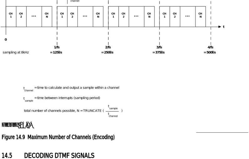
A single ADSP-2100 can generate simultaneous DTMF signals for many channels in real time. The multi-channel program uses the same method as the single channel version, but each channel has its own scratchpad variables and memory-mapped I/O ports. The channels are computed sequentially in time every time an interrupt occurs. See Figure 14.8 and
CH 5 CH 4 CH 3 CH 2 CH 1 Data Memory
RAM
CODEC
en CH 6
data in analog out
CODEC
en CH 5
data in analog out
CODEC
en CH 4
data in analog out
CODEC
en CH 3
data in analog out
CODEC
en CH 2 data in
analog out CODEC
en CH 1 data in
analog out
CH 6
en abcd
o o o o o o o o o o o o
enables
address decoder
wait state generator
PAL DMA
DMA
DMWR DMWR DMRD
DMRD o
o
DMD
DMA
DMRD DMWR DMACK
PMD
PMA
PMRD PMS
Program Memory
OE CS Data
Adr
IRQ3
8 kHz
CS Data Adr OE WE
ADSP- 2100
•
•
•
•
•
•
WAIT KEYPAD CH 6
Figure 14.8 Six-Channel Schematic Figure 14.8 Six-Channel Schematic Figure 14.8 Six-Channel Schematic Figure 14.8 Six-Channel Schematic Figure 14.8 Six-Channel Schematic
keypad
14 14 14 14 14 Dual-Tone Multi-Frequency
Dual-Tone Multi-Frequency Dual-Tone Multi-Frequency Dual-Tone Multi-Frequency Dual-Tone Multi-Frequency
457 457 457 457 457
CH 1
CH 2
CH
• • • N
CH 1
CH 2
CH
• • • N
CH 1
CH 2
CH
• • • N CH
1 CH
2
CH
• • • N
0
t tsample
tchannel
1/fs 2/fs 3/fs 4/fs
= 500µs
= 375µs
= 250µs
= 125µs sampling at 8kHz
tsample
tchannel= time to calculate and output a sample within a channel
= time between interrupts (sampling period)
total number of channels possible, N = TRUNCATE ( tsample
tchannel )
Figure 14.9.
Figure 14.9 Maximum Number of Channels (Encoding) Figure 14.9 Maximum Number of Channels (Encoding) Figure 14.9 Maximum Number of Channels (Encoding) Figure 14.9 Maximum Number of Channels (Encoding) Figure 14.9 Maximum Number of Channels (Encoding)
14.5 14.5 14.5 14.5
14.5 DECODING DTMF SIGNALS DECODING DTMF SIGNALS DECODING DTMF SIGNALS DECODING DTMF SIGNALS DECODING DTMF SIGNALS
Decoding a DTMF signal involves extracting the two tones in the signal and determining from their values the intended DTMF digit. Tone
detection is often done in analog circuits by detecting and counting zero- crossings of the input signal. In digital circuits, tone detection is easier to accomplish by mathematically transforming the input time-domain signal into its frequency-domain equivalent by means of the Fourier transform.
14.5.1 14.5.1 14.5.1 14.5.1
14.5.1 DFTs and FFTs DFTs and FFTs DFTs and FFTs DFTs and FFTs DFTs and FFTs
The discrete Fourier transform (DFT) or fast Fourier transform (FFT) can be used to transform discrete time-domain signals into their discrete frequency-domain components. The FFT (described in Chapter 7, Fast Fourier Transforms) efficiently calculates all possible frequency points in the DFT (e.g., a 256-point FFT computes all 256 frequency points). On the other hand, the DFT can be computed directly to yield only some of the
14 14 14 14 14
458 458 458 458 458
Dual-Tone Multi-Frequency Dual-Tone Multi-Frequency Dual-Tone Multi-Frequency Dual-Tone Multi-Frequency Dual-Tone Multi-Frequency
points, for example, only the 20th, 25th, and 30th frequency points out of the possible 256 frequency points. Typically, if more than log2N of N points are desired, it is quicker to compute all the N points using an FFT and discard the unwanted points. If only a few points are needed, the DFT is faster to compute than the FFT. The DFT is faster for finding only eight tones in the full telephone-channel bandwidth.
The definition of an N-point DFT is as follows:
A single frequency point of the N points is found by computing the DFT
for only one k index within the range 0 ≤ k ≤ N–1. For example, if k=15:
14.5.2 14.5.2 14.5.2 14.5.2
14.5.2 Goertzel Algorithm Goertzel Algorithm Goertzel Algorithm Goertzel Algorithm Goertzel Algorithm
The Goertzel algorithm evaluates the DFT with a savings of computation and time. To compute a DFT directly, many complex coefficients are required. For an N-point DFT, N2 complex coefficients are needed. Even for just a single frequency in a N-point DFT, the DFT must calculate (or look up) N complex coefficients. The Goertzel algorithm needs only two coefficients for every frequency: one real coefficient and one complex coefficient.
The Goertzel algorithm computes a complex, frequency-domain result just as a DFT does, but the Goertzel algorithm can be modified algebraically so that the result is the square of the magnitude of the frequency component (a real value). This modification removes the phase information, which is irrelevant in the tone detection application. The advantage of this
modification is that it allows the algorithm to detect a tone using only one, real coefficient.
Not only is the number of coefficients reduced, but the Goertzel algorithm can process each sample as it arrives. There is no need to buffer N samples before computing the N-point DFT, nor do any bit-reversing or
windowing. As shown in Figure 14.10, the Goertzel algorithm can be though of as a second-order IIR filter.
X(15) =
∑
n=0 N–1
x(n)WN15n where k = 15 and WN15n= e–j(2π/N)15n
X(k) =
∑
n=0 N–1
x(n)WNnk where k = 0, 1, ... , N–1 and WNnk = e–j(2π/N)nk
14 14 14 14 14 Dual-Tone Multi-Frequency
Dual-Tone Multi-Frequency Dual-Tone Multi-Frequency Dual-Tone Multi-Frequency Dual-Tone Multi-Frequency
459 459 459 459 459
feedforward feedback
X(k)
= N
2π
k –W
Nk = –e z–1
coef
coef 2cos –j2πk/N
–WN k
y (N)k x(n)
–1
z–1
k
=
n = 0, 1, ..., N–1 n = N
k
Figure 14.10 Goertzel Algorithm Figure 14.10 Goertzel Algorithm Figure 14.10 Goertzel Algorithm Figure 14.10 Goertzel Algorithm Figure 14.10 Goertzel Algorithm
The Goertzel algorithm can be used to compute a DFT; however, its implementation has much in common with filters. A DFT or FFT
computes a buffer of N output data items from a buffer of N input data items. The transform is accomplished by first filling an input buffer with data, then computing the transform of those N samples, yielding N
results. By contrast, an IIR or FIR filter computes a new output result with each occurrence of a new input sample. The second-order recursive
computation of the DFT by means of the Goertzel algorithm as shown in Figure 14.10 computes a new yk(n) output for every new input sample x(n). The DFT result, X(k), is equivalent to yk(n) when n=N, i.e.,
X(k)=yk(N). Since any other value of yk(n), in which n≠N, does not contribute to the end result X(k), there is no need to compute yk(n) until n=N. This implies that the Goertzel algorithm is functionally equivalent to a second-order IIR filter, except that the one output result of the filter is generated only after N input samples have occurred.
Computation of the Goertzel algorithm can be divided into two phases.
The first phase involves computing the feedback legs in Figure 14.10 as depicted in Figure 14.11 on the next page. The second phase evaluates X(k) by computing the feedforward leg in Figure 14.10 as shown in Figure 14.12, also on the next page.
14 14 14 14 14
460 460 460 460 460
Dual-Tone Multi-Frequency Dual-Tone Multi-Frequency Dual-Tone Multi-Frequency Dual-Tone Multi-Frequency Dual-Tone Multi-Frequency
= N
2π k
z–1 coef
coef 2cos x(n)
–1
z–1
k
n = 0, 1, ..., N–1
k
Qn
Qn–1
Figure 14.11 Feedback Phase Figure 14.11 Feedback Phase Figure 14.11 Feedback Phase Figure 14.11 Feedback Phase Figure 14.11 Feedback Phase
X(k)
–WNk = –e –j2πk/N
y (N)k = n = N
Qn
Qn–1
QN–1
QN–2
=
=
Figure 14.12 Feedforward Phase
Figure 14.12 Feedforward Phase
Figure 14.12 Feedforward Phase
Figure 14.12 Feedforward Phase
Figure 14.12 Feedforward Phase
14 14 14 14 14 Dual-Tone Multi-Frequency
Dual-Tone Multi-Frequency Dual-Tone Multi-Frequency Dual-Tone Multi-Frequency Dual-Tone Multi-Frequency
461 461 461 461 461
yk(N) = Qk(N–1) – WNk Qk(N–2) = X(k)
14.5.2.1 14.5.2.1 14.5.2.1 14.5.2.1
14.5.2.1 Feedback Phase Feedback Phase Feedback Phase Feedback Phase Feedback Phase
The feedback phase occurs for N input samples (counted as n=0, 1,..., N–
1). During this phase, two intermediate values Q(n) and Q(n–1) are stored in data memory. Their values are evaluated as follows:
Qk(n) = coefk x Qk(n–1) – Qk(n–2) + x(n) where:
coefk = 2 cos(2πk/N) Qk(–1) = 0
Qk(–2) = 0
n = 0, 1, 2, ..., N–1
Qk(n–1) and Qk(n–2) are the two feedback storage elements for frequency point k and x(n) is the current input sample value Upon each new sample x(n), Q(n–1) and Q(n–2) are read out of data memory and used to evaluate a new Q(n). This new Q(n) is stored where the old Q(n) was. That old Q(n) value is put where the old Q(n–1) was.
This action updates Q(n–1) and Q(n–2) for every sample.
14.5.2.2 14.5.2.2 14.5.2.2 14.5.2.2
14.5.2.2 Feedforward Phase Feedforward Phase Feedforward Phase Feedforward Phase Feedforward Phase
The feedforward phase occurs once after the feedback phase has been performed for N input samples. The feedforward phase generates an output sample. During computation of the feedforward phase, no new input is used, i.e., new inputs are ignored. As shown in Figure 14.12, the complex value X(k), equivalent to the same X(k) calculated by a DFT, is computed using the two intermediate values Q(n) and Q(n–1) from the feedback phase calculations. At this time, those two intermediate values
are Q(N–1) and Q(N–2) since n=N–1. X(k) is calculated as follows:
As stated previously, tone detection does not require phase information, and through some algebraic manipulation, the Goertzel algorithm can be modified to output only the squares of the magnitudes of X(k)
(magnitudes squared). This implementation not only saves time needed to compute the magnitude squared from a complex result, but also
eliminates the need to do any complex arithmetic. The modified Goertzel algorithm is exactly the same as the Goertzel algorithm during the
14 14 14 14 14
462 462 462 462 462
Dual-Tone Multi-Frequency Dual-Tone Multi-Frequency Dual-Tone Multi-Frequency Dual-Tone Multi-Frequency Dual-Tone Multi-Frequency
feedback phase, but the feedforward phase is simplified. The magnitude squared of the complex result is expanded in terms of the values available at the end of the feedback iterations. The complex coefficient thereby becomes unnecessary, and the only coefficient needed is conveniently the same as the real coefficient previously used in the feedback phase. The
formula for the magnitude squared is derived as follows:
yk(N) 2 = X(k)
2
yk(N) 2 = A2 + B2 - AB coefk where coef k = 2 cos N2π k
= A2 - AB (2cos ø) + B2
= A2 - 2AB cos ø + B2(cos2ø + sin2ø )
= A2 - 2AB cos ø + B2cos2ø + B2sin2ø
= (A - B cos ø)2 + (B sin ø)2 yk(N) 2 = (Real Part)2 + (Imag. Part)2
= A - B cos ø + j B sin ø
= A - B [ cos ø - j sin ø ]
= A - B-j ø
= A - B e
-j N 2πk
= A - B WNk
yk(N) = Qk(N-1) - WNk Qk(N-2)
14 14 14 14 14 Dual-Tone Multi-Frequency
Dual-Tone Multi-Frequency Dual-Tone Multi-Frequency Dual-Tone Multi-Frequency Dual-Tone Multi-Frequency
463 463 463 463 463
The DTMF decoder calculates magnitudes squared of all eight fundamental tones as well as the magnitude squared of each
fundamental’s second harmonic. This information is used in one of the validation tests to determine if tones received make up a valid DTMF digit. Specifically, it will be used to give the DTMF decoder the ability to discriminate between pure DTMF sinusoids and speech. Speech
waveforms may also contain sinusoids similar to DTMF digits, but speech also has energy in higher-order harmonics, typically the second harmonic.
This test is described later.
The modified Goertzel algorithms (one for each k value) have the ability to detect tones using less computation time and fewer stored coefficients than an equivalent DFT would require. For each frequency to detect, the modified Goertzel algorithms need only one real coefficient. This
coefficient is used both in the feedback and feedforward phases.
14.5.2.3 14.5.2.3 14.5.2.3 14.5.2.3
14.5.2.3 Choosing N and k Choosing N and k Choosing N and k Choosing N and k Choosing N and k
Determining the coefficient’s value for a given tone frequency involves a trade off between accuracy and detection time. These parameters are dependent on the value chosen for N. If N is very large, resolution in the frequency domain is very good, but the length of time between output samples increases, because the feedback phase of Goertzel algorithm is executed N times (once on each input sample) before the feedforward phase is executed once (yielding a single output sample).
If tone detection had been implemented using FFTs, the values of N would have been limited to those that were a power of the radix of the FFT: 16 point, 32 point, 64 point, 128 point, 256 point, etc. for radix-2 (power of 2) FFTs and 16 point, 64 point, 256 point, 1024 point, etc. for radix-4 (power of 4) FFTs. DFTs and Goertzel algorithms, however, are not limited to any radix. These can be computed using any integer value for N.
When an N-point DFT is being evaluated, N input samples (equally spaced in time) are processed to yield N output samples (equally spaced in frequency). The N output samples are:
X(k) where k = 0, 1, 2, ... , N–1
The spacing of the output samples is determined by half the sampling frequency divided by N. If some tone is present in the input signal which does not fall exactly on one of these points in the frequency domain, its
14 14 14 14 14
464 464 464 464 464
Dual-Tone Multi-Frequency Dual-Tone Multi-Frequency Dual-Tone Multi-Frequency Dual-Tone Multi-Frequency Dual-Tone Multi-Frequency
frequency component appears partly in the closest frequency point, and partly in the other frequency points. This phenomenon is called leakage.
To avoid leakage, it is desirable for all the tones to be detected to be exactly centered on a frequency point. The discrete frequency points are referenced by their k value. The value of k can be any integer within the range 0, 1, 2, ..., N–1. The actual frequency to which k corresponds is dependent on the sampling frequency and N as determined by the
ftone fsampling
k
= N following formula:
or
k = N
fsampling •ftone
where ftone is the tone frequency being detected and k is an integer.
Since the sampling frequency is set at 8kHz by the telephone system, and the tones to detect are the DTMF tones, which are also set, the only
variable we can modify is N. The numbers k must be integers, so the corresponding frequency points may not be exactly the DTMF frequencies desired. The corresponding absolute error is defined as the difference between what k would be if it could be any real number and the closest
integer to that optimal value. For example:
Bell Labs specifically chose the DTMF tones such that they would not be harmonically related. This makes it difficult to choose a value N for which all tones exactly match the DTMF frequency points. A solution could be to perform separate Goertzel algorithms (each with a different value of N) for each tone, but that would involve a lot of non-computational processor overhead. Instead, in this example, values of N were chosen for which the maximum absolute k error of any one of the tones was considered
acceptably small. Then, the length of time to detect a tone (which is absolute k error = Nftone
fsampling – CLOSEST INTEGER
Nftone fsampling
14 14 14 14 14 Dual-Tone Multi-Frequency
Dual-Tone Multi-Frequency Dual-Tone Multi-Frequency Dual-Tone Multi-Frequency Dual-Tone Multi-Frequency
465 465 465 465 465
proportional to the sampling rate multiplied by N) was taken into consideration. The value of N best suited for detecting the eight DTMF fundamental tone frequencies was chosen to be 205. The value of N best suited for detecting the eight second harmonic frequencies was chosen to be 201. See Table 14.6 for the corresponding k values and their respective absolute errors. These values of k allow Goertzel outputs to occur
approximately once every 26 milliseconds.
Fundamental k value k value Absolute coefk
Frequency floating-point nearest integer k error (N=205)
697.0Hz 17.861 18 0.139 1.703275
770.0Hz 19.731 20 0.269 1.635859
852.0Hz 21.833 22 0.167 1.562297
941.0Hz 24.113 24 0.113 1.482867
1209.0Hz 30.981 31 0.019 1.163138
1336.0Hz 34.235 34 0.235 1.008835
1477.0Hz 37.848 38 0.152 0.790074
1633.0Hz 41.846 42 0.154 0.559454
Second Harmonic (N=201)
1394.0Hz 35.024 35 0.024 0.917716
1540.0Hz 38.692 39 0.308 0.688934
1704.0Hz 42.813 43 0.187 0.449394
1882.0Hz 47.285 47 0.285 0.202838
2418.0Hz 60.752 61 0.248 –0.659504
2672.0Hz 67.134 67 0.134 –1.000000
2954.0Hz 74.219 74 0.219 –1.352140
3266.0Hz 82.058 82 0.058 –1.674783
sampling frequency = 8kHz
Table 14.6 Values of k and Absolute k Error Table 14.6 Values of k and Absolute k Error Table 14.6 Values of k and Absolute k Error Table 14.6 Values of k and Absolute k Error Table 14.6 Values of k and Absolute k Error
14.5.3 14.5.3 14.5.3 14.5.3
14.5.3 DTMF Decoding Program DTMF Decoding Program DTMF Decoding Program DTMF Decoding Program DTMF Decoding Program
For DTMF decoding, the ADSP-2100 solves sixteen separate modified Goertzel algorithms, eight of length 205 to detect the DTMF fundamentals, and eight of length 201 to detect the DTMF second harmonics. To
14 14 14 14 14
466 466 466 466 466
Dual-Tone Multi-Frequency Dual-Tone Multi-Frequency Dual-Tone Multi-Frequency Dual-Tone Multi-Frequency Dual-Tone Multi-Frequency
implement concurrent Goertzel algorithms of lengths 205 and 201, the feedback phase iterations of all the Goertzel algorithms (fundamentals and second harmonics) are performed for 201 samples (n=0, 1,..., 200). For the next four samples, only the Goertzel algorithms of length 205
(fundamentals) are iterated (n=201, 202, 203, 204). The other Goertzel algorithms of length 201 (second harmonics) ignore the new samples. On the last iteration, when n=N=205, all the feedforward phases are evaluated (both fundamentals and second harmonics), and any new input samples at that time are ignored. In the DTMF decoder application presented here which uses the modified Goertzel algorithm, the magnitude squared calculations are performed for the feedforward phases.
DTMF decoding is done in two major tasks, as shown in the block
diagram in Figure 14.13. The first task solves sixteen Goertzel algorithms to calculate the magnitudes squared of tone frequencies present in the input signal, then the second task tests the frequency results to determine if the tones detected constitute a valid DTMF digit. The first task spans N+1 processor interrupts, N for the feedback phases of the Goertzel algorithms, then one more for the feedforward phases. The second task immediately follows completion of all sixteen feedforward phases. The length of time required by the processor for this testing may span the next few interrupts (during which time new input samples are ignored), but since the number of input samples lost is small compared to the number of interrupts serviced during the Goertzel evaluations, the loss is
insignificant (see Figure 14.15). The Goertzel algorithms are not sensitive to incoming signal phase, and therefore no phase synchronization is attempted.
14.5.3.1 14.5.3.1 14.5.3.1 14.5.3.1
14.5.3.1 Input Scaling Input Scaling Input Scaling Input Scaling Input Scaling
It is important to notice that the input sample values are scaled down by eight bits to eliminate the possibility of overflows within 205 iterations of the feedback phase. Scaling by eight bits increases the quantization error of the input samples, but this does not affect the effectiveness of the
decoder. Input samples are read from a µ-law-compressed codec. The 8-bit data values are used as offset values to a µ-law-to-linear conversion look- up table. The corresponding linear values are scaled such that the input samples range from H#007F to H#FF80 instead of the normalized equivalent range of H#7FFF to H#8000.
14 14 14 14 14 Dual-Tone Multi-Frequency
Dual-Tone Multi-Frequency Dual-Tone Multi-Frequency Dual-Tone Multi-Frequency Dual-Tone Multi-Frequency
467 467 467 467 467
wait for interrupt
read sample
from CODEC linear expansion
Goertzel calculations
2x697 Hz (N=201)
Goertzel 2x770
Hz
Goertzel 2x852
Hz
Goertzel 2x941
Hz
Goertzel 2x1209 Hz
Goertzel 2x1336
Hz
Goertzel 2x1477
Hz
Goertzel 2x1633
Hz Goertzel
calculations for 697 Hz (N=205)
Goertzel 770 Hz
Goertzel 852 Hz
Goertzel 941 Hz
Goertzel 1209 Hz
Goertzel 1336 Hz
Goertzel 1477 Hz
Goertzel 1633 Hz
is the twist acceptable?
are the associated second harmonics below their acceptable threshold values?
set 'outputcode' to invalid
set 'outputcode' to value specified
by DTMF map
is 'outputcode' new since last decode operation?
send 'outputcode' fail
fail
fail
chose the row which is above the minimum tone-present threshold and make sure no other rows are above the
maximum tone-not-present threshold
row and col tests pass
chose the column which is above the minimum tone-present threshold and make sure no other columns are above the
maximum tone-not-present threshold
fail row and
col tests pass
pass
no
yes IRQ
received
only up to here if n=201, 202,203,204
continue only if n=205,
otherwise return
return
return
choose one choose one
pass
14 14 14 14 14
468 468 468 468 468
Dual-Tone Multi-Frequency Dual-Tone Multi-Frequency Dual-Tone Multi-Frequency Dual-Tone Multi-Frequency Dual-Tone Multi-Frequency
Figure 14.13 Tone Decoder Block Diagram Figure 14.13 Tone Decoder Block Diagram Figure 14.13 Tone Decoder Block Diagram Figure 14.13 Tone Decoder Block Diagram Figure 14.13 Tone Decoder Block Diagram
14.5.3.2 14.5.3.2 14.5.3.2 14.5.3.2
14.5.3.2 Multi-Channel DTMF Decoder Software Multi-Channel DTMF Decoder Software Multi-Channel DTMF Decoder Software Multi-Channel DTMF Decoder Software Multi-Channel DTMF Decoder Software
An example of a multi-channel DTMF decoder is given in Listing 14.2.
This example is a 6-channel version, although at least twelve channels can be decoded by an ADSP-2100A running at a 12.5MHz instruction rate. The six channels are labeled channel A, channel B, ..., channel F. The following software description gives an overview of the variables and constants used, then outlines the core executive routine and describes the interrupt service routine. The macros and subroutines are explained as needed.
14.5.3.3 14.5.3.3 14.5.3.3 14.5.3.3
14.5.3.3 Constants, Variables and I/O Ports Constants, Variables and I/O Ports Constants, Variables and I/O Ports Constants, Variables and I/O Ports Constants, Variables and I/O Ports
The number of channels to decode is specified in the .CONST declaration section. The number of channels must be greater than one and less than or equal to the maximum number of channels allowed, which is dependent on the processor cycle time. The faster the processor cycle time, the more channels can be decoded in real time. The limiting factor is how many of the Goertzel feedback operations can be performed between successive processor interrupts (see Figure 14.14). To decode a single channel only, the source code must be slightly altered. The only necessary alteration involves the circular buffer of length channels which stores the input samples; this buffer must be changed to a single data memory variable.
Although not necessary, other alterations can be done to optimize the software for a single channel if desired.
The hexadecimal value which the decoder outputs when no DTMF digit is received is defined by the constant called baddigitcode. For debugging purposes, a variable called failurecode was incorporated into each channel.
This variable is assigned a value whether or not a valid DTMF digit was received. If a valid digit was received, failurecode is set to zero. A nonzero failurecode means that the signals received failed one of the qualifying tests. The failurecode value, defined in the constant declaration section, identifies which test failed.
The data variables are separated into two functional groups:
housekeeping variables and individual-channel variables. The
housekeeping variables are used by the software shared by all sections of the decoder. The individual channel variables are used to keep track of specifics for each channel separately. The variables are explained in detail in Listing 14.2.
The input port for each channel is a codec. The output port for each
14 14 14 14 14 Dual-Tone Multi-Frequency
Dual-Tone Multi-Frequency Dual-Tone Multi-Frequency Dual-Tone Multi-Frequency Dual-Tone Multi-Frequency
469 469 469 469 469
channel is a D/A converter in this example. In a more realistic application, such as a PBX, switching machine, or electronic voice-mail system, the output would probably be sent to dual-port memory or a mailbox register for use by another processor.
The initialization directives set up some of the static, housekeeping variables. The Goertzel coefficients are initialized as well as the µ-law-to- linear look-up table, thresholds for the received signal levels and twist test limits. (The file containing the µ-law look-up values is not included in the program listings; however, it is included in the diskette that contains the programs in this manual, which is available from your local Analog Devices Sales Office.) These initializations could be adjusted for
application-specific requirements, such as meeting the specifications of other administrations or operating as a DTMF signal tester.
To decode more or fewer than six channels, simply add or remove sections identified by the comment “edit this for more channels” in the source code listing.
14.5.3.4 14.5.3.4 14.5.3.4 14.5.3.4
14.5.3.4 Main Code Main Code Main Code Main Code Main Code
The main code section is very simple. The processor is initialized for the decoding operation, then put into an endless loop, waiting for interrupts that occur at the sampling rate (8kHz). After the ADSP-2100 is reset, the first task is to set up the static environment, such as the M and L registers in both data address generators and the ICNTL register. This task is done only once since these initializations are never changed. This set-up is performed by the subroutine called setup. Another subroutine called restart then initializes other variables which are needed for the decoding operation, but which change and must therefore be reinitialized after each decode operation. The specific tasks here include resetting the I registers of the data address generators to the top of their associated buffers,
zeroing out the delay elements for the Goertzel algorithm implementation (Q values), and resetting the counters which keep track of the input
sample number (n). The restart routine is called after every decode operation, immediately after completion of the digit validation tests, as well as before the very first decode operation.
14.5.3.5 14.5.3.5 14.5.3.5 14.5.3.5