This article shows that an additional and perhaps alternative explanation for the dollarization hysteresis is the existence of network externalities in currency demand. 1999: 1), dollarization could be defined as "residents holding a significant proportion of their wealth in the form of assets denominated in foreign currency".

Ratchet E¤ects
There are several different explanations for the dollarization hysteresis, which can generally be seen as different explanations for the existence of "ratchet effects" in the demand for money. In addition, we focus on a third explanation for the presence of knock-on effects, which is described below: the existence of network externalities in the use of currency.
Network Externalities
Now consider the reverse case, where the buyer holds dollars, while the seller prefers to hold rubles in the next period (i.e., the lower left cell of the matrix). As mentioned earlier, this is risky in the sense that the amount of the transaction is confiscated with probability q.

Best Response Functions
To ensure that the resulting values for pi;t are between 0 and 1, and to make the model econometrically estimable, a standard assumption in discrete choice theory is to assume that ²¤i;t and²i;t are i.i.d. First, it says that the probability that a given buyer will hold dollars depends on pbt+1; increases with expected depreciation, just as predicted by standard portfolio balance models.21. The fact that logistic distribution is commonly used for discrete choice models is obviously not sufficient to justify its use.
Note that, as for example in Calvo and Vegh (1995), we could have assumed that the domestic interest rate is the opportunity cost of holding rubles, while the foreign interest rate is the opportunity cost of holding dollars. Second, the conditional probability that i holds dollars decreases with the expected risk of conscationbqt+1, which seems natural, but increases with the expected tax rateb¿t+1; which seems less intuitive. However, on closer inspection, the latter result follows from the fact that the tax is one-sided and only has to be paid by buyers who hold rubles, but are matched with sellers who prefer dollars.
Finally, the e¤ect of the expected shoe leather costs, b¾t+1, is ambiguous and depends on pbt+1.
Expectations
For bpt+1 < 0:5, i.e. relatively low (expected) dollarization rate in period t+ 1, an increase in ¾bt+1 will have a negative effect on pi;t, thereby reducing agent i's demand for dollars in the current period. Myopic expectations imply xbt+1 = xt for all variables except the expected dollarization ratio, where we get bpt+1 =pt¡1, since agents who are sellers at time t+ 1 are expected to behave in the same way as they were during the previous period when they were sellers, which is timet¡1.23. While the myopic expectations assumption seems reasonable for variables such as the cost of shoe leather, the foreign currency tax rate, and the risk of confiscation, this assumption seems less reasonable for the rate of ruble depreciation, which is somewhat predictable. based on information about the growth rate of money, the spread of returns on assets in rubles and dollars, etc.
Without attempting to explicitly model this exchange rate formation process, we will for now just assume that the expected rate of ruble depreciation is in fact the. An interesting extension of the model would therefore be to introduce a search process through which agents gradually learn the correct dollarization ratio in the economy. Although there is no closed-form solution for p¤, we can plot equation 7 on a graph, and change the values of one or more fundamentals to see how the steady-state dollarization ratio is determined.
Interestingly, as shown in the analysis below, p¤ does not necessarily increase with depreciation as portfolio balance models suggest.
Steady States and Dynamics
That is, when the dollarization ratio starts slightly below this steady state, it will decrease in the next period, and will continue to decrease until the lower steady state is reached. Conversely, when the dollarization ratio begins at a level slightly above the intermediate steady state, dollarization will rise in the subsequent period, and will continue to rise until the upper steady state is reached. Although not drawn in the phase diagram, one can similarly see that, when dollarization is temporarily below the lower steady state, it will increase again, and when dollarization is temporarily above the upper steady state, it will fall back to this steady state state.
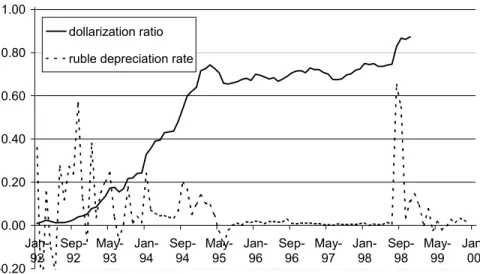
Moreover, this model shows that network externalities can explain dollarization hysteresis even in the absence of ratcheting variables. In the appendix, we compare these CMIR data with another estimate of the dollar currency in circulation that can be obtained from the Central Bank of the Russian Federation (CBR), and we conclude that the CMIR data represent the best available estimate. ² e: depreciation rate of the ruble, measured as the growth rate of the nominal ruble/dollar exchange rate at the end of the month, as published by MICEX, and included in the RET database.
Given that the vast majority of all foreign currency in Russia appears to be held in the form of U.S.
Results
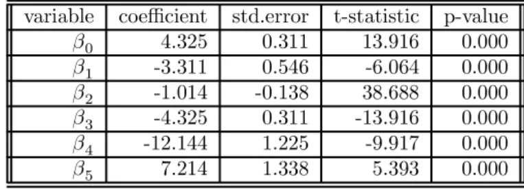
Furthermore, the p-value for the Jarque-Bera test is essentially zero, indicating that the residuals are approximately normal. However, when 24 lags are included, this test statistic is no longer significant ... at the 5 percent level. Since the null hypothesis underlying this test is that the errors are both homoscedastic and independent of the regressors and that the linear specification of the model is correct, rejection of the null means that at least one of these conditions is violated.
Assuming that the model specification is correct, then ordinary least squares parameter estimates are still robust even in the presence of heteroscedasticity and autocorrelation. Whether this is a problem, however, depends on whether one believes that the true standard errors can possibly be so large that the parameter estimates will become irrelevant ... negligible. Given that the OLS standard errors are essentially zero for almost all parameters, this seems quite unlikely.28.
2 8 For example, reestimating the model using White heteroskedasticity consistent and Newey-West heteroskedasticity and autocorrelation consistent covariance estimates still produced highly significant parameter estimates for all parameters.
Interpretation
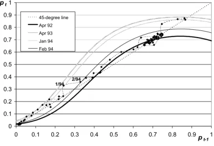
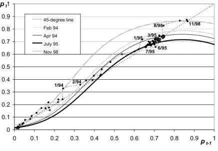
At the beginning of the 1990s, the economy started in the lower steady state with a dollarization ratio close to zero (in Soviet times, the purchase of foreign currency was severely punished). While the lower steady state is still stable in April 1992, this steady state disappeared by April 1993, causing an increase in dollarization. Then, in February 1994, both depreciation and the rate variable fall, causing the curve to shift down and the lower steady state to reappear.
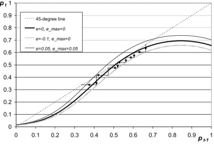
However, as shown in the chart, the "2/94" point lies above the intermediate unstable steady state of the curve, causing the dollarization ratio to move toward the upper rather than the lower steady state. As the middle curve shows, a simple stabilization of the exchange rate (e= 0) is not sufficient for a phase transition, even if the stabilization lasts long enough so that max= 0: Once the ruble starts to appreciate, however, the share the upper steady state disappears and a dynamic adjustment process is set in motion that causes the dollarization ratio to fall to the lower steady state. Note that the rate of appreciation need not be maintained until the lowest steady state is actually reached.
This would then be sufficient to allow dollarization to naturally decline further until the lower steady state is reached.
Fiscal Policy
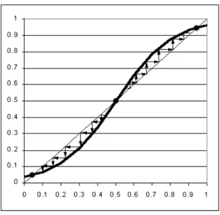
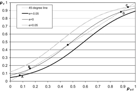
The arrows in Figure 7 show that a temporary ruble appreciation of 5 percent per month, if sustained for at least four consecutive months, is sufficient to permanently reduce dollarization. As can be seen again in Figure 7, an appreciation rate of 5 percent sustained for six consecutive months (resulting in a total appreciation of 34 percent) could be followed by a subsequent ruble depreciation of 5 percent for six months. months without dollarization returning to the above stable state. The question then is whether the removal of the tax will cause a downward shift large enough to cause a phase transition, i.e. whether it will cause the upper steady state to disappear.
Simply reducing the tax rate from ¿ = 0:01 to ¿ = 0 has an almost imperceptible effect on the position of the curve, and therefore on dollarization.34 In other words, if everything else remained the same, the model predicts that the proposed abolition of the foreign exchange tax in 2003 is unlikely to have any effect on dollarization in Russia. That is, if the tax rate is reset to zero after those four months, the dollarization ratio at that point is below the intermediate steady state of the¿ = 0 curve, so dollarization will continue to decline by itself until it reaches the lower steady state. Only in those exceptional cases could the elimination of the foreign exchange tax have a drastic effect on dollarization.
3 5 Interestingly, this essentially amounts to an appreciation of the ruble by 5%, which coincides with the policy proposed in the previous subsection.
Enforcement Policy
Ha(1995): “Measurement of Cocirculation of Currencies”, Working Paper 95/34, International Monetary Fund, reprinted in Mizen and Pentecost (1996), chapter 4. Mueller (1999): “Ratchet E¤ects in currency substitution: An Application to the Kyrgyz Republic”, Working Paper 99/102, International Monetary Fund. 1997): “Waehurngssubstitution und Waehrungswettbewerb - Eine Marktgetriebene Waehurngsreform Fuer Russland”, Ph.D. Mueller, J.(1994): “Dollarization in Lebanon”, Working Paper 94/12, International Monetary Fund. 1998): “Personal Savings”, Information Bulletin 7, Russian Bureau of Economic Analysis, Moscow.
A. (1996): “Dollarization in Latin America: Recent Evidence and Some Policy Issues”, Working Paper 96/4, International Monetary Fund. "Competition Money and the Great Polish Contagion of 1989," Working Paper 682, Department of Economics, University of California, Los Angeles. "Currency Substitution and the Regressivity of Nonnational Taxation," Working Paper 656, Department of Economics, University of California, Los Angeles.
CMIR and CBR data are, in a sense, two sides of the same coin. The main advantage of the CMIR estimate is that it includes all registered amounts that are physically transferred to or from Russia. Therefore, it is not surprising that the dollarization ratio estimated based on CBR data.