POLITICAL BUDGET CYCLES IN THE EUROPEAN UNION: NEW EVIDENCE OF FRAGMENTATION*
Milan BEDNÁŘ
(Received: 16 April 2018; revision received: 16 July 2018;
accepted: 27 October 2018)
This paper deals with the possible existence of political budget cycles (PBCs) within the European Union (EU). I use panel data for 28 EU countries from 1995 to 2016 and provide estimates based on dynamic panel regressions. I employ a system-GMM estimator complemented by the Principal Component Analysis (PCA) to limit the number of instruments. The specifi cations include struc- tural budget balances related to the potential GDP, thereby limiting the initial endogeneity. These measures capture the true motivation behind fi scal policies. The results suggest that the EU member states exhibit PBCs: (i) the intervention occurs in the year before elections and (ii) the structural budget balance to the potential GDP ratio is lower by –0.41 percentage points a year before elec- tions. In addition, I have investigated the EU fragmentation in terms of the PBCs and selected 8 countries’ characteristics correlating to the existence of these cycles. These include lower GDP per capita, post-communist background, low tax burden, high perceived corruption, low levels of media freedom and internet usage, lower number of directly voted-in legislative offi cials, and a low parliamentary voter turnout.
Keywords: political budget cycles, fi scal policy, elections, European Union, dynamic panel estimation
JEL classifi cation indices: E62, P16, C33
* The author would like to thank the two anonymous reviewers for their valuable comments.
Milan Bednář, Ph.D. student at the University of Economics, Prague, Czech Republic. E-mail:
milan.bednar@vse.cz
INTRODUCTION
Increased budget expenditures shortly before elections to maximise votes is a widely known phenomenon. To understand this, the concept of political budg- et cycles (PBCs) can help in many areas. For example, I may be interested in whether the most-indebted Southern EU countries suffer from such manipula- tions more than the other countries. Another interesting question is whether PBCs played a role in the 2007–2008 financial crisis. The purpose of this paper is to empirically verify the existence of PBCs in the EU. I aim to identify groups of countries that are affected the most. As opposed to other studies, I use a structural budget balance measure that should capture the motivations of fiscal policies more precisely when compared to the standard budget balances. Moreover, I en- hance the estimation efficiency by employing the Principal Component Analysis (PCA) when limiting the total number of instruments in the models. Hence, ac- cording to the Hansen test, the results are more robust. In addition, I examine the electoral effects in (t–1), i.e. in a year before the election year, which may be more precise due to the aggregate nature of annual observations. I use the data from 1995 to 2016 for 28 EU countries, from the Eurostat Database, IMF World Economic Outlook, World Bank Open Data, and Comparative Political Data Set compiled by Armingeon et al. (2017). Furthermore, I employ a system-GMM estimation complemented by the PCA.
The rest of the paper is structured as follows: First, I summarize the basic economic theory regarding the PBCs, then present a literature review of PBCs pertaining to the EU member countries. In Section 2, I discuss the methodology, offer the estimates dividing the EU countries into groups under various indica- tors that possibly show the strength of PBCs. Section 3 summarizes the research results.
1. POLITICAL BUDGET CYCLES
1.1. Theoretical background
The idea of political manipulations before an upcoming election was pioneered by Nordhaus in 1975. He assumed that a government can directly influence the main macroeconomic variables, hence, his model describes political business cy- cles. In earlier academic works, the government was portrayed as a social planner maximising a social welfare function which was directly connected to the utility functions of the representative agents in the economy (Dubois 2016). The main idea behind the political business cycle theory was the motivation of an incum-
bent government to stimulate demand, improve the performance of the economy and increase the voters’ welfare – at least for a brief time before elections to be re-elected. Nordhaus assumed that conservative (backward-looking) individuals, who evaluate governments based on their past actions, further help create the po- litical cycles. He concluded that the politically determined policy choice will have lower unemployment and higher inflation than an optimal one. More specifically, the optimal partisan policy will lead to a business cycle, with unemployment and disinflation in early years followed by an inflationary boom as the elections ap- proach. This model assumes that the policy makers exploit adaptive expectations and fiscal illusions. The politicians’ main aim is to be re-elected, while ignoring the stability of the economy for a certain amount of time (Karakas 2012).
Later the original model was discussed, and its assumptions were modified by many scholars. Economists criticised the idea of possibly naïve voters with adaptive expectations, subsequently, rational expectations were introduced to the model. Rogoff – Sibert (1988) demonstrated that the cycles can occur even when assuming voters’ rationality and may appear when the economic agents have less information than the government officials. When a rational voter is unsure how their welfare is represented in the politician’s function, then the fiscal actions may provide relevant information (Drazen – Eslava 2006). In other words, some provided goods and services may be in high demand by specific groups of indi- viduals and can be used as a tool for maximising electoral votes. Since politi- cian’s preferences slowly change over time, voters may expect some inertia in the fiscal expenditures, further supporting the occurrence of political cycles. Lami et al. (2014) studied the impact of the cycles on households and concluded that their spending decreases because of a higher uncertainty about future economic circumstances.
The original idea of PBCs is rather problematic. Naturally, the strong assump- tion that governments directly affect key macroeconomic variables was relaxed in many papers and economists started working with budget balances. In this case, the direct effect of a government is indisputable. Drazen – Eslava (2006) called this “election-year economics”, where expenditures increase and tax rates stay at the same level. A voter tends to favour a politician who can provide more of certain public goods and services; therefore, the policy can be subsequently used to attract specific groups of voters and maximise the total votes. Brender – Drazen (2008) provided three arguments to why expansionary fiscal policies may lead to a higher re-election probability. First, expansionary fiscal policies support economic growth and voters may interpret this as a signal of a talented policy maker who is worth supporting. Second, a politician may target specific interest groups with significant voting power. Third, some voters may simply prefer high spending when the burden is on the next generation.
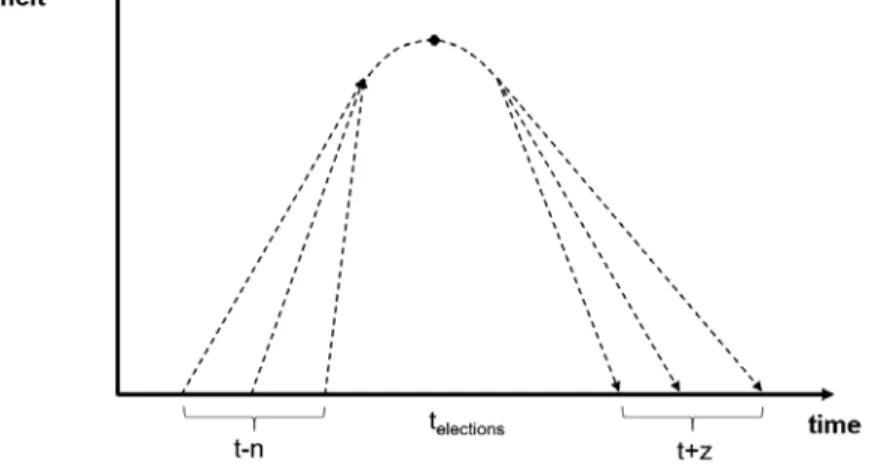
Figure 1 presents the possible course of a PBC. The literature usually focuses on examining the cycles in the year of elections or a year before them, i.e. n equals one or zero. Arguably, the “recovery” is individual to each government or economy. Some scholars tend to find significant effects of reaching budget surpluses a year after elections, i.e. z is one and a line goes to negative values in Figure 1.1
Shi – Svensson (2002) observed that the second generation of the models is based on adverse selection where signalling behaviour is important. Politicians demonstrate to voters that they are competent and worth being elected. The third generation of the models is built on the assumption of moral hazard. In this sense, political competence can be attributed to the usage of various policy instruments.
The game results in government’s excessive effort to operate the instruments that, in turn, leads to increased budget deficits (Mink – de Haan 2006).
Most of the previous studies have assumed that the effects of PBCs are identi- cal in each country. However, this assumption is probably not valid. The research has shifted and currently examines whether the PBCs exist in each case and how the cycles differ between diverse countries. This paper uses a similar approach.
Haan – Klomp (2013) discussed the heterogeneous influence of factors, such as institutional quality, level of development of economies, age and level of democ- racy, electoral rules and the form of the government, transparency of the politi- cal process, presence of checks and balances, and fiscal rules. For instance, Shi
1 For example, see Gregor (2016).
Figure 1. A possible development of a political budget cycle
– Svensson (2006) presented evidence that the strength of the PBCs is higher in developing countries.
1.2. Political budget cycles in the EU
Researchers tend to find PBCs in the EU, however, in some regard, the evidence is contradictory. For example, the literature disputes whether the cycles exist only in the case of young democracies, as presented by Brender – Drazen (2005), or even in the “more established” democracies. Shi – Svensson (2006), Mink – de Haan (2006) and de Haan – Klomp (2013) found evidence supporting the latter.
Naturally, researchers started to collect information on important characteristics that coincide with the PBCs or even cause them. Ademmer – Dreher (2016) are of the opinion that a powerful press is needed in order to eradicate the PBCs in the EU. Efthyvoulou (2012) claimed that the PBCs are larger and statistically more robust in the Eurozone countries than in the countries that have not yet adopted the euro. Donahue – Warin (2007) explored effects of supra-national fiscal rules and they do not consider them effective. Dolezalova (2011) supported the view that the openness of democracy is the most important characteristic in relation to the effective behaviour of governments. Bayar – Smeets (2009) concluded that political fragmentation does not play a big role in government deficits, while partisan behaviour has a weak effect. Their research also showed that the stabil- ity of the government has a significantly negative impact on the size of a budget deficit. It is clear that the researchers prefer focusing on one characteristic, which, they argue, is the key. But the euro or the openness to democracy, possibly, has no direct connection to the existence of the PBCs.
2. EVIDENCE ON POLITICAL BUDGET CYCLES IN THE EU
2.1. Theoretical framework
The primary motivation of this research is to verify a hypothesis that the PBCs exist throughout the EU. Furthermore, I will identify basic country characteristics that correlate to the existence of the PBCs. I use panel data for the EU member states; therefore, I will also assume that the economic outcomes of each country may differ. Otherwise, the presence of the country-specific effects in a stand- ard panel-data setting would bias the standard ordinary least squares estimator (OLS).
The next step is a consideration whereby to use the prominent fixed-effects (FE) estimation, which is conservative and theoretically more suitable than the random-effects technique. Due to the obvious difficulties in the estimation of complicated explanatory variables such as the budget balances in relation to GDP, I turn to the usage of autoregressive (AR) processes that help explain the possible inertia, and their inclusion is appropriate when dealing with a highly persistent data series. Nickel (1981) demonstrated that the AR processes cause endogeneity, rendering the FE estimation to be biased in the finite-sample properties. There- fore, the focus needs to turn to a dynamic panel data estimation, which addresses the problem.
A popular tool is the so-called difference GMM estimator,2 proposed by Arel- lano – Bond (1991). In a nutshell, it is used for highly persistent data series with a large number of observations within a limited time-span, which include AR processes of the dependent variable. The estimation technique allows to include independent variables that are not strictly exogenous, i.e. they are correlated to the past and current realisations of the error term. Furthermore, the estimation allows for fixed effects, heteroscedasticity and autocorrelation within individuals (Roodman 2009). The panel specification can take the following form:
, , 1 , ,
1
,
N
i t j i t j i t i i t
j
Y αY β X μ ε
where Yi,t is the outcome of interest for individual i and time t, the summation term represents the lags of the Yi,t , Xi,t is a set of regressors that may include past val- ues, μi is a time-invariant unobservable and εi,t is a time-varying unobservable .
Furthermore, the estimator solves endogeneity problems of the correlation be- tween unobservable and observable variables by using instrumental variables.
Arellano – Bond (1991) suggest the inclusion of second lags of the dependent variable and all the feasible lags thereafter. This gives a constantly expanding number of instruments as the time period progresses.
For instance, five time periods can yield a set of six instruments in the case of a single variable, Y (and more instruments as the time-span tends to infinity):
2 In the context of panel data and unobserved heterogeneity, the within (demeaning) transforma- tion is usually applied, as in the case of one-way fixed-effects models. Alternatively, one can consider taking the first differences. The GMM approach employs the latter solution.
t → n Yt–1, Yt–2, Yt–3,… Yt–2,
…
t = 5 Yt–1, Yt–2, Yt–3 (S.1)
t = 4 Yt–1, Yt–2
t = 3 Yt–1
Later, Arellano – Bover (1995) proposed an approach, which was further de- veloped by Blundell – Bond (1998), thereby creating the so-called system-GMM estimator. The motivation was simple, if a variable is close to a random walk, then the difference GMM performs poorly. This is because the past levels convey little information about future changes, so untransformed lags are weak instruments for transformed variables (Roodman 2009). In other words, where Arellano – Bond instruments have differences with levels, Blundell – Bond instruments have levels with differences. The system-GMM estimator uses lagged differences as instruments for equations in levels, in addition to lagged levels as instruments for equations in first differences. The technique is proved to be asymptotically more efficient than the first approach. Thus, I employ a two-step system-GMM estima- tion, which is found to be more efficient than the one-step estimator, although both are asymptotically equivalent (Roodman 2015). In addition, the standard errors of the two-step estimator suffer from a downward bias. Windmeijer (2005) was able to correct this bias, therefore, I use his corrected standard errors.
2.2. The problem of too many instruments and its solution
Apparently, the estimation may easily suffer from instrument proliferation which can overfit the endogenous variables and fail to eliminate their endogenous com- ponents. Moreover, it could bias the Hansen test that is used to identify this prob- lem.3 The usual rule of thumb is to have fewer instruments as compared to panel groups. Therefore, the researchers usually limit the total number of instruments.
Initially, a wise choice of variables can help reduce the instrument count. In this regard, I do not use a full set of time effects, instead, the models incorporate
3 Roodman (2009) claims that researchers should avoid suspiciously high values of the Hansen test statistic. When the number of instruments is very high, the Hansen’s p-value usually shows 1. I have avoided such results in the estimations.
decade dummy variables capturing each decade instead of each time period.4 The decade form of time effects can also be found in the works of Veiga et al.
(2017). However, the strategy alone does not sufficiently reduce the number of instruments, the solution must also be technical. The instrument matrix can be collapsed5 or one can use a fixed number of lags. The literature, considering the PBCs, usually limits the number of instruments by incorporating only second lags of the endogenous variables. However, I do not find the approach convinc- ing because a lot of information is lost, and the usage of good instruments is especially important. Mehrhoff (2009) suggests employing the PCA in limiting the total number of instruments.6 Therefore, I adopt this solution to the problem, besides collapsing the instrument matrix, and, hopefully, enhancing the estima- tion efficiency. The PCA is frequently used with a variety of other statistical tech- niques, among which is a regression analysis.7 The strategy has the advantage of being purely data-driven and, hence, being a less arbitrary choice for instrument reduction (Ferreira et al. 2014). The main idea of the method is to reduce the di- mensionality of a data set, consisting of a large number of interrelated variables, while retaining as much as possible of the variation present in it. This is done by transforming to a new set of variables, called the principal components, which are uncorrelated and ordered, such that the first few retain most of the variation present in all the original variables (Jolliffe 2002). In other words, it effectively reduces the original data dimension while maintaining as much information as possible. In this case, I apply the PCA to the instrument set as it extracts the larg- est eigenvalues of the estimated covariance matrix (Mehrhoff 2009). As a result, the instrument matrix should contain more precise information and I hope to get more accurate estimates that are not biased by a subjective approach to the re- duction of instruments. The concern about the quality of estimates is especially important when it comes to working with instruments.
4 The time effects help fulfil the assumption that the observations are independent among the groups. Moreover, their inclusion aids with potential non-stationarity. Nevertheless, the vari- ables exhibit mostly stationary properties and the number of groups is higher than the time pe- riod, making the problem less severe. The problem of non-stationarity is usually not discussed in terms of the used estimation technique and the model specification.
5 This makes the instrument count linear rather than quadratic in time. See Roodman (2009) for a more detailed explanation.
6 The Principal Component Analysis is integrated in the xtabond2 command in Stata.
7 For a detailed explanation, please refer to Jackson (1991) or Jolliffe (2002).
2.3. Further theoretical considerations
Furthermore, I will discuss the specifications and data choice in the context of other researchers’ findings. Streb et. al. (2012) argue that the use of annual data underestimates the effect of PBCs. The cycles are possibly more observable in the quarterly series. However, in the case of the EU, there is not enough data to perform such analysis. It would also restrict the number of variables, groups (countries), and the time-span; thus, making the analysis potentially less robust and less valuable. Nevertheless, capturing the PBCs in the context of annual data may serve as a solid evidence of their existence for the same reason (the coefficients may be lower, and the relationship could be arguably more diffi- cult to obtain). In addition, the literature widely discusses the prospects of an endogenous electoral timing. I decided not to treat the variable ELEC_effect as endogenous because of four main reasons. 1) Brender – Drazen (2005), followed by Ademmer – Dreher (2016), claimed that there exists neither a clear theoretical argument nor empirical evidence that it substantially alters the results. 2) Persson – Tabellini (2003) argued that the election dates may be correlated to the eco- nomic cycle. However, these prospective problems are addressed by inclusion of the income shocks among the controls. All the specifications in this paper contain both the GDP growth and the growth of real adjusted disposable income. 3) Shi – Svensson (2006) claimed that crises or social unrests may introduce endogene- ity if they are not included in the regressions. The specifications in my analysis include decade (time) effects. At the same time, the authors examined developing countries and found that the EU member states did not suffer from substantial un- rests, as was the case of less developed economies in the examined time period.
4) Finally, Efthyvoulou (2012) assumed endogenous election timing in the EU and found that the presence of PBCs is not driven by strategically timed elections but, paradoxically, the fiscal manipulation is stronger when the election date is exogenously fixed by the law.
Regarding the selection of control variables, I treat GDP and income vari- ables as endogenous. The effect of population and changes in government can be considered as exogenous. The latter is possibly more debatable. However, I also do not see any strong theoretical argument that could prove significant bias in the results. In the context of augmented models, variables such as tax burden do not enter the estimation directly; they are used only for creating the groups of countries.
2.4. Empirical specifi cations
In order to capture the relationship between budget balances and elections, I em- ploy two sets of widely used panel-model specifications based on the proposition of Shi – Svensson (2002, 2006) and Persson – Tabellini (2003). The baseline model takes the following form:
2
, , 1 , 2 ,
1
3 , ,
_
1. _
i t j i t j i t i t
j
i t i i t
BUDGET BUDGET X GDP growth
L ELE effect
α β β
β μ ε
(M.1)where BUDGETi,t is a type of budget balance as a share on the GDP measure in country i and year t, Xi,t is a vector of control variables, GDP_ growthi,t is the growth rate of GDP, ELE_ effecti,t is the key (lagged) electoral dummy variable representing elections taking place, μi are unobserved country-specific effects and εi,τ is an i.i.d. error term. I use two types of the independent variables, first is the standard budget balance to GDP ratio (budget_exp_gdp), and the second is a struc- tural budget balance in relation to potential GDP (str_budget_exp_pt_gdp). The set of control variables consists of a change in the real adjusted gross disposable income per capita8 (r_adj_g_disp_inc_pc_chng), number of changes in govern- ment per year (gov_chan), share of working population’s ages between 15 to 64 to elderly people ageing 65+ (pop_15_64 / 65), and specific decade (time) effects.
The variables capture both the voter (demand) and the executive (supply) side, which motivates the fiscal outcomes together with the specific decade effects.9
Furthermore, I use an augmented model to get estimates for sub-samples of countries. This enables to explore the fragmentation within the EU and trace the characteristics that correlate with the existence of PBCs. The augmented model equation is as follows:
2
, , 1 , 2 ,
1
3 , 4 , , 5 , ,
_ _ _
1 (1 1 ) 1. _ 1
i t j i t j i t i t
j
i t i t i t i t i i t
STR BUDGET STR BUDGET X GDP growth
Group Group L ELE effect Group
α β β
β β β μ ε
(Μ.2)8 Some authors, for example, Shi – Svensson (2006) use a logarithm of real GDP per capita.
Nevertheless, as Janku (2016) shows, the use of the variable along with the standard GDP growth seems problematic due to the nearly perfect correlation between the two variables.
Therefore, I choose a different approach by using a more precise measure of real wealth per capita – real adjusted disposable income.
9 I do not employ a full set of time dummy variables in order to obtain unbiased results regard- ing the estimation technique. It is explained in detail in the previous chapter.
The specification follows the baseline model (see the text below M.1), but it features three notable differences. 1) I use only the structural budget balance to potential GDP as the dependent variable. I argue that a structural budget measure is more fitting for the analysis as it captures the true motivations of fiscal policies more precisely. In addition, it helps weaken the overly-strong correlations with the explanatory set of variables, such as GDP growth. 2) The election dummy ELEC_effect is multiplied by two dummy variables representing the opposite groups of countries. Thus, it becomes possible to get different estimates of the electoral effects on the budget balances for individual groups of states. The step needs to be complemented by adding the group dummy variable Group1 sepa- rately, to allow for differences between the group intercepts (Wright 1976). The election dummy does not need to be added independently as the group dummy variables are mutually exclusive (Brambor et al. 2006). 3) I introduce a control variable gdp_var that captures the cross-country differences in PBCs by subtract- ing the average GDP growth of one group from the opposite group of countries.
In other words, it lets the output growth differ across the sub-samples. I follow Efthyvoulou (2012) who argues that this strategy will ensure that the estima- tions do not draw misleading inferences regarding the cross-country variations of PBCs, which may be driven by distinct levels of economic growth across various country groups. Other characteristics are the same as in the baseline model (M.1) to ensure consistency.
Initially, the system-GMM estimation requires to set types to the variables with regard to instrument creation. I treat budget_exp_gdp, str_budget_exp_pt_gdp, gdp_growth, and r_adj_g_disp_inc_pc_chng as endogenous variables; therefore, I use two-and-more-period lagged levels for the differenced equation, and one- period lagged difference of these variables for the level equation as instruments.
The dummy variables and other indicators are treated as exogenous and are in- strumented by themselves in the differenced equation.
2.5. Data
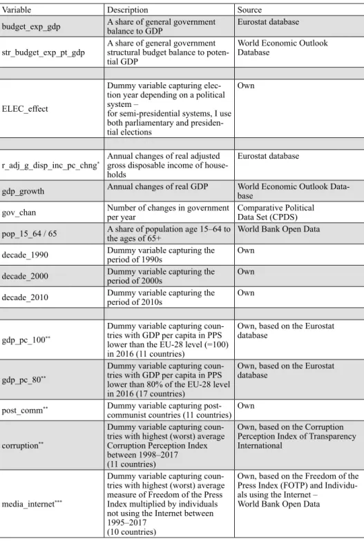
I use annual panel data of 1995–2016 for all 28 countries of the EU. Some values are missing, therefore, I work with an unbalanced panel. Table 1 contains a sum- mary of the variables used in the models. Descriptive statistics are available in Appendix .
With regard to the identification of country characteristics that correlate to the existence of PBCs, I need to specify a “cut-off point”, which will be used to sepa- rate the countries, based on their distinct performance in various macroeconomic factors. The initial target was to use a relatively representative sample of 10 out
Table 1. Summary of key variables
Variable Description Source
budget_exp_gdp A share of general government
balance to GDP Eurostat database
str_budget_exp_pt_gdp A share of general government structural budget balance to poten- tial GDP
World Economic Outlook Database
ELEC_effect
Dummy variable capturing elec- tion year depending on a political system –
for semi-presidential systems, I use both parliamentary and presiden- tial elections
Own
r_adj_g_disp_inc_pc_chng* Annual changes of real adjusted gross disposable income of house- holds
Eurostat database
gdp_growth Annual changes of real GDP World Economic Outlook Data- base
gov_chan Number of changes in government
per year Comparative Political
Data Set (CPDS) pop_15_64 / 65 A share of population age 15–64 to
the ages of 65+ World Bank Open Data
decade_1990 Dummy variable capturing the
period of 1990s Own
decade_2000 Dummy variable capturing the
period of 2000s Own
decade_2010 Dummy variable capturing the
period of 2010s Own
gdp_pc_100**
Dummy variable capturing coun- tries with GDP per capita in PPS lower than the EU-28 level (=100) in 2016 (11 countries)
Own, based on the Eurostat database
gdp_pc_80**
Dummy variable capturing coun- tries with GDP per capita in PPS lower than 80% of the EU-28 level in 2016 (17 countries)
Own, based on the Eurostat database
post_comm** Dummy variable capturing post- communist countries (11 countries) Own
corruption**
Dummy variable capturing coun- tries with highest (worst) average Corruption Perception Index between 1998–2017 (11 countries)
Own, based on the Corruption Perception Index of Transparency International
media_internet***
Dummy variable capturing coun- tries with highest (worst) average measure of Freedom of the Press Index multiplied by individuals not using the Internet between 1995–2017
(10 countries)
Own, based on the Freedom of the Press Index (FOTP) and Individu- als using the Internet –
World Bank Open Data
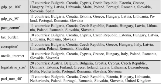
of 28 countries (36% – which is considered an appropriate size) for each dummy variable. However, in some cases, I ran into a problem as there were notable gaps between some groups of countries in the extremities. Therefore, I decided not to stick to an arbitrary sample size and specified the sample of countries individu- ally, for each of the considered characteristics. A list of the countries specified in each group is depicted in Table 2 below. Regarding the legislative_size variable,
Table 1. continued
Variable Description Source
tax_burden
Dummy variable capturing coun- tries with the lowest average Tax Burden Index between 1995–2017 (10 countries)
Own, based on the Tax Burden Index of the IEF (Heritage Foun- dation)
legislative_size**
Dummy variable capturing countries with a lower number of average directly elected legislative officials – between 1995–2017 (20 countries)
Own, based on the Electoral Sys- tem Design Database – Average of legislative size – directly elected measure (International IDEA)
parl_turn_40**
Dummy variable capturing coun- tries with lowest average voter turnout depending on a political system (see L1. ELEC_effect) between 1995–2017 (13 countries)
Own, based on the Voter Turn- out Database – Average of voter turnout – depending on a political system (International IDEA)
Notes: * Due to data unavailability, I used changes of real gross disposable income of households (not adjusted) in the case of Malta. ** The initial target was to use 10 countries in each group, however, in these cases, I had to change it because of other thresholds or the notable gaps between groups of countries. Regarding the legisla- tive_size variable, I found the election effect to be significant only in a larger sample of countries. *** The inclu- sion of this variable is inspired by Ademmer – Dreher (2016), who used the same procedure.
Table 2. Overview of countries represented in the key group dummy variables
Variable Selected countries
gdp_pc_100* 17 countries: Bulgaria, Croatia, Cyprus, Czech Republic, Estonia, Greece, Hungary, Italy, Latvia, Lithuania, Malta, Poland, Portugal, Romania, Slovakia, Slovenia, Spain
gdp_pc_80* 11 countries: Bulgaria, Croatia, Estonia, Greece, Hungary, Latvia, Lithuania, Po- land, Portugal, Romania, Slovakia
post_comm* 11 countries: Bulgaria, Croatia, Czech Republic, Estonia, Hungary, Latvia, Lithua- nia, Poland, Romania, Slovakia, Slovenia
tax_burden 10 countries: Bulgaria, Croatia, Cyprus, Czech Republic, Estonia, Hungary, Latvia, Lithuania, Romania, Slovakia
corruption* 11 countries: Bulgaria, Croatia, Czech Republic, Greece, Hungary, Italy, Latvia, Lithuania, Poland, Romania, Slovakia
media_internet 10 countries: Bulgaria, Croatia, Cyprus, Greece, Hungary, Italy, Poland, Romania, Slovakia, Slovenia
legislative_size* 20 countries: Austria, Belgium, Bulgaria, Croatia, Cyprus, Czech Republic, Denmark, Estonia, Finland, Greece, Ireland, Latvia, Lithuania, Luxembourg, Malta, Netherlands, Portugal, Romania, Slovakia, Slovenia
parl_turn_40* 13 countries: Bulgaria, Croatia, Czech Republic, Estonia, Hungary, Lithuania, Netherlands, Poland, Portugal, Romania, Slovakia, Slovenia, United Kingdom
I found the electoral effect to be significant only in a larger sample of countries, making it less robust.
2.6. Existence of political budget cycles in the EU
The aim of this research is to assess whether the EU countries suffer from sig- nificant increases of budget deficits prior to the parliamentary or presidential elections.10 Table 3 presents the results of the analysis. The models use two lags of the dependent variables and time effects represented by decade dummy vari- ables. Neither estimated models suffer from AR-2 autocorrelation or invalid in- struments as demonstrated by the Arellano – Bond (A-B) and the Hansen tests.
In addition, the number of instruments has been brought down by the PCA and is lower than the number of groups.11 The key variable is the first lag of the ELEC_effect representing elections based on the political system of a country.12 Therefore, the analysis explores the effects of elections on budget deficits a year before the elections are held. I estimate the models for both the standard budget balance to the GDP and the structural budget balance to the potential GDP ratios.
The two indicators exhibit inertia; the inclusion of lags and the estimator choice seems appropriate. The annual growth of GDP (gdp_growth) is significant only in the case of the standard budget balance to GDP ratio, the coefficient is positive which is in line with economic theory. Logically, the relation of structural budget balance to GDP growth should be weaker, and the model also confirms the fact.
The number of changes in the governments per year (gov_chan) is significant in both cases and negatively affects the budget balances. One possible explanation is that there is high competition between participating political parties, which leads to higher budget deficits. The second explanation could be that the ruling parties, that are experiencing instabilities, are more motivated to run deficits.
Possibly, they need to improve their weakened public image in the short run to win the upcoming elections.
The magnitudes of the key dummy variables (L1. ELEC_effect), concerning the budget deficits a year before the election year, are in a credible range of –0.41 to –0.50 percentage points. According to my presumptions, the electoral effect is weaker in the case of the structural budget balance to potential GDP ratio. The hy-
10 I treat each case carefully and distinguish between the electoral systems. Accordingly, I adjust the key electoral dummy variable. I use both parliamentary and presidential elections for the semi-presidential systems.
11 Therefore, the Hansen test values are not excessively high, making them robust. The issue was explained in the chapter concerning methodology.
12 See Table 1 for a detailed explanation.
Table 3. Existence of political budget cycles in the EU
Model (1) Two-step system GMM (2) Two-step system GMM
Dependent variable Budget balance to GDP (budget_exp_gdp)
Structural budget balance to potential GDP (str_budget_exp_pt_gdp)
L1. dependent variable 0.630***
(0.125) 0.862***
(0.074)
L2. dependent variable –0.0872
(0.098) –0.113
(0.076)
L1. ELEC_effect –0.496**
(0.221) –0.414**
(0.174)
gdp_growth 0.319***
(0.109) 0.126
(0.083) r_adj_g_disp_inc_pc_chng 0.0833
(0.152) –0.122
(0.093)
gov_chan –0.445***
(0.134) –0.277**
(0.109)
pop_15_64 / 65 –0.943
(0.822) –0.982
(0.585)
Time (decade) effects Yes Yes
A-B test (AR-2)a 0.964
(0.335) 0.855
(0.393)
Hansen testb 12.08
(0.280) 11.31
(0.334)
Number of instruments 20 20
K-M-O measurec 0.872 0.864
Components explan. powerd 0.740 0.747
Number of countries 28 28
Number of observations 513 464
Notes: Robust standard errors with finite-sample correction developed by Windmeijer (2005) are in parentheses, t-statistics were used; * p < 0.1, ** p < 0.05, *** p < 0.01.
Instruments used in the system GMM regression are lagged levels (two and more periods) of the dependent variable and the variables gdp_growth and r_adj_g_disp_inc_pc_chng for the differenced equation, and lagged difference (one period) of these variables for the level equation. The dummy and the other variables are treated as being exogenous and are instrumented by themselves in the differenced equation.
In order to limit the number of instruments, the GMM-type instrument matrix was collapsed, Principal Com- ponent Analysis was employed on the GMM-type instruments, and decade dummy variables were used instead of the full set of time effects.
a Reports the Arellano – Bond test for second-order serial correlation of the differenced residuals (p-values in parentheses).
b Reports the Hansen test for over-identifying restrictions (p-values in parentheses).
c Kaiser – Meyer – Olkin measure of sampling adequacy.
d Portion of variance explained by the components.
pothesis that PBCs exist in the EU is confirmed. In addition, there is possible evi- dence that PBCs are significant in (t-1), i.e. in a year before the election year.13
Moreover, I explore the existence of the PBCs in terms of the EU elections and various referenda, but the results are inconsistent and insignificant. Arguably, the cycles do not exist in these cases. Furthermore, the presumption is that the use of the structural budget balance variable is more fitting as mentioned in the previous section, so I use it exclusively in the subsequent analysis.
2.7. Existence of political budget cycles in sub-samples of countries
The second part of the analysis is to explore a fragmentation in the EU in terms of the existence of the PBCs, I try to find countries’ characteristics that correlate with the PBCs. I investigate more than 30 associations that could be fitting.14 These include the level of GDP, indebtedness, total government expenditures, tax burden, trade openness, common currency, economic freedom, fiscal rules, geo- graphical location, political ideology, electoral systems, electoral voting systems, the role of media, corruption, and educational attainment of citizens. It becomes possible to identify PBCs in eight groups of the EU countries. According to the analysis, the characteristics that possibly correlate with the existence of strong PBCs in the EU are as follows:
GDP per capita lower than 100% of the EU-28
GDP per capita lower than 80% of the EU-28
Post-communist background
Comparatively lower overall tax-burden
Comparatively higher levels of perceived corruption
Comparatively lower levels of media freedom and internet usage
Comparatively lower number of directly voted legislative officials
Parliamentary voter turnout lower than 40%
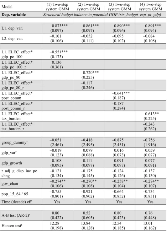
Tables 4 and 5 present the results of the models in the same order. In this case, I present the augmented models with the electoral dummy variable appearing two times in each case, capturing both subsamples of countries divided by the selected characteristics, mentioned above.15 These variables are then multiplied by the lagged electoral dummy (L1. ELEC_effect) to get estimates of the possible
13 The majority of studies concerning PBCs examine the electoral effects in the year of elections.
I use a first lag of that variable instead.
14 According to my knowledge, a broad analysis of this kind has not yet been conducted.
15 Each augmented model contains two groups of countries. For example, the first model is working with a group of countries whose GDP per capita in PPP is higher or lower than 100%
of the EU-28.
existence of PBCs in each group. As noted, I use the structural budget balance in relation to the potential GDP ratio as a dependent variable, which is found to be more fitting.
The first lags of the dependent variable are again both statistically and eco- nomically significant, therefore, the inclusion of the AR processes and the es- timation techniques seem appropriate. All the estimated models do not exhibit autocorrelation or invalid instruments, which is indicated by the A-B and the Hansen test values. Furthermore, the instrument count has been brought down by the PCA again, making it lower than the number of the examined countries and keeping the Hansen test values in a relatively safe range.
The new variable (gdp_var) used in the augmented models, which captures the differences in the average GDP growth between sub-samples, is found to be significant in one model, possibly weakening the effects of the GDP growth (gdp_growth). The government changes indicator (gov_chan) is significant and again negative in all the models, demonstrating the possible effects of political competition or the instability of ruling parties, which was explained in the previ- ous chapter. The effect of a change in the real adjusted gross disposable income (r_adj_g_disp_inc_pc_chng) is found to be significant in one model, negatively affecting the structural budget balance. Possibly, when voters’ incomes increase, the incentives and the returns from the rising expenditures, a year before the elec- tion year, weaken. Logically, there should be some form of a trade-off. The vari- able ratio of working population to elderly population (pop_15_64 / 65) is found to be significant and its effect is negative in one model as well. Theoretically, a higher number of potential voters could mean higher incentives for PBCs or I could argue that the strength of lobby groups increases with the growing majority of voters, for whom it is more difficult to reach a consensus.
Tables 4 and 5 show that the effects of the main electoral variables (multiplied by each sub-sample) are statistically and economically significant, ranging from –0.49 to –0.76 percentage points. Regarding the group characteristics, I cannot prove direct causality between them and the PBCs because the selected variables do not exhibit significance as explanatory variables for the full sample. Possibly, some form of threshold exists and working with sub-samples may help under- stand the situation.
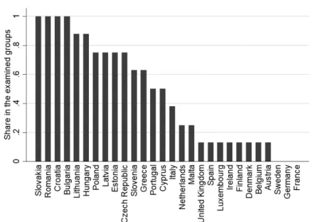
I find evidence that the results are driven by the countries of Central and Eastern Europe. Four countries are represented in each of the examined groups: Slovakia, Romania, Croatia, and Bulgaria. Moreover, six more countries are included in the groups with shares equal to or higher than 75%; these are: Lithuania, Hun- gary, Poland, Latvia, Estonia, and the Czech Republic. Possibly, and these states exhibit the strongest PBCs in the EU. On the other hand, states such as France, Germany, and Sweden (along with 10 other countries that exhibit a share that is
Table 4. Selected characteristics that correlate with the political budget cycles (A)
Model (1) Two-step
system GMM (2) Two-step
system GMM (3) Two-step
system GMM (4) Two-step system GMM Dep. variable Structural budget balance to potential GDP (str_budget_exp_pt_gdp)
L1. dep. var. 0.873***
(0.097) 0.861***
(0.097) 0.890***
(0.096) 0.891***
(0.094)
L2. dep. var. –0.101
(0.106) –0.052
(0.111) –0.095
(0.102) –0.084
(0.108) L1. ELEC_effect*
gdp_pc_100 –0.551***
(0.173) L1. ELEC_effect*
gdp_pc_100_r 0.136
(0.361) L1. ELEC_effect*
gdp_pc_80 –0.720***
(0.225) L1. ELEC_effect*
gdp_pc_80_r –0.117
(0.246) L1. ELEC_effect*
post_comm –0.641***
(0.187) L1. ELEC_effect*
post_comm_r –0.187
(0.284) L1. ELEC_effect*
tax_burden –0.613**
(0.225) L1. ELEC_effect*
tax_burden_r –0.243
(0.262)
group_dummy* –0.051
(2.461) –0.418
(2.495) –0.875
(2.451) –0.756
(1.916)
gdp_var* –0.019
(0.123) 0.079
(0.088) 0.016
(0.073) 0.059
(0.077)
gdp_growth 0.108
(0.095) 0.111
(0.097) –0.091
(0.097) 0.077
(0.091) r_adj_g_disp_inc_pc_
chng –0.121
(0.134) –0.175
(0.145) –0.124
(0.126) –0.137
(0.130)
gov_chan –0.274**
(0.106) –0.270**
(0.108) –0.258**
(0.104) –0.274**
(0.107)
pop_15_64 / 65 –0.755
(0.801) –0.921
(0.902) –0.664
(0.852) –0.734
(0.831)
Time (decade) eff. Yes Yes Yes Yes
A-B test (AR-2)a 0.80
(0.422) 0.52
(0.605) 0.80
(0.423) 0.76
(0.448)
Hansen testb 12.28
(0.198) 13.84
(0.128) 12.54
(0.185) 13.01
(0.162)
Table 4. continued
Model (1) Two-step
system GMM (2) Two-step
system GMM (3) Two-step
system GMM (4) Two-step system GMM
No. instruments 22 22 22 22
K-M-O measurec 0.864 0.864 0.864 0.864
Comp. expl. pwr.d 0.747 0.747 0.747 0.747
No. countries 28 28 28 28
No. observations 464 464 464 464
Notes: See Table 3.
Suffixes _r of the election*group dummy variables represent the opposite sample of countries of each group;
L1. ELEC_effect * (1-original group dummy).
* In order to save space, the differences in average real GDP growth between the groups (gdp_var) and the separate group dummy variables (group_dummy) are reported in the single rows, even though they belong to separate rows (different variable names) – they should form a cascade, same as in the case of the election*group dummy variables.
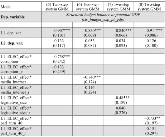
Table 5. Selected characteristics that correlate with the political budget cycles (B)
Model (5) Two-step
system GMM (6) Two-step
system GMM (7) Two-step
system GMM (8) Two-step system GMM Dep. variable Structural budget balance to potential GDP
(str_budget_exp_pt_gdp)
L1. dep. var. 0.907***
(0.101) 0.850***
(0.069) 0.840***
(0.066) 0.911***
(0.086)
L2. dep. var. –0.133
(0.117) –0.053
(0.087) –0.034
(0.093) –0.126
(0.100) L1. ELEC_effect*
corruption –0.758***
(0.242) L1. ELEC_effect*
corruption _r –0.133
(0.249) L1. ELEC_effect*
media_internet –0.740***
(0.174) L1. ELEC_effect*
media_internet_r 0.116
(0.224) L1. ELEC_effect*
legislative_size –0.485**
(0.189) L1. ELEC_effect*
legislative_size_r 0.040
(0.276) L1. ELEC_effect*
parl_turn_40 –0.733**
(0.197) L1. ELEC_effect*
parl_turn_40_r –0.151
(0.297)
equal to or less than 25%) do not show notable signs of PBCs according to their representation in the groups. The results are shown in Figure 2. As opposed to Efthyvoulou (2012), I do not find significant electoral effects in the euro area. 16 Furthermore, the most-indebted Southern countries do not show significant ef- fects either. According to the representation in the 8 groups, their cycles’ strengths are rather low to mediocre.
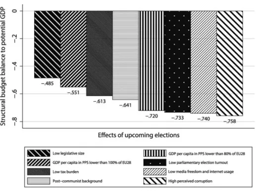
Furthermore, Figure 3 shows that the groups of countries with the compara- tively higher perceived levels of corruption, lower media freedom, lower GDP
16 Therefore, I do not present empirical results for this group of states.
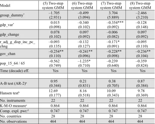
Table 5. continued
Model (5) Two-step
system GMM (6) Two-step
system GMM (7) Two-step
system GMM (8) Two-step system GMM
group_dummy* –1.705
(2.931) –0.499
(3.094) 3.704
(5.889) –2.466
(3.210)
gdp_var* 0.015
(0.098) –0.340
(0.102) –0.354***
(0.092) –0.128
(0.148)
gdp_change 0.078
(0.102) 0.097
(0.092) –0.006
(0.082) 0.097
(0.092) r_adj_g_disp_inc_pc_
chng –0.093
(0.135) –0.132
(0.127) –0.171*
(0.091) –0.095
(0.110)
gov_chan –0.254**
(0.110) –0.241**
(0.096) –0.228**
(0.098) –0.236**
(0.104)
pop_15_64 / 65 –0.562
(0.749) –1.235*
(0.710) –0.239
(0.640) –0.359
(0.824)
Time (decade) eff. Yes Yes Yes Yes
A-B test (AR-2)a 0.95
(0.344) 0.21
(0.831) 0.38
(0.705) 0.87
(0.384)
Hansen testb 12.69
(0.177) 8.16
(0.518) 10.09
(0.343) 9.78
(0.369)
No. instruments 22 22 22 22
K-M-O measurec 0.864 0.864 0.864 0.864
Comp. expl. pwr.d 0.747 0.747 0.747 0.747
No. countries 28 28 28 28
No. observations 464 464 464 464
Notes: See Table 3.
Suffixes _r of the election*group dummy variables represent the opposite sample of countries of each group;
L1. ELEC_effect * (1-original group dummy).
* In order to save space, the differences in average real GDP growth between the groups (gdp_var) and the separate group dummy variables (group_dummy) are reported in the single rows, even though they belong to separate rows (different variable names) – they should form a cascade, same as in the case of the election*group dummy variables.
per capita, and lower parliamentary turnout show the strongest PBCs. The weak- est coefficient is recorded in the case of legislative size, i.e. comparatively lower number of directly elected legislative officials.
3. CONCLUSIONS
This research suggests that political budget cycles do exist in the EU. I have used data for 28 EU countries for the period of (1995–2016). In addition, I have found significant PBCs in a year before the election year (t–1), as opposed to a majority of other studies that examine the same period.
The estimates of this research have been enhanced by employing the Principal Component Analysis, which is reflected in the Hansen test, making the results more robust. The structural budget deficit related to potential GDP ratio rises by –0.41 percentage points a year before the election year while the standard budget deficit measure increases by –0.5 percentage points. The structural budget meas- ure seems more appropriate for the analysis, as it more effectively captures the true motivations of the fiscal policies.
The second segment of the analysis deals with the broad fragmentation of the EU in terms of the cycles. I have investigated more than 30 associations that could be fitting and presented eight characteristics correlating to strong PBCs
Figure 2. Shares of countries represented in the examined groups
– all of them being included in one analysis. To be more specific, the character- istics are as follows: GDP per capita lower than 100% of the EU-28, GDP per capita lower than 80% of the EU-28, post-communist background, comparatively lower overall tax-burden, comparatively higher levels of perceived corruption, comparatively lower levels of media freedom and internet usage, comparatively lower number of directly voted legislative officials, and a parliamentary voter turnout lower than 40%. The PBC coefficients range from –0.49 to –0.76 per- centage points. The groups of countries with the comparatively higher perceived corruption, lower media freedom, lower GDP per capita, and lower parliamentary turnout exhibit the strongest PBCs.
When I consider the representation of each EU country in these selected groups, I tend to find that the strongest cycles occur in the relatively new EU member countries of Central and Eastern Europe. The research could possibly be enhanced by using quarterly data, however, they are not available in the case of many indicators. Finally, I propose taking into consideration a higher number of characteristics and not relying on a sole aspect when explaining the heterogeneity of the PBCs in the EU.
Figure 3. Magnitudes of electoral effects based on various characteristics
REFERENCES
Ademmer, E. – Dreher, F. (2016): Constraining Political Budget Cycles: Media Strength and Fiscal Institutions in the Enlarged EU. Journal of Common Market Studies, 54(3): 508–524.
Arellano, M. – Bond, S. (1991): Some Tests of Specifi cation for Panel Data: Monte Carlo Evidence and an Application to Employment Equations. Review of Economic Studies, 58(2): 277–297.
Arellano, M. – Bover, O. (1995): Another Look at the Instrumental Variable Estimation of Error- Components Models. Journal of Econometrics, 68(1): 29–51.
Bayar, A. H. – Smeets, B. (2009): Economic, Political and Institutional Determinants of Budget Defi cits in the European Union. CESifo Working Paper Series, No. 2611.
Blundell, R. – Bond, S. (1998): Initial Conditions and Moment Restrictions in Dynamic Panel Data Models. Journal of Econometrics, 87(1): 115–143.
Brambor, T. – Clark, W. R. – Golder, M. (2006): Understanding Interaction Models: Improving Empirical Analyses. Political Analysis, 14(1): 63–82.
Brender, A. – Drazen, A. (2005): Political Budget Cycles in New versus Established Democracies.
Journal of Monetary Economics, 52(7): 1271–1295.
Brender, A. – Drazen, A. (2008): How do Budget Defi cits and Economic Growth Affect Re-Elec- tion Prospects? Evidence from a Large Cross-Section of Countries. American Economic Re- view, 98(1): 2203–2220.
De Haan, J. – Klomp, J. (2013): Conditional Political Budget Cycles: A Review of Recent Evi- dence. Public Choice, 157(3–4): 387–410.
Dolezalova, J. (2011): The Political-Budget Cycle in Countries of the European Union. Review of Economic Perspectives, 11(1): 12–36.
Donahue, K. – Warin, T. (2007): The Stability and Growth Pact: A European Answer to the Political Budget Cycle? Comparative European Politics, 5(4): 423–440.
Dubois, E. (2016): Political Business Cycles 40 Years after Nordhaus. Public Choice, 166(1–2): 235–
259.
Drazen, A. – Eslava, M. (2006): Pork Barrel Cycles. NBER Working Paper Series, No. 12190.
Efthyvoulou, G. (2012): Political Budget Cycles in the European Union and the Impact of Political Pressures. Public Choice, 153(3–4): 295–327.
Ferreira, F. H. G. – Lakner, C. – Lugo, M. A. – Ozler, B. (2014): Inequality of Opportunity and Economic Growth: A Cross-Country Analysis. World Bank: Policy Research Working Paper Series, No. 6915.
Institute of Political Science, University of Berne (2017): Comparative Political Data Set 1960–
2014.
Jackson, J. E. (1991): A User’s Guide to Principal Components. New York: John Wiley & Sons, Inc.
Janku, J. (2016): Podmineny politicko-rozpoctovy cyklus v zemich OECD (Conditional Political Budget Cycle in the OECD Countries). Politicka ekonomie, 64(1): 65–82.
Jolliffe, I. T. (2002): Principal Component Analysis. New York: Springer.
Karakas, M. (2012): Political Business Cycles in Turkey: Is It the Case? International Journal of Economic Sciences, I(2): 51–71.
Lami, E. – Kächelein, H. – Imami, D. (2014): A New View into Political Business Cycles: House- hold Behaviour in Albania. Acta Oeconomica, 64(1): 201–224.
Mehrhoff, J. (2009): A Solution to the Problem of Too Many Instruments in Dynamic Panel Data GMM. Bundesbank Series 1 Discussion Paper, No. 2009, 31.
Mink, M. – de Haan, J. (2006): Are There Political Budget Cycles in the Euro Area? European Union Politics, 7(2): 191–211.
Nickell, S. (1981): Biases in Dynamic Models with Fixed Effects. Econometrica, 49(6): 1417–
1426.
Nordhaus, W. D. (1975): The Political Business Cycle. Review of Economic Studies, 42(2): 169–
190.
Rogoff, K. – Sibert, A. (1988): Elections and Macroeconomic Policy Cycles. Review of Economic Studies, 55(1): 1–16.
Roodman, D. (2009): How to Do Xtabond2: An Introduction to Difference and System GMM in Stata. The Stata Journal, 9(1): 86–136.
Roodman, D. (2015): Xtabond2: Stata Module to Extend Xtabond Dynamic Panel Data Estimator.
Center for Global Development, Washington. https://econpapers.repec.org/software/bocbocode/
s435901.htm.
Shi, M. – Svensson, J. (2002): Conditional Political Budget Cycles. CEPR Discussion Paper, No.
3352.
Shi, M. – Svensson, J. (2006): Political Budget Cycles: Do They Differ Across Countries and Why?
Journal of Public Economics, 90(8–9): 1367–1389.
Streb, J. M. – Lema, D. – Garofalo, P. (2012): Temporal Aggregation in Political Budget Cycles.
Economia – Journal of the Latin American and Caribbean Economic Association, 13(1): 39–
78.
Tabellini, G. – Persson, T. (2003): Do Electoral Cycles Differ across Political Systems? IGIER Working Paper Series, No. 232.
Veiga, F. J. – Veiga, L. G. – Morozumi, A. (2017): Political Budget Cycles and Media Freedom.
Electoral Studies, 45(1): 88–99.
Windmeijer, F. (2005): A Finite Sample Correction for the Variance of Linear Effi cient Two-Step GMM Estimators. Journal of Econometrics, 126(1): 25–51.
Wright, G. (1976): Linear Models for Evaluating Conditional Relationships. American Journal of Political Science, 20(2): 349–373.