Acoustic Simulations based on FVM Solution of the Helmholtz Equation
Izabela Riečanová, Angela Handlovičová
Department of Mathematics and Descriptive Geometry
Faculty of Civil Engineering, Slovak University of Technology in Bratislava Radlinského 11, 810 05 Bratislava, Slovakia
riecanova@math.sk
Abstract: The main idea of the paper is an attempt to numerically simulate the data obtained by acoustic measurements. These measurements were performed in specialized acoustic laboratory. Their main idea was to study the reflection of different frequencies from boards with openings of various size and shape. The Finite volume method was used to make the simulations, where the Helmholtz equation is solved using the impedance boundary conditions. The results of the simulations are presented herein.
Keywords: measurement; Finite volume method; acoustic simulation; Fourier transform
1 Introduction - Acoustic Measurements
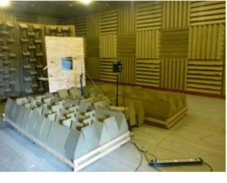
The main motivation of this work is to numerically simulate the values obtained by acoustic measurements. The measurements were performed in a specialized acoustic laboratory at the Faculty of Science at KU Leuven, in Belgium. The main idea is to study the reflection of different frequencies from boards with various openings. In Figure 1, there is the photo of one measuring experiment.
Figure 1 Photo of the measurement
As it is seen in the first figure, the measurements were performed in an anechoic room. Acoustically hard boards with openings of different size and shape were placed in the room and the impulse response measurements between the source and receiver were performed. The main focus was an analysis of sound reflection in frequency domain. Figure 2 shows simple scheme of the measurement.
Figure 2 Scheme of the measurement
At known positions of the space, the speaker and microphone were placed. These positions were also varying. Exponential sweep, containing all audible frequencies was used as a test signal, sent from the loudspeaker and recorded by microphone, and impulse response (will be presented in next section) was calculated.
The main assumption was that if there is full board placed in the room (as in the Figure 2), all frequencies with wavelength smaller than the size of the board will be reflected. In case of a board with opening, a part of the sound energy with higher frequency content won’t be reflected and will get through the panel, and the lower frequencies will fully reflect due to diffraction effects. If the opening is smaller, more of the frequencies are reflected. It is because the lower the frequency is, the bigger is its wavelength [9, 10]. When the frequency spectrum of the reflection was studied, our assumption was confirmed.
The main goal was the comparison of the data obtained from the measurements with numerical simulations implementing the Finite volume method.
2 Time Domain – Frequency Domain
This section describes the difference between the domains that the authors worked with and the conversion from one domain to the other.
The output from the acoustic measurements is the impulse response, which is shown in Figure 3.
Figure 3
Impulse response of the space
The measurement data is in the time domain, which means that the particular signal is studied considering time. In Figure 3, the horizontal axis is the time measured in seconds and the vertical axis is the acoustic pressure measured in Pascal. This record contains the information about the behavior of all frequencies during whole time. It can be clearly seen, that the first and biggest peak in the graph is the direct sound arriving at the microphone, and the following smaller peaks are the sound reflections arriving with a time delay.
The numerical methods which are used for our simulations, work in the frequency domain. That means that the signal is studied with respect to frequency – during the computations a constant frequency is considered. To decompose the function of time into the frequencies, the Fourier transform was used.
The Fourier transform of a function of time is complex valued function of frequency
. (1)
In the equation 1, is the frequency.
After the Fourier transform we obtain the data shown in the Figure 4.
On the horizontal axis the frequencies measured in Hertz. As can be seen there are also negative values of frequencies, which are the complex conjugate numbers of positive frequencies. These negative values were not important for us, but they are needed in case we would like to convert the data back to time domain.
Figure 4
Frequency spectrum of impulse response after Fourier transform
The Magnitude of the complex number is the amplitude of acoustic pressure.
Figure 5 shows this amplitude plotted on the logarithmic scale.
Figure 5
Amplitude of frequency domain signal plotted on logarithmic scale
We have taken the values from the frequency spectrum, which were used as the input data for the simulations. This was done by dividing the time-domain signal, so only a direct sound signal was obtained (Figure 6). We have applied the Fourier transform to this direct sound signal and computed data that was used in the program.
As the values in the frequency domain are variable (can be seen in Figure 4), it is not easy to choose the right frequency. If there is a Fourier transform done for either the direct sound or for the reflections, the frequency scaling is different so the interpolation had to be calculated. This approach may not be accurate, as the data oscillates, so this problem is left for further study.
Figure 6
Time domain signal – direct sound only
3 Helmholtz Equation
Numerical methods in the field of acoustics solve the Helmholtz equation
. (2)
Here is the Laplace operator, is the amplitude and is the wavenumber (number of radians per unit distance). The wavenumber is given by
(3) where is the angular frequency measured in radians per second, is the phase velocity measured in meters per second, and is the frequency.
The Helmholtz equation is related to the problems of steady-state oscillations. It is derived from the wave equation using the method of separating the variables, and it represents its time-independent form.
Because of its relation to the wave equation, the Helmholtz equation has use in various areas of physics, such as, electromagnetic radiation, elasticity or seismology. The main area of our interest is in acoustics. The algorithm based on the Finite volume method, presented later, is solving the Helmholtz equation.
4 Impedance Boundary Conditions
The boundary conditions which we mostly work with here are of the Robin type.
They are called the impedance boundary conditions [1, 5]
. (4)
Here is already mentioned amplitude, is imaginary unit and is the normal derivative. The function on the right hand side can be generally seen as the function of source. The parameter is the relative surface admittance. When this parameter is set to , this represents the simulation of acoustically hard wall with maximum energy reflected. When we set , it simulates the wall with maximal sound absorption, i.e. the free space. It is important to note, that if we do the calculation considering the inward normal, the sign is opposite . There must be mentioned that the Helmholtz equation with homogenous boundary conditions is an eigenvalue problem for the Laplacian [2]. When the situation where is the eigenvalue, the solution to the equation is not unique.
Moreover, its existence also depends on compatibility with the source function . This knowledge about the impedance boundary conditions, was implemented in our programs to simulate the aforementioned measurements.
5 Finite Volume Method
There are several numerical techniques for solving the Helmholtz equation and here we present the algorithm based on the Finite volume method [3, 4, 7, 8]. It is the method where the domain is discretized into cells called the finite volumes, which in our case were squares. The numerical solution , i.e. the numerical value of amplitude, is a piecewise constant function with one constant value on each cell. The values of unknown function are calculated at discrete points of mesh usually called the representative points in the form of algebraic equations.
Important feature of the method is the local conservativity of numerical fluxes, which means that the flux is conserved from one discretization cell to its neighbor.
Our case is three-dimensional, however we decided to simulate only the plane where the speaker and microphone were placed. Thus the problem reduces to two- dimensional which makes the computation easier and faster. The domain considered in the simulations was square, whereas its size was set to match the real situation.
After the volume discretization of the domain the grid of finite volumes is obtained ( is the number of discretizing points along one side of the domain). As the solution is complex valued function, it is in the form
. (5)
For better calculations we have worked with the following form of (2)
. (6)
The steps of the method are the integration of the Helmholtz equation (6) over the finite volume and applying the Green’s theorem about the relationship between line and double integral. Thus the following equation for the numerical solution was obtained
(7) where is particular finite volume, is its numerical solution on , and is the normal to the side of . When approximating the integrals, we used the fact that numerical solution is constant function on each cell. To the normal derivative the difference approximation was applied and the following equation was obtained
(8) where is the edge of the cell (| | is its length), is the size of cell, is the solution on the neighbor of particular finite volume, and denotes the distance between representative points of two adjacent finite volumes p and q (representative points were chosen the centers of finite volumes so the vector , connecting the points, is perpendicular to the edge). If we suppose that our finite volumes are squares so that , we get the following
. (9)
This equation (9) is valid for interior finite volumes. Thus we compute the equations for each cell for both, the real and imaginary part. The system of equations with matrix of size is obtained.
The equations for the finite volumes on the boundary or in the corner are slightly different, as these finite volumes have one or two exterior cells (Figure 7).
Figure 7
Representation of finite volume on the boundary
In these equations is the term denoting the numerical solution on exterior cell. As this value is not known, it was eliminated through the boundary conditions, which when written extra for real and imaginary part are
. (10)
This was obtained by substituting (5) into (4). Using the boundary conditions the following formula was derived
(11) which was used to solve this problem. h is the length of finite volume’s side. The created system of equation was solved by method of LU decomposition and once it was done, the solution of the acoustic pressure was calculated at each point of the domain.
6 Numerical Simulations
This section presents the numerical simulation of acoustic measurement using the described knowledge. The simulated particular measurement was shown in Fig. 1, with the board with square opening placed in anechoic room. The way the boundary conditions were prescribed is shown in Figure 8.
Figure 8
Representation of boundary conditions
For one finite volume on the boundary, the source function was prescribed with Dirichlet boundary conditions, where we put the values gained from the measurement. The relative surface admittance parameter was almost everywhere to simulate the free space. Only on part of domain’s right side it was to simulate the board.
From the measurements we have known the data at the point where the microphone was placed. To make the simulation more precise we wanted to know the values at the position of loudspeaker. To do this we used the knowledge about the sound intensity and its decrease with distance considering the spherical sound wave [6]
. (12)
Here is the sound intensity in known place measured in watt per square meter, and is decreased intensity in second place, where we want to know the value.
Then we used the formula about the sound intensity and its relation to the sound pressure
(13)
where is the sound pressure, is the density of air, and is the phase velocity. Using these formulas we have derived the new one, so we could increase the known measurement values and compute the data for the loudspeaker spot, which was used as Dirichlet boundary conditions.
As each frequency decreases differently when propagating in air, this way of amplifying the data might not be correct. Solution would be an improvement of the measurement, where there would be more than just one microphone placed in the space. This way we would own the data from more points so we could calibrate the values used for our simulations.
The following figures show the results of the simulations for the frequency of 436 Hz (for the value of wavenumber ). The value of real part of Dirichlet boundary conditions after recalculation using (12) and (13) was 4.772, and the value of imaginary part was 2.503. Figure 9 presents the real and imaginary part of the solution for and Figure 10 shows the amplitude of acoustic pressure (magnitude of complex number). The size of domain was .
Figure 9
Numerical solution for the frequency of 436 Hz, left – real part, right – imaginary part
Figure 10
Numerical solution of acoustic pressure amplitude for the frequency of 436 Hz
Next are the results where the domain was diminished, so that the microphone lies exactly in the left side of the domain. This way no data had to be recalculated. The Dirichlet boundary conditions were put along whole left side. Figure 11 and 12 present the results for the same frequency again with .
Figure 11
Numerical solution with diminished room for the frequency of 436 Hz, left – real part, right – imaginary part
Figure 12
Numerical solution of acoustic pressure amplitude for the frequency of 436 Hz, diminished room
Conclusions
This work presents the results of acoustic simulations based on numerical methods, particularly the Finite volume method. The goal is use and process the data obtained by measurements performed in an acoustic laboratory and to possibly make comparisons with numerical simulations. Various problems appeared in the process. They could be solved by improving the measurements, which means placing more than one microphone in the room. In this way we could calibrate the data used in the simulations and secure their accuracy. It would also help us to compare the data from simulations with those from measurements. This is kept for future work.
Acknowledgement
This work was supported by VEGA 1/0728/15.
References
[1] Chandler-Wild S., Langdon S.: Boundary Element Methods for Acoustics.
Lecture notes, University of Reading, Department of Mathematics, 2007 [2] Deuflhard P., Weiser M.: Adaptive Numerical Solution of PDEs. de
Gruyter, Germany, 2012. ISBN 978-3-11-028310-5. e-ISBN 978-3-11- 028311-2
[3] Eymard R., Gallouet T., Herbin R.: Finite volume methods. Ciarlet P. G.
(ed.) et al., Handbook of numerical analysis. Vol. 7: Solution of equations in Rn (Part 3) Techniques of scientific computing (Part 3) Amsterdam:
North-Holland/Elsevier, 713-1020, 2000
[4] Handlovičová A., Riečanová I.: Finite Volume Method Solution to the Complex 2D Helmholtz Equation with Impedance Boundary Conditions.
Proceedings of the Congress of Information Technology, Computational and Experimental Physics, CITCEP 2015. Krakow: AGH, 2015, pp 81-87.
ISBN 978-83-7464-838-7
[5] Handlovičová A, Riečanová I., Roozen N. B.: Rigid Piston Simulations of Acoustic Space Based on Finite Volume Method. Proceedings of Aplimat 2016, 15th Conference on Applied Mathematics. Bratislava: Faculty of Mechanical Engineering, Slovak University of Technology in Bratislava, 2016, pp 433-439. ISBN 978-80-227-4531-4
[6] http://www.sengpielaudio.com/calculator-SoundAndDistance.htm
[7] Riečanová I.: Complex-Valued Solution of Helmholtz Equation by Finite Volume Method. In ISCAMI 2015, book of abstracts. Bratislava: Faculty of Civil Engineering, Slovak University of Technology in Bratislava, 2015, pp 36. ISBN 978-80-227-4350-1
[8] Riečanová I.: Finite Volume Method Scheme for the Solution of Helmholtz Equation. Proceedings of Aplimat 2015, 14th Conference on Applied Mathematics. Bratislava: Faculty of Mechanical Engineering, Slovak University of Technology in Bratislava, 2015, pp 665-671. ISBN 978-80- 227-4143-3
[9] Riečanová I.: Solution of the Helmholtz Equation by the Boundary Element Method and the Finite Volume Method. Proceedings of Advances in Architectural, Civil and Environmental Engineering: 24th Annual PhD Student Conference. Bratislava: Faculty of Civil Engineering, Slovak University of Technology in Bratislava, 2014, pp 29-36. ISBN 978-80-227- 4301-3
[10] Rychtáriková M.: Room acoustical simulations in a multidisciplinary context. Slovak University of Technology in Bratislava, Faculty of Civil Engineering, 2010. ISBN 978-80-227-3422-6