Korreláció alapú, elasztikus hasonlósági mértékek technológiai idősorok adatbányászatához

BANKÓ ZOLTÁN

PANNON EGYETEM 2015.

DOI: 10.18136/PE.2015.601

Értekezés doktori (PhD) fokozat elnyerése érdekében.

Írta:

Bankó Zoltán

Készült a Pannon Egyetem Vegyészmérnöki- és Anyagtudományok Doktori Iskolájához tartozóan.

Témavezet˝o: Dr. Abonyi János

Elfogadásra javaslom igen/nem ...

(aláírás)

A jelölt a doktori szigorlaton ...%-ot ért el.

Az értekezést bírálóként elfogadásra javaslom:

Bíráló neve: ... igen/nem ...

(aláírás)

Bíráló neve: ... igen/nem ...

(aláírás)

A jelölt az értekezés nyilvános vitáján ...%-ot ért el.

Veszprém, ...

...

a Bíráló Bizottság elnöke

A doktori (PhD) oklevél min˝osítése ...

...

az EDHT elnöke

Vegyészmérnöki és Folyamatmérnöki Intézet Folyamatmérnöki Intézeti Tanszék

KORRELÁCIÓ ALAPÚ, ELASZTIKUS

HASONLÓSÁGI MÉRTÉKEK TECHNOLÓGIAI ID ˝ OSOROK ADATBÁNYÁSZATÁHOZ

Doktori (PhD) Értekezés Bankó Zoltán

Konzulens

Dr. habil. Abonyi János, egyetemi tanár

Vegyészmérnöki- és Anyagtudományok Doktori Iskola Pannon Egyetem

2015.

Faculty of Chemical and Process Engineering Department of Process Engineering

CORRELATION-BASED ELASTIC

SIMILARITY MEASURES FOR DATA MINING OF TECHNOLOGICAL TIME SERIES

PhD Thesis Zoltán Bankó

Supervisor

János Abonyi, PhD, full professor

Doctoral School in Chemical Engineering and Material Sciences University of Pannonia

2015.

Édesapám és Nagypapám emlékére

Mindenek el˝ott szeretném megköszönni Szüleimnek, Nagyszüleimnek és Kedve- semnek, hogy támogattak és lehet˝ové tették, hogy id˝ot szakítsak a doktorálással járó feladataimra.

Külön köszönet illeti témavezet˝omet, Dr. Abonyi Jánost a remek témáért, hasz- nos tanácsaiért és hogy folyamatos támogatásával lehet˝ové tette ezen értekezés megszületését.

Végül köszönöm mindazoknak, akik hozzájárultak ahhoz, hogy a doktori fo- lyamat rögös útján végigérjek. Dobos Lászlónak, Mészáros Attilának, Balaskó Balázsnak, Tarjányi Zsoltnak a közös publikációkat, Kenesei Tamásnak és Varga Tamásnak a doktori iskola nehézségeinek leküzdését, Róka Andrásnak és Varga Balázsnak, hogy segítettek kijavítani a publikációkban és az értekezésben található számtalan hibát.

Korreláció alapú, elasztikus hasonlósági mértékek technológi- ai id˝osorok adatbányászatához

Az elmúlt évtizedek számítástechnikai fejl˝odésével megjelen˝o, olcsón elérhet˝o számítási és tárolási kapacitás id˝osorok esetében is lehet˝ové tette a hagyományos adatbányászati módszerek költséghatékony alkalmazását. Az id˝osor alapú adat- bányászati módszerek szinte azonnal elválaszthatatlan részévé váltak a mérnöki eszköztárnak, köszönhet˝oen egyszer˝u használhatóságuknak, hatékonyságuknak és annak a ténynek, hogy számos, alapvet˝oen nem id˝osor alapú probléma is könnyen megoldható a segítségükkel.

Id˝ovel azonban világossá vált, hogy a klasszikus adatbányászati módszerekb˝ol eredeztetett hagyományos hasonlósági mértékek csak korlátozottan használhatóak id˝osorok esetén, mivel nem veszik figyelembe azok nemlineáris, id˝obeli fluktuációját.

Ezt kiküszöbölend˝o számos elasztikus hasonlósági mérték született, azonban minden esetben ezek sem alkalmazhatóak az elvárt eredménnyel.

A jelen értekezés célja, hogy olyan id˝osor összehasonlítási problémákra kínáljon megoldást, melyek korábban elasztikus módon nem voltak kezelhet˝oek. A dolgo- zat így három új, dinamikus id˝ovetemítésre épül˝o hasonlósági mértéket mutat be, melyekkel lehet˝oség nyílik az id˝osorok új szempontok alapján történ˝o és egyúttal pontosabb adatbányászatára.

Az els˝oként bemutatott hasonlósági mérték, a korreláció alapú id˝ovetemítés alapgondolata, hogy f˝okomponens elemzés alapú szegmentálás segítségével a több- változós id˝osorok korrelációs szempontból homogén részekre bonthatóak, így dina- mikus id˝ovetemítés során a kapott szegmensek távolsága eredeztethet˝o bármely, a többváltozós id˝osorok összehasonlítására használt, f˝okomponens elemzésre épül˝o hasonlóságból. Ezzel a korreláció alapú id˝ovetemítés lehet˝ové teszi a többváltozós id˝osorok id˝obeli fluktuációt és korrelációt is figyelembe vev˝o összehasonlítását.

Erre támaszkodva a második bemutatott hasonlósági mérték – megtartva a di- namikus id˝ovetemítésb˝ol ered˝o rugalmasságot – az id˝osorokkal leírt folyamatok dinamikájának változásai alapján teszi összehasonlíthatóvá az id˝osorokat a korrelá- ció alapú id˝ovetemítésben a f˝okomponens elemzést annak dinamikus megfelel˝ojére cserélésével.

vev˝o hasonlósági mértékkel nem csak az összehasonlítás eredményessége növelhet˝o, de lehet˝ové válik a dinamikus id˝ovetemítés globális megszorítás nélküli alkalmazása anélkül, hogy a megszorítás nélküli id˝ovetemítés sokszor agresszív, már káros és túlzott vetemít˝o hatása érvényesülne.

A bemutatott új koncepciókra épít˝o hasonlósági mértékek már fejlesztésükt˝ol kezdve sikerrel kerültek alkalmazásra ipari környezetben, a használt adatsorok hozzá- férhet˝osége érdekében azonban a validálás során az irodalomban leginkább használt, nyílt adatbázisok és metrikáik, illetve könnyen reprodukálható esettanulmányok kerültek felhasználásra. Ezek kiértékelésével az értekezés bemutatja, hogy a beveze- tett hasonlósági mértékek felülmúlják eredményességben a napjainkban leginkább használt hasonlósági mértékeket, olyan esetekben, amikor az id˝osorok összehasonlí- tásához a korrelációt, az id˝obeli dinamikát vagy az id˝ovetemítés sokszor túlzottan intenzív hatását érdemes figyelembe venni.

Correlation-based elastic similarity measures for data mining of technological time series

In the last decades, the availability of easily accessible computational resources and storage capacities has made it possible to apply classical data mining techniques on time series data. Such methods have rapidly gained popularity in engineering applications, thanks to their ease of use, effectiveness and the fact that several time independent problems can easily be formulated and solved as a time series related task.

Over the time, however, it became clear that dissimilarity measures inherited from classical data mining methods are not well-suited for time series data, because they do not take into account the nonlinear fluctuation of the time axis. To overcome this problem, elastic dissimilarity measures were proposed; however, the expected good results still could not be achieved in several applications.

The aim of this thesis is to provide solutions for time series similarity problems that previously could not be handled with elastic dissimilarity measures. Three novel similarity measures built around dynamic time warping are presented, which enable more precise data mining of time series by incorporating new aspects.

The key concepts of the first measure, correlation-based dynamic time warping, are that homogeneous segments of the multivariate time series can be created from correlation point of view using principal component analysis motivated segmenta- tion, and the distance of these segments can then be computed using any principal component analysis-based similarity measure. This way, correlation-based dynamic time warping enables comparison of multivariate time series not only by considering the shifts of the time axis but also the alternation of the correlation structure itself.

Driven by this solution, the second similarity measure — while it also takes advantage of the elasticity provided by dynamic time warping — replaces principal component analysis with its dynamic version in correlation-based dynamic time warping, and thus it enables comparison of multivariate time series based on the changes in process dynamics.

Finally, a similarity measure that combines two different features is presented for piecewise linear approximated time series. It demonstrates that the application of

dynamic time warping as well, while unwanted, pathological warpings are avoided.

The presented dissimilarity measures have already been utilized successfully in industrial environments; however, access for such data cannot be granted. To ensure reproducibility, the most popular open verification repositories with their metrics and easy to reproduce case studies were utilized. It is shown trough evaluation of these metrics and case studies that the presented dissimilarity measures outperform the currently used methods, when correlation, process dynamics or pathological warpings have to be considered.

1 Introduction 1

1.1 Motivation and outline . . . 2

2 Background 5 2.1 Basic definitions and notation . . . 5

2.2 Time series representations . . . 6

2.2.1 Piecewise aggregate approximation . . . 9

2.2.2 Piecewise linear approximation . . . 9

2.2.3 Symbolic aggregate approximation . . . 10

2.2.4 Principal component analysis . . . 11

2.3 Segmentation problem . . . 15

2.4 Dynamic time warping . . . 19

2.4.1 Formal definition of dynamic time warping . . . 20

2.4.2 Calculation of dynamic time warping . . . 20

2.4.3 Speeding-up dynamic time warping . . . 23

2.4.4 Dynamic time warping of multivariate time series . . . 28

2.5 Verification methodology . . . 29

3 Correlation-based dynamic time warping 32 3.1 Correlation-based dynamic time warping . . . 34

3.2 Evaluation method . . . 35

3.3 Experimental results . . . 38

3.3.1 The SVC2004 dataset . . . 39

3.3.2 The AUSLAN dataset . . . 42

3.4 Conclusion . . . 47

4.2 Motivating examples . . . 51

4.2.1 First example – first order, one variable, linear time-variant system . . . 51

4.2.2 Second example – second order, one variable, linear time- variant system . . . 54

4.3 pH process: a case study . . . 57

4.4 Elastic similarity measure based on process dynamics-aware seg- mentation and correlation-based dynamic time warping . . . 60

4.5 Conclusion . . . 61

5 Automatic constraining of dynamic time warping 62 5.1 Mixed dissimilarity measure for piecewise linear approximation . . 67

5.2 Validation results . . . 70

5.2.1 Improving efficiency without resegmentation . . . 74

5.2.2 Effect on computation power . . . 76

5.3 Avoiding unwanted warpings . . . 77

5.4 Conclusion . . . 78

6 Summary 80 6.1 New scientific results . . . 80

6.2 Utilization of results and future work . . . 82

7 Összefoglaló 84 7.1 Új tudományos eredmények . . . 84 7.2 Az eredmények gyakorlati hasznosítása és további kutatási lehet˝oségek 86

8 Publications related to the thesis 88

1.1 Common tasks in data mining and their relation to similarity . . . . 3 2.1 50segment long PAA (piecewise aggregate approximation) and PLA

(piecewise linear approximation) representations of an ECG signal originally containing2000samples . . . 7 2.2 Hierarchy of basic time series representations according to Wang

et al.[33] extended with model-based approaches . . . 8 2.3 Creating SAX representation of a time series shown in figure (a):

z-normalization (b), PAA representation (c) and symbol assignment (d) 11 2.4 Dimension reduction with the help of PCA from3to2dimensions . 12 2.5 Measures of PCA-models: Hotelling’sT² statistics and theQrecon-

struction error . . . 14 2.6 Alignments (gray lines) generated by Euclidean distance and dy-

namic time warping . . . 19 2.7 GridDand the optimal warping path of DTW . . . 21 2.8 3D representation of cumulative distance matrixD^cand the optimal

warping path on it . . . 23 2.9 The effects of the Sakeo-Chiba band and the Itakura-parallelogram

on the warping path . . . 24 3.1 Trajectories of two handwritten signatures compared with Euclidean

distance-based multivariate DTW . . . 33 3.2 Example signature from the SVC2004 database . . . 40 3.3 The weighted costs and their relative reduction rates with the number

of segments in case of the SVC2004 dataset using two principal components . . . 41

3.5 Precision-recall graph of the SVC2004 dataset using all dissimilarity

measures . . . 43

3.6 The weighted costs and their relative reduction rates with the number of segments in case of the AUSLAN dataset using two principal components . . . 44

3.7 Precision-recall graph of the AUSLAN dataset using SEGPCA and CBDTW with one and two principal component(s) . . . 45

3.8 Precision-recall graph of the AUSLAN dataset using all dissimilarity measures . . . 45

3.9 Precision-recall graphs of the AUSLAN dataset for CBDTW using different number of segments . . . 46

4.1 Input and output of the first order, one variable, linear time-variant system . . . 52

4.2 Segmentation result of the first order, one variable, linear time- variant system using piecewise linear approximation . . . 52

4.3 Segmentation result of the first order, one variable, linear time- variant system using the PCA-based segmentation . . . 53

4.4 Segmentation result of the first order, one variable, linear time- variant system using the DPCA-based segmentation . . . 54

4.5 Segmentation result of the second order, one variable, linear time- variant system using the PCA-based segmentation . . . 55

4.6 Segmentation result of the second order, one variable, linear time- variant system using the DPCA-based segmentation . . . 56

4.7 Convergence of segments using DPCA-based segmentation . . . 56

4.8 pH process scheme in a continuous stirred tank reactor . . . 57

4.9 Connection between the flow rate of NaOH and pH . . . 59

4.10 Result of DPCA and PCA-based segmentations . . . 60

5.1 Raw ultrasonic signal (black curve) and its piecewise linear approxi- mation (PLA) (red lines) . . . 63

5.2 Pathological alignments and their correction using the Sakeo-Chiba band as global constraint . . . 64 5.3 Time seriesxand its PLA representation with theQreconstruction

5.5 PLA representations of time series compared with DTW using dM P LA,dSP LAanddM DP LAas local dissimilarity measures . . . 69 5.6 1-NN test error rates of the UCR datasets using only the mean or

both the mean and the slope of a PLA segment for comparison . . . 73 5.7 1-NN test error rates of the UCR datasets using only the slope or

both the mean and the slope of a PLA segment for comparison . . . 73 5.8 Precision-recall graphs of the tested representations/dissimilarity

measures . . . 74 5.9 Performance improvement of MDPLA when the segment number

was originally trained for MPLA . . . 75 5.10 Performance improvement of MDPLA when the segment number

was originally trained for SPLA . . . 75 5.11 Change in error rates when the warped MPLA and SPLA dissimilar-

ity measures are replaced with non-warped MDPLA . . . 76

4.1 Parameters used in the simulation . . . 58 5.1 Results of the UCR time series repository 1-NN classification algorithm 71 5.2 Effect of the applied local dissimilarity measure on the length of the

warping path . . . 78

ASIC Application-Specific Integrated Circuit AUSLAN Australian Sign Language

AUTOSAR Automotive Open System Architecture CBDTW Correlation-Based Dynamic Time Warping CSTR Continuous Stirred Tank Reactor

DDTW Derivative Dynamic Time Warping DFT Discrete Fourier Transform

DPCA Dynamic Principal Component Analysis

DTW Dynamic Time Warping

DWT Discrete Wavelet Transform ECG Electrocardiograph

ECU Electronic Control Unit Eros Extended Frobenius Norm FPGA Field-Programmable Gate Array

GEMINI Generic Multimedia Indexing (Framework) MDPLA Mixed Dissimilarity Measure for PLA PAA Piecewise Aggregate Approximation PCA Principal Component Analysis PLA Piecewise Linear Approximation SAX Symbolic Aggregate Approximation s_PCA PCA Similarity Factor

SVC2004 Signature Verification Conference 2004 TPMS Tire Pressure Monitoring System

Time series-related notations

xorxj univariate time series,j shows thatxj is thej^th variable ofXn

x(i)orx_j(i) i^th element of univariate time seriesx,j shows thatx_j is thej^th variable ofX_n

X_n multivariate time seriesXwithnvariables

X_n(i) i^th element, i.e. a vector, of multivariate time series X withn variables

x representation (PAA, PLA, etc.) of time seriesx Similarity-related notations

s(x, y) similarity of time seriesxandy d(x, y) dissimilarity of time seriesxandy PCA-related notations

p number of the (retained) principal components

tr trace of a matrix

λ^X_i ⁿ eigenvalue of thei^thprincipal component ofX_n Q Q statistics, reconstruction error of PCA

T² Hotelling’s T-squared statistics, variation within the PCA model U_Xn,p matrix of eigenvectors which belongs to the most important p

eigenvalues of covariance matrix ofX_n Segmentation-related notations

Si(a, b) i^thsegment, created from consecutive points betweenaandbof a time series

S_X^c_n c-segmentation of X_n, i.e. X_n partitioned version toc disjoint time intervals

RR(S_X^c_n) relative reduction rate of the modeling (segmentation) error ofS_X^c_n Dynamic time warping-related notations

T oW tightness of warping

Chapter 1

Introduction

Time series is a sequence of values measured as a function of time. This kind of data is widely used in several areas including process engineering [1], medicine [2], bioinformatics [3], chemistry [4], finance [5], biometrics [6, 7, 8] and even tornado prediction [9], because of the effective and efficient methods available for solving time series-related problems. But these methods are not limited exclusively to temporal data. Every task that can be transformed to a sequence-related problem is also a candidate, such as motion detection (e.g. gun draw detection [10]), handwritten word recognition [11], off-line signature verification [12], detection of similar shapes in a large image dataset [13], etc.

The popularity of the time series-based approaches arise from three factors. First, they usually provide results in good quality and they rarely require exhaustive a prioriknowledge of the problem. The algorithm [14] winning a signature verification competition [15] — beating several commercially available products — could be used for sewer flow monitoring with the same success [16]. The reason behind this adaptability is that most of the time series methods consider one important feature that other methods rarely, i.e. they take into account the fluctuation (local shifts) of the temporal axis on-the-fly. This not only eliminates the need for the correction of such fluctuations, but provides flexibility and satisfies our expectations regarding the comparison of sequences.

The second reason of their success is speed that may sound a little bit surprisingly at first glance. Although twenty years ago, time series-based approaches were treated to be computationally too expensive to use [17], nowadays it is possible to search trough one year of electrocardiograph (ECG) data for specific events like premature ventricular contraction less than a minute using commercially available hardware only [18].

Finally, the third reason is thatthe increasing use of time series data has initiated a great deal of research and development attempts in the filed of data mining[19]

and thus a continuously growing knowledge base has been built up to utilize time series data even better.

1.1 Motivation and outline

The popularity of knowledge discovery and data mining tasks for discrete data has indicated the growing need for similarly efficient methods for time series databases.

In the last decades, a wealth of different, time series-specialized methods were introduced for general data mining tasks listed below.

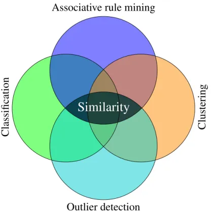
• Classification: Partitioning the data to a known structure. For example, a character written on the touch screen of a mobile phone is compared to the stored templates and decided which character it is.

• Clustering: Discovery of groups of data that are similar to each other. For example, clusters can be identified in sales history data which can lead to refined product placement.

• Outlier detection: Identification of uncommon data that can be interesting for further investigation. For example, unusual heartbeats in ECG data can be identified.

• Associative rule mining:Detecting internal relationships inside the dataset. For example, it can be determined that a specific behavior of a variable forecasts faulty end product during production.

These tasks share a common requirement: a (dis)similarity measure has to be defined between the elements of a given database. Moreover, from simple clustering and classification to complex decision-making systems, the results of a data mining application are highly dependent on the applied (dis)similarity measure, as it is illustrated in Figure 1.1.

As it can be seen, the selected similarity measure has a key role in data mining.

Utilizing the flexibility provided by the elastic similarity measures (see Section 2.4) and overcoming their run-time issues [20, 18], it seems there is no more place for development in this area. Yet, this is far from reality.

Associative rule mining

Outlier detection

Clustering

Classification

Similarity

Figure 1.1. Common tasks in data mining and their relation to similarity The main advantage provided by the current elastic similarity measures used for time series data mining is that they are capable of relaxing the temporal axis.

Can this property always be enough? I showed in my M.Sc. thesis [21] that the answer is No. It was empirically proven that the current (dis)similarity measures that were developed with static univariate time series in mind are not adequate for other common sequences like multivariate time series with complex correlation structure or for time series of dynamic processes.

Facing these limitations and building upon the experiences with the most popular dissimilarity measures during my daily development engineering work motivated me to reconsider the current elastic measures. This led to the introduction of two novel dissimilarity measures and a new way of avoiding pathological warnings in case of dynamic time warping. Moreover, the result of this reconsideration is not only this thesis but the improved performance of the state of the art and market leading ultrasonic-based blind spot monitoring system [22].

The work described by this thesis is presented in the following structure:

Chapter 2 – Background gives a short overview on the basics of time series data mining. Time series representations and segmentation problems are discussed first and then the most popular elastic dissimilarity measure — dynamic time warping

— is reviewed in detail.

Chapter 3 – Correlation-based dynamic time warping discusses the first novel dissimilarity measure I defined for multivariate time series by combining principal component analysis-based segmentation and dynamic time warping. I proved that the presented algorithm provides better results than the currently used dissimilarity measures in case of multivariate time series with complex correlation structure.

Chapter 4 – Process dynamics-aware segmentationintroduces a new segmen- tation method, which enables the segmentation of multivariate time series according to the changes in process dynamics. This way, the modified version of the algorithm presented in the previous chapter can compare and data mine multivariate time series based on process dynamics.

Chapter 5 – Automatic constraining of dynamic time warping shows how correlation-based dynamic time warping inspired another novel similarity measure for time series segmented using piecewise linear approximation. The presented simi- larity measure can be combined with the classical, mean-based similarity measure to achieve more accurate results than that of the existing methods. Moreover, using this combined similarity measure, I empirically proved that similarity measures considering multiple features shorten the warping path and thus they reduce the possibility of pathological warpings and enable omission of global constraints.

Chapters 6 and7 – SummaryandÖsszegzéssummarize the three theses pre- sented throughout chapters 3 to 5 both in English and in Hungarian.

Chapter 8 – Publications related to the thesislists all the publications of the author that connected to the thesis.

Chapter 2

Background

2.1 Basic definitions and notation

Let us say, thatXndenotes ann-variable,m-elementtime series, wherexi is thei^th variable andx_i(j)denotes itsj^th element:

X_n= [x₁, x₂, x₃, . . . , x_n],

x_i = [x_i(1), x_i(2), . . . , x_i(j), . . . , x_i(m)]^T

(2.1)

According to this notation, a multivariate time series can be represented by a matrix in which each column corresponds to a variable and each row represents a sample of the multivariate time series at a given time:

h x₁ x₂ . . . x_n ⁱ



















X_n(1) X_n(2)

... X_n(m)





































x₁(1) x₂(1) . . . x_n(1) x₁(2) x₂(2) . . . x_n(2)

... ... ... ... x₁(m) x₂(m) . . . x_n(m)



















(2.2)

ThedissimilaritybetweenX_nandY_nrepresents how stronglyX_nandY_nresem- ble each other and assigns a non-negative real number to show this relation:

d(X_n, Y_n) :T xT →R⁺0, (2.3) where T denotes the domain of the time series withd(X_n, Y_n) = d(Y_n, X_n),

0≤d(X_n, Y_n)andd(X_n, X_n) = 0.

Similarityof time series can also be defined for arbitrarily selected finite value of k:

s(X_n, Y_n) :T xT →R^k0, (2.4) wherek 6= +∞,s(X_n, Y_n) =s(Y_n, X_n),0≤ s(X_n, Y_n)≤k ands(X_n, X_n) = k. In such cases, the dissimilarity of two multivariate time series can be derived from similarity:

d(X_n, Y_n) =k−s(X_n, Y_n) (2.5) A dissimilarity measure is considered adistance(metric) if it satisfies the trian- gular inequality, i.e.:

d(X_n, Y_n) +d(Y_n, Z_n)≥d(X_n, Z_n) (2.6)

2.2 Time series representations

Therepresentation of time seriesX_n is an arbitrarily selected feature set that de- scribes the original data:

r(X_n) :T → F, (2.7) whereF is the range of the selected feature set.

The most obvious time series representation is the unmodified, raw data:

r(X_n) = X_n (2.8)

The raw data, however, cannot often be used directly and the reason for this is not only the fact that usually some kind of data preprocessing is necessary to remove noise, unify different sampling rates, prepare time series for the selected (dis)similarity measure, etc. These preprocessing steps are usually done before any representation is applied.

A representation is selected for two main reasons. First, to provide a more suitable description of the original data and second, to compact the time series and thus to speed up the calculation of (dis)similarity measures this way. Selecting the proper representation of the time series for a given task has then always been a

t

Amplitude

ECG signal PAA representation

(a) PAA representation

t

Amplitude

ECG signal PLA representation

(b) PLA representation

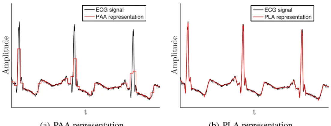
Figure 2.1. 50segment long PAA (piecewise aggregate approximation) and PLA (piecewise linear approximation) representations of an ECG signal originally con- taining2000samples

crucial factor in every application dealing with time series data. The representation does not only determine how accurately the original time series will be approximated, but it also narrows down the choice of (dis)similarity measures and thus affects the end result itself.

As of 2015, an actual^∗ example is indirect tire pressure monitoring (TPMS).

Here, no pressure sensors are built into the tires, but the time series provided by the wheel speed sensors are used to determine the tire pressure. With the help of the fast Fourier transform, the time series of the wheel speed sensors are represented in frequency domain instead of time domain. With this approach, it is possible to monitor the resonance frequency of a tire, which is correlated with the tire pressure [23].

Another example is shown on how important the selection of the representation is in Figure 2.1. An electrocardiograph (ECG) signal, containing2000data points, was approximated by piecewise aggregate approximation (PAA) and piecewise linear approximation (PLA) using50segments in both cases. It is easy to see that while PLA is capable of resembling the ECG signal, PAA would be suboptimal choice with this segment number.

Motivated by the need of finding the representation suiting the original time series the best for a given task, a large number of time series representations — alongside the matching dissimilarity measures — have been introduced by the time series data mining community: episode segmentation [24], discrete Fourier

∗From November 1, 2014, all new passenger cars sold in the European Union must be equipped with tire pressure monitoring system.

Time Series Representations

Data Adaptive

Symbolic

Natural

Language Strings

Symbolic Aggregate Approximation

Clipped Data

Trees Piecewise Polynomials

Piecewise Linear Approximation

Singular Value Decomposition

Adaptive Piecewise

Constant Approximation

Non-Data Adaptive

Piecewise Aggregate Approximation

Spectral

Discrete Fourier Transform

Discrete Cosine Transform

Chebyshev Polynomials

Random

Mappings Wavelets

Model-based

Hidden Markov Models

Statistical Models

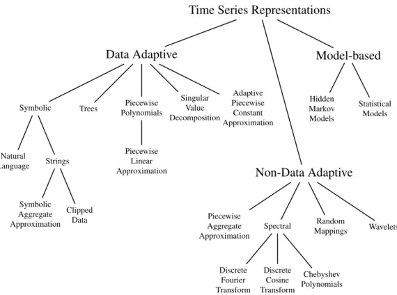
Figure 2.2. Hierarchy of basic time series representations according to Wanget al.

[33] extended with model-based approaches

transform (DFT) and discrete wavelet transform (DWT) based approaches [25, 26], Chebyshev polynomials [27], symbolic aggregate approximation (SAX) [28], perceptually important points [29], derivative time series segment approximation [30], implicit polynomial curve-based approximation [31], principal component- based approximation [32], etc. All proposed to compete and replace classical time series representations such as the above shown PAA and PLA, methods that has been used — and still preferred — in several engineering application thanks to their intuitiveness and ease of visualization. Data acquisition systems also echoed this trend, and in most systems different approximations of the raw data can be selected allowing to choose the one which suits the performed task the most.

Categorization of these representations can be made considering different prop- erties. For example, Lin et al. [28] and Wang et al. [33] determined two basic categories, data adaptive and non-data adaptive representations that can be extended with model-based approaches as it is shown in Figure 2.2. Similarly, representations can also be categorized whether they represent the data in the same domain (PAA, PLA, etc.) or project them to a new one (DFT), etc.

In the next four subsections, a short overview of the representations used through-

out the creation of this thesis is given.

2.2.1 Piecewise aggregate approximation

The most simple and intuitive time series representation method is piecewise aggre- gate approximation (PAA), which was proposed for the data mining community by two authors independently [34, 35]. To reduce the data fromn toN dimensions, where(N < n), time series are simply divided intoN equal sized sections and the average value of each segment is calculated. Assuming thatN is a factor ofn:

P AA(x) =x x(i) = N

n

n Ni

X

j=_Nⁿ(i−1)+1

x(j), (2.9)

wherexis a time series andx(i)is the mean value of itsi^th PAA segment. As PAA assigns the mean value to each segment, basically any dissimilarity measure can be used to calculate the dissimilarity between two PAA segments. For example, the Euclidean distance,d_ED, betweenx(i)andy(i)can be defined as follows:

d_ED =^q(x(i)−y(j))², (2.10) Besides the noise filtering resulted form averaging, PAA can compensate phase shifts of the temporal axis and different sampling rates of time series, but it cannot handle “locally elastic” shifts of time axis, and it is not an optimal choice for time series that should be described by the changes in its slope (see Figure 2.1(a)). In such cases, piecewise linear approximation (PLA) is a better option.

2.2.2 Piecewise linear approximation

Piecewise linear approximation (PLA) replaces the original data with not equally sized segments of straight lines, i.e. a PLA segment of time seriesxis described by four numbers:

P LA(x) = x

x(i) = [l_i, r_i, x(l_i), x(r_i)],

(2.11)

wherel_i andr_i are the first and last (left and right) time coordinates of thei^th PLA segment of x, x(l_i)and x(r_i)are the values of xin thel_i^th and ther_i^th time coordinates.

As it is shown in Figure 2.1(b), PLA usually provides a tighter representation than PAA as the length of a segment is not fixed. The closer approximation, however, also means that the selection of the dissimilarity measure is more complicated.

Vullings [36], after suggesting usage of slope of the segments [37], introduced several dissimilarity measures for ECG signal comparison based on the slope, run and rise of the PLA segments.

In the same time, Keogh and Pazzani [38] gave a generalized dissimilarity measure between two PLA segmentsx(i)andx(j)for dynamic time warping (DTW, see Section 2.4) by comparing the averages of the PLA segments:

d_{M P LA}(x(i), x(j)) = x(l_i) +x(r_i)

2 −x(l_j) +x(r_j) 2

!2

(2.12)

2.2.3 Symbolic aggregate approximation

Although PLA usually provides tighter representation than PAA, PAA has a very important advantage: it can easily be applied to streaming (on-line) data as the length of the segments is fixed and it does not necessarily depend on the data itself.

Arisen from PAA, Lin et al. [28] presented a new symbolic representation, called symbolic aggregate approximation (SAX), which combined the advantages of the data mining-driven representations with the symbolic representations popular in bioinformatics [39]. Such combination enabled the usage of awealth of data structures and algorithms from the text processing and bioinformatics communities [28]. Moreover, it made possible to define dissimilarity measures between the SAX- represented and between the original time series in a way that the former one always lower bounds the latter one, i. e. indexing becomes possible (see Section 2.4.3 on indexing).

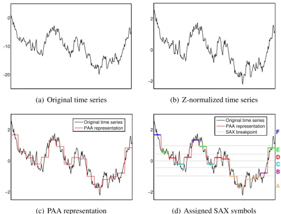
SAX representation of time seriesxcan be achieved with the following three steps:

1. Z-normalization:Ensure thatxhas0mean and standard deviation of1.

2. Segmentation:Create PAA representation ofx.

3. Symbol assignment: Assign symbols ’A’, B’, ’C’, etc. to PAA segments

−20

−10 0

E

(a) Original time series

−2 0 2

E

(b) Z-normalized time series

−2 0 2

Original time series PAA representation

E

(c) PAA representation

−2 0 2

Original time series PAA representation

SAX breakpoint F

A B C D E

(d) Assigned SAX symbols

Figure 2.3. Creating SAX representation of a time series shown in figure (a): z- normalization (b), PAA representation (c) and symbol assignment (d)

ensuring that the determined breakpointsβ₀. . . β_m that are used for symbol assignments produce each symbol with equal probability.

To ensure the equal probability of the symbols, Lin et al. [28] defined the breakpoints that theyare a sorted list of numbers[. . . ] such that the area under a [. . . ] Gaussian curve fromβ_itoβ_i+ 1= 1/m (β₀ andβ_mare defined as−∞and∞ respectively. Figure 2.3 shows the steps of creating SAX representation of a time series.

2.2.4 Principal component analysis

In the previous three subsections, representation methods created originally for univariate time series have been presented. Although such representations can be extended to multivariate time series, a multivariate time series is not only a set of univariate time series considered in the same time horizon. Instead, the correlation between the variables often characterizes them better than the actual values of the variables. This correlation can be treated as a hidden (latent) process and it is desirable to compare the time series based on it.

Figure 2.4. Dimension reduction with the help of PCA from 3 (filled dots) to 2 (textured dots) dimensions. Note how the correlation between the dots is preserved.

One of the most frequently applied tools to discover such a hidden process is principal component analysis (PCA) [40]. The main advantages of PCA are its optimal variable reduction property [41] and its capability to put the focus on the latent variables. Such properties made it ideal for industrial applications deal with a large number of variables [42].

The aim of PCA is to find the orthonormaln×nprojection matrixP_nthat fulfills the following equations:

Y_n^T =P_n^TX_n^T, P_n⁻¹ =P_n^T

(2.13)

whereX_nis the multivariate time series with lengthmandY_nis the transformed data having diagonal covariance matrix. The raws of P_n are the new base for representingXnand they are called principal components.

To solve Equation 2.13, PCA linearly transforms the original, n-dimensional data to a new, p < n-dimensional coordinate system with minimal loss of infor- mation in the least square sense. It calculates the eigenvectors and eigenvalues of the covariance (or correlation) matrix of then-dimensional data, and selects the largestpeigenvalues (λ₁, . . . , λ_p) with the corresponding eigenvectors as a new basis.

Technically speaking, PCA finds the most significantporthogonal directions with the largest variance in the original dataset as it is shown in Figure 2.4.

Measures of PCA models

One of the reasons PCA is used is its variable reduction property, i.e. when only the firstp < nprincipal components are used for the projection. To measure the accuracy of the PCA model, the percentage of the captured variance can be used:

Pp i=1λi

Pn

i=1λ_i, (2.14)

whereλ₁, . . . , λ_nare the eigenvalues of the covariance matrix ofX_n. Knowing how much percentage of the variance is wished to be explained by the PCA model, the number of retained principal components can be determined.

Another popular method to select the appropriate number of components is to visualize the eigenvalue against the component number, i.e. the scree plot. Usually, the first few principal components describe the major part of the variance while the remaining eigenvalues are relatively small. Looking for an “elbow” on the scree plot, the number of principal components can also be determined.

When the PCA model has adequate number of dimensions, it can be assumed that the distance of the data from thep-dimensional space of the PCA model is resulted by measurement failures, disturbances and negligible information. Hence, it is useful to analyze the reconstruction error of the projection. It can be computed for thej^th data point of the time seriesX_nas follows:

Q(j) = (X_n(j)−X_n(j))(X_n(j)−X_n(j))^T

=X_n(j)(I −U_Xn,pU_X^T

n,p)X_n(j)^T,

(2.15)

whereX_n(j)is thej^thpredicted value ofX_n,Iis the identity matrix andU_pis the matrix of eigenvectors. These eigenvectors belong to the most importantp≤n eigenvalues of the covariance matrix ofX_n, i.e. they are the principal components.

The analysis of the distribution of the projected data is also informative. The Hotelling’s T² statistic is often used to calculate the distance of the mapped data from the center of the linear subspace. Its formula is the following for thej^th point:

T²(j) = Y_p(j)Y_p(j)^T, (2.16) whereY_p(j)is the lower (p) dimensional representation ofX_n(j).

Figure 2.5 shows theQand theT²measures in case of a2-variable11-element time series. The original time series data points are represented by grey ellipses and

X2

T² Q

X1

Figure 2.5. Measures of PCA-models: Hotelling’sT²statistics and theQreconstruc- tion error

the black spot marks the intersection of the axes of the principal components, i.e. the center of the space that was defined by these principal components.

PCA-based similarity measures

Krzanowski [43] defined a similarity measure, called PCA similarity factor, by comparing the principal components (the dimensionality reduced, new coordinate systems) as follows:

s_{P CA}(X_n, Y_n) = trace(U_X^T_n,pU_Yn,pU_Y^T_n,pU_Xn,p)

p , (2.17)

whereX_nandY_nare the two multivariate time series withnvariables,U_Xn,pand U_Yn,pindicate the matrices of eigenvectors that belong to the most importantp≤n eigenvalues of the covariance matrices ofXnandYn, i.e. the two new bases of the projections ofX_nandY_n.

The PCA similarity factor has a geometrical explanation, because it measures the similarity between the two new bases by computing the squared cosine values between all the combinations of the first pprincipal components fromU_Xn,p and U_Yn,p:

s_{P CA}(X_n, Y_n) = 1 p

p

X

i=1 p

X

j=1

cos²Θ_i,j, (2.18)

whereΘ_i,j is the angle between thei^th principal component ofX_nand thej^th principal component ofY_n.

Although the PCA similarity factor made it possible to compare time series based on the latent variables, i.e. the “rotation” of the principal components, it weights all principal components equally while the principal components do not describe the variance equally. Johannesmeyer [44] modified the PCA similarity factor and weighted each principal component according to the variance it explains, i.e. its eigenvalue:

s^λ_{P CA}(X_n, Y_n) =

Pp i=1

Pp

j=1(λ^X_i ⁿλ^Y_jⁿ) cos²Θ_i,j

Pp

i=1λ^X_i ⁿλ^Y_iⁿ , (2.19) whereλ^X_i ⁿ andλ^Y_jⁿ are the corresponding eigenvalues for thei^th andj^thprincipal component ofX_nandY_n.

Yang and Shahabi [45] moved one step forward and presented an extension of the PCA similarity factor, called Eros (Extended Frobeniusnorm). Eros compares the principal components with the same importance and instead of using their eigenvalues as weight, which is learned from a learning set. For twon-variable time seriesXn, Y_nand for the corresponding matricesU_Xn andU_YnEros is defined as:

s_Eros(X_n, Y_n) =

n

X

i=1

w_i|U_Xn(i)U_Yn(i)^T|=

n

X

i=1

w_i|cos Θ_i|, (2.20) wherecos Θ_i is the angle between the two corresponding principal components andw_iis theielement of the weighting vector that is based on the eigenvalues of the sequences in the learning set.

Although Eros proved its superiority over the standard PCA similarity factor, and even an indexing structure was introduced for it [46], Eros still carries the burden of all PCA-based similarity measures: none of the presented methods can consider the alteration of the correlation structure and thus cannot handle the fluctuation of the latent variables. Correlation-based dynamic time warping (CBDTW) is presented in Section 3.1 to address this drawback of all PCA-based similarity measures by utilizing dynamic time warping and correlation-based segmentation.

2.3 Segmentation problem

To provide a compact, comparable representation of time series, segmentation is often applied, where a number (or a set of numbers) represents each segment according to the selected representation method.

By definition, thei^thsegment of multivariate time seriesX_nis a set of consecutive time points:

S_i(a, b) = [X_n(a);X_n(a+ 1);. . .;X_n(b)], (2.21) wherea < b. Thec-segmentation ofX_nis a partition ofX_ntocnon-overlapping segments:

S_X^c_n = [S1(1, a);S2(a+ 1, b);. . .;Sc(k, m)] (2.22) In other words, a c-segmentation splits X_n to cdisjoint time intervals, where 1≤aandk ≤m.

The segmentation problem can be framed in several ways [19], but its main goal is always the same: find homogeneous segments by the definition of a cost function,cost(S_i(a, b)). This function can be any arbitrary function which projects the space of time series to the space of the non-negative real numbers. Usually, cost(S_i(a, b))is based on the differences between the values of thei^thsegment and its approximation by a simple functionf (constant or linear function, a polynomial of a higher but limited degree):

cost(Si(a, b)) = 1 b−a+ 1

b

X

l=a

d(Xn(l), f(Xn(l))) (2.23) Thus, the segmentation algorithms simultaneously determine the parameters of the models and the boundaries of the segments by minimizing the sum of the costs of the individual segments:

cost(S_X^c

n) =

c

X

i=1

cost(S_i(a, b)) (2.24) This segmentation cost can usually be minimized by dynamic programming, which is computationally intractable for many real datasets [47]. Consequently, heuristic optimization techniques such as greedy top-down or bottom-up techniques are frequently used to find good but suboptimalc-segmentations.

• Bottom-Up: Every element ofX_nis handled as a segment. The costs of the adjacent segments are calculated and two segments with the minimum cost are merged. The merging cost calculation of adjacent segments and the merging are continued until some goal is reached.

split are calculated and the one with the minimum cost is executed. The splitting cost calculation and splitting is continued recursively until some goal is reached.

• Sliding Window: The first segment is started with the first element ofX_n. This segment is grown until its cost exceeds a predefined value. The next segment is started at the next element. The process is repeated until the entire time series is segmented.

All of these segmentation methods have their own specific advantages and draw- backs. Accordingly, the sliding window method is the fastest one and can be applied for streaming data; however, it is not able to divide up a sequence into a predefined number of segments. The applied method depends on the given task. Keoghet al.

[48] examined these heuristic optimization techniques through the application of piecewise linear approximation in detail and concluded that if real-time (on-line) seg- mentation is not required, the best result can be reached via bottom-up segmentation.

Its pseudocode is shown by Algorithm 2.1.

Algorithm 2.1:Pseudocode of the generic bottom-up segmentation algorithm Input: X_n: sequence to be segmented

Input: total_cost: target total cost, e.g. summarized representation error in case of PLA segmentation

Data: S: structure that represents the segmented sequence

Data: merge_cost: structure that contains the merge costs of adjacent segments

Output: S^c_Xn: c-segmentation ofX_n

/* Consider every data point as a segment at initialization */

for(i = 1; i <= length(X_n); i++)do S(i) = X_n(i);

end

/* Calculate the cost of adjacent segments */

for(i = 1; i < length(X_n); i++)do

merge_cost(i) = cost(concatenate(Xn(i) ,Xn(i+1)));

end

/* Continue merging until some goal, e.g. number of segments or total cost, is reached */

while(length(S) < wished_number_of_segments)

|| (sum(merge_cost)) < total_cost)do /* Find lowest cost to merge */

lowest = min(merge_cost));

/* Concatenate the two adjacent segments for which the lowest cost is belong to */

S(lowest) = concatenate(S(lowest), S(lowest+1));

/* Update the structure of segmented sequence */

delete(S(lowest+1));

/* Update merge_cost */

merge_cost(lowest) = cost(concatenate(S(lowest),S(lowest+1)));

merge_cost(lowest-1) = cost(concatenate(S(lowest-1),S(lowest)));

delete(merge_cost(lowest+1));

end

/* Provide c-segmentation results */

S^c_Xn =S;

2.4 Dynamic time warping

The increasing and less costly computational power made it possible to consider similarity measures with more computational demand for tasks where the quality of the comparison is much more important than the speed of the calculation. Non-linear matching techniques that are capable of considering local time shifting, have been studied extensively for this purpose including longest common subsequences (LCSS) [49], edit distance on real sequences (EDR) [50], edit distance with real penalty [51], sequence weighted alignment [52], spatial assembling distance [53], etc.

Dynamic time warping (DTW), which has long been known in the speech recog- nition community [54], excelled these methods in popularity thanks to its adaptability [55], efficiency [33] and extensive literature [17]. Since its first appearance, dynamic time warping has been successfully applied for a large variety of problems in several different disciplines, such as gene alignment [3], gait detection [6], fingerprint recog- nition [7], signature verification [8, 14], weather prediction [9], song recognition based on humming [56] and even for sewer flow monitoring [16].

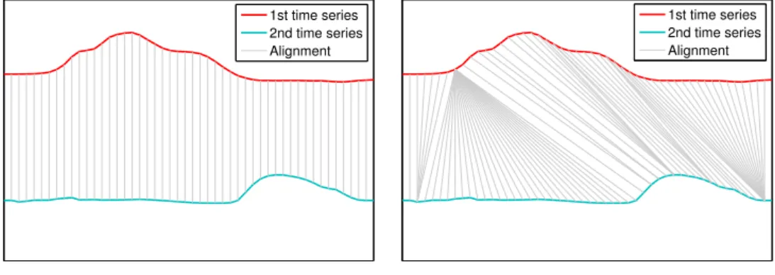
DTW is not a simple similarity measure, rather a framework. DTW allows the selection of the local dissimilarity measure that is used to compare the elements of the time series, also it “warps” the temporal axis and thus enables to compare the similar features to each other. To demonstrate such warping capability, an example is shown in Figure 2.6. Two time series are compared with the rigid Euclidean distance and with DTW, which in this case also utilized Euclidean distance as the local distance. The compared data points are connected by grey lines and it is easy to see that the flexibility provided by DTW resulted in more natural alignments.

1st time series 2nd time series Alignment

(a) Alignments with Euclidean distance

1st time series 2nd time series Alignment

(b) Alignments created by DTW

Figure 2.6. Alignments (gray lines) generated by Euclidean distance and dynamic time warping

2.4.1 Formal definition of dynamic time warping

Letxandydenote two univariate time series with lengths ofnandmand with time indexest_xand t_y, i.e. x(t_x(j)) = x(j). A non-warping dissimilarity measure can then, for example, be defined as follows:

d(x, y) =

n=m

X

j=1

d(x(j), y(j)), for allj ∈t_x(j) =t_y(j) (2.25) Putting it in other words, a non-warping dissimilarity measure requires that the compared time series be the same in length and have the same time indexes. In many cases, however, such conditions cannot be fulfilled or it is not wished as some kind of flexibility is expected when the time indexes are compared. To provide this flexibility, a more general dissimilarity measure can be introduced that allows alignment of time indexes [17]:

d_φ(x, y) =

k

X

j=1

d(φ_x(j), φ_y(j))/K_φ, (2.26) whereK_φis a normalization constant,φ_x andφ_y are monotonically nondecreas- ing time warping functions that maintain the temporal order of the original time indexes:

t_x =φ_x(j), j = 1, . . . , k t_y =φ_y(j), j = 1, . . . , k

(2.27)

Theφ_x, φ_y function pair creates a common time axis, called warping path. The question is, however, which warping path should be selected from the large number of the possible candidates. A popular and desirable choice is to define dynamic time warping dissimilarity as the minimum of all possible warpings:

d_{DT W}(x, y) = arg min

φx,φy

d_φ(x, y) (2.28)

2.4.2 Calculation of dynamic time warping

In order to calculate d_{DT W} of Equation 2.28, a grid D with size n ×m can be defined in which each cell represents the dissimilarity between the corresponding data points of the two time series (see Figure 2.7). As it was mentioned previously, any application-dependent dissimilarity measure likeL norms including Euclidean

1 2 3 4 5 6 7 8 9 10 11 12 1

2 3 4 5 6 7 8 9

Figure 2.7. Grid Dand the optimal warping path of DTW of the two time series shown below and on the left of the grid

distance can be used to calculate the dissimilarity between the time series data points.

Considering the Euclidean distance one can have:

D(i, j) = ^q(x(i)−y(j))² (2.29) Using gridD, many arbitrary mappings — the warping paths — betweenxand ycan be created. However, the construction of a warping pathpis restricted by the following constraints:

• Boundary condition: The path has to start in D(1,1) and end in D(n, m), wherenandmare the length of the two time series to be compared.

• Monotonicity:The path has to be monotonous, i.e always heading fromD(1,1) toD(n, m). Ifp(k) = D(i, j)andp(k+ 1) = D(i⁰, j⁰)theni⁰ −i ≥ 0and j⁰−j ≥0.

• Continuity:The path has to be continuous. Ifp(k) =D(i, j)andp(k+ 1) = D(i⁰, j⁰)theni⁰−i≤1andj⁰−j ≤1.