Graph Coloring based Heuristic for Crew Rostering
L´ aszl´ o Hajdu
a, Attila T´ oth
b, and Mikl´ os Kr´ esz
cAbstract
In the last years personnel cost became a huge factor in the financial management of many companies and institutions.The firms are obligated to employ their workers in accordance with the law prescribing labour rules.
The companies can save costs with minimizing the differences between the real and the expected worktimes. Crew rostering is assigning the workers to the previously determined shifts, which has been widely studied in the literature. In this paper, a mathematical model of the problem is presented and a two-phase graph coloring method for the crew rostering problem is introduced. Our method has been tested on artificially generated and real life input data. The results of the new algorithm have been compared to the solutions of the integer programming model for moderate-sized problems instances.
Keywords: crew rostering, graph coloring, tabu search
1 Introduction
In certain areas of the industry, the workers’ work is performed not in a fixed order.
The work activities are organized into shifts, which may vary in duration, time of the day and other properties. In generally, every worker has a contract with a defined expected worktime and a base salary for that, hence the overtime or the undertime is a large-scale extra cost for the company. In the life of the companies, the human cost is a significant part of the complete budget, hence they want to employ the workers in the most efficient way. In most cases, the scheduling of the workers has two different steps (see Figure 1.). The first is the crew scheduling which means that the daily tasks are catenated into shifts so that each shift must meet the law constraints. The second step is the crew rostering. In this step the question is that how to assign the crew members to shifts for a work period called planning period which is typically being 1-3 month long. This study concentrates
aUniversity of Szeged, InnoRenew CoE and University of Primorska. E-mail:
hajdul@inf.u-szeged.hu, ORCID:https://orcid.org/0000-0002-1832-6944.
bUniversity of Szeged, Hungary. E-mail: attila@jgypk.u-szeged.hu, ORCID:
https://orcid.org/0000-0003-1014-7965.
cUniversity of Szeged, InnoRenew CoE and University of Primorska. E-mail:
kresz@jgypk.u-szeged.hu, ORCID:https://orcid.org/0000-0002-7547-1128.
DOI: 10.14232/actacyb.281106
on the rostering phase. It is important to note, that our solution is a proof of concept, even though it is possible to extend the core of the method with more complicated regulations. The objective of this paper is to show the efficiency of the core algorithm with basic regulations which are mostly used internationally as we did not intend to give a country specific solution. In real life applications very specific regulations are applied in several cases, such as the constraint of the travel time from home, or fair distribution of popular and not popular shifts can be also taken into account[2]. In summary, in real life environment the solution for crew rostering must meet some European Union and local regulations as well as the preferences of the workers.
Figure 1: Scheduling of workers
There are two different cases concerned in the workers-shifts assignment. In the first case the companies assign an optimal number of crew members to the pre- defined daily shifts minimizing the total cost. In the second case there is a given set of workers and the firm assigns the shifts to them in a most efficient way. In this paper we deal with the first case i.e. we have shifts and the main goal is to minimize the overall cost.
The crew rostering problem is based on the generalized set covering model.
Dantzig was the first who dealt with its mathematical application [7]. The crew rostering problem is NP-hard therefore it is generally considered that exact solution is not realistic to produce in the case of real life size problems. [12, 21, 18, 20, 25]
By the above reason as a consensus of theory and practice, heuristic algorithms are used. The crew rostering solution methods have a quite rich literature, several overviews are available [4, 9, 22, 24, 10, 27]. The literature provides numerous examples of the issue, among which the most significant ones are the airline crew rostering [15], railway crew scheduling [17] and the driver scheduling [1, 19]. In the literature, the studies are generally grouped around the related application areas. These solutions need to correspond to the regulations of the company as well as to the ”national norms”. In most cases the regulations are different in each area, for instance the qualifications of the workers are handled in different ways in airline crew rostering, while in driver rostering it is usually ignored. These regulations are formalized as constraints which usually have two different types. A hard constraint must not be violated, while in a case of a soft constraint it is allowed with being penalized by some extra cost. For example single workday in a long days- off period or work in a requested days-off can be handled by soft constraints. In this paper, we only deal with hard constraints but the model and methodology can be easily extended to soft constraints with using appropriate penalties in the objective function.
Taking into consideration the basic regulations of all the significant areas (typ- ically regulated in national laws) we have applied the following constraints:
1. A worker can have maximum one shift in one day.
2. There is a minimum rest time between two shifts.
3. There is a maximum total worktime during one week.
4. There is a minimum number of days-off in one month.
5. There is a maximum number of consecutive workdays.
Every worker has a contract which determines the expected worktime. The difference between this defined worktime and the length of the shifts may produce overtime or undertime. For overtime the worker receives extra payment above the basic salary. However, the basic salary must be paid even in the case of undertime.
Therefore the human resource extra cost on the schedules shifts can be optimised through minimizing the overtime.
In this paper, we give a new heuristic solution method based on graph coloring which fits to many application area. Our algorithm has two main steps. In the initial rostering, the algorithm estimates the number of workers, builds a conflict graph from the shifts, and generates days-off pattern for every worker. One of the key innovations of the method is to generate days-off patterns which meet the basic regulations and create a frame for the problem, and to get the additional free days indirectly from the tabu search method. Afterwards the graph is colored, so an initial rostering is created by a modified greedy algorithm. When an initial solution is generated the graph is iteratively recolored with a tabu search method to reduce the cost. An important part of the method is to balance the shifts among workers to create a solution where workers are close enough to their expected workload.
The results of the algorithm have been compared to the results of the integer programming model with moderate problem size. These results show that our algorithm is efficient and robust. Our solution is a wireframe for the general crew rostering problem, however we tested our method in a real-life application area of the driver rostering case. In the next two sections the crew rostering problem is defined and the mathematical model of the problem is introduced. Finally, in Section 4 and 5 our heuristic method and the test results will be presented.
2 Problem formulation
The crew rostering problem is formally defined as the following. LetC be the set of workers. The set of shifts denoted byS which needs to be carried out. A shift is composed of a series of daily tasks. A shift is defined by its date, starting and ending time in the day, duty time (i.e. the time between the starting and ending time), and the working time. The working time might differ from the duty time since a shift may contain idle periods when the worker does not work. The aim
is to assign the crew members to the shifts with minimal cost. Consequently, let f =S →C be an assignment where the shifts are covered by the workers where exactly one worker assigned to each shift.
Let ct(i) be the contract type of worker i. The type of the contract defines the prescribed worktime in average for a single workday. Let aw(ct) denote the expected daily working hours by contract type ct. Based on the contract it is possible to calculate the expected worktime in the planning period. For example in our case, every crew member has a contract which defines eight working hours per day. In our model, the type of the contract is a parameter, therefore it is possible to deal with different contract types also. The expected worktime can be defined in the following way:
expected worktime(i) =number of workdays∗aw(ct(i)) i∈C (1) The basic employment cost is based on workers’ expected worktime defined by their contract. So in optimal case every worker will work according to her/his expected worktime. However, in case of working over the expected worktime, em- ployers have to provide extra salary for this overtime. Therefore, the cost is the following:
cost=α∗overtime+β∗employment cost (2) where α and β are pre-defined weights. In a real problem these multipliers can adjust the different costs to the preferences of the company. Following the practice we suppose that the employment cost is proportional to the working hours prescribed by the contract type. Hence, the objective function will consider in the minimization both the overtime and the number of workers. We also assume that the planning period P is fixed (typically 1-3 months) and all the rules having no specified time period (e.g. the average working time) are considered with respect toP; with this approach we follow the practice as well.
3 Mathematical model
LetD be the set of the days, W eek the set of the weeks and M onthe set of the months in the given planning period. ConsequentlyDW eekw denotes the days of the weekw andDM onm is the days of the monthm. Meanwhile the length of the plan- ning period (the number of days) is defined byl, and letlm be the number of days in the monthm. The set of the workers is denoted byC, and the set of shifts byS whereSpis the set of shifts on dayp. LetSSjkis a compatibility relation between the shifts, where its value is 1 if shiftj and shift k can be assigned to the same worker, and 0 otherwise (can be used to define Rule 2). LetW T be the maximum worktime on a week (for Rule 3), W D be the maximum number of consecutive workdays (for Rule 5) andDW Dp be such number of the consecutive days beginning from day p (W D+ 1 days in a row). The minimum number of days-off is de- noted byRD(for Rule 4). Let the expected worktime in a month beaw(ct(i, m)),
wherem∈M onandi∈C . In order to minimize the number of workers letcc(i) be the operational cost of worker i, i.e the base salary. Let wt(j, p) be the work- time of shiftj on day p. Finally let αbe the weight of the overtime andβ be the weight of the employment cost. We need the following variables to define the model:
Driveriassigned to shiftj:
xij∈ {0,1} ∀i∈C, ∀j ∈S (3) Driveriworks on day p:
zip∈ {0,1} ∀i∈C, ∀p∈D (4) Driveriworks in the planning period:
yi∈ {0,1} ∀i∈C (5)
Overtime of workeri:
πi≥0 ∀i∈C (6)
The constraints of the integer programming model are the followings:
Exactly one worker is assigned to each shift.
X
i∈C
xij= 1 ∀j∈S (7)
There is at most one shift assigned to worker on a given day.
X
j∈Sp
xij =zip ∀i∈C, ∀p∈D (8)
An employee works in the planning period if he/she has at least one shift.
X
p∈D
zip≤lyi ∀i∈C (9)
The following constraint excludes the possibility of assigning two incompatible shifts to a worker.
xij+xik≤SSjk+ 1 ∀i∈C, ∀j, k∈S (10) The worktime must not exceed the maximum working time in any week.
X
p∈DW eekw
X
j∈Sp
xijwt(j, p)≤W T ∀i∈C, ∀w∈W eek (11)
A worker can have at most the maximum number of consecutive shifts.
X
p∈DW Dq
zip≤W D ∀i∈C, ∀q∈D (12)
At least the required number of days-off have to be given for each worker in a month.
X
p∈DM onm
zip≤lm−RD ∀i∈C, ∀m∈M on (13) Let us define the overtime.
X
m∈M on
( X
p∈DM onm
X
j∈Sp
xijwt(j, p)−aw(ct(i, m)))≤πi ∀i∈C (14)
The objective function minimizes the sum of the weighted overtime and the oper- ational cost.
minX
i∈C
(απi+βyicc(i)) (15)
The mathematical model is a good approach if the problem is relatively small because it gives an exact solution for the problem. Unfortunately in real life there are often too big problems for these solution methods therefore in most cases the companies use heuristics.
4 Heuristic method
Our algorithm is a two-phase graph coloring method (TPC), where in the first step an initial rostering is produced with a graph coloring procedure and in the second step this rostering is improved with the over- and undertime being minimized by tabu search. M. Gamache et. al [11] developed a method, where graph coloring algorithm based tabu search was used for scheduling pilots. These pilots have qual- ification and the objective is to find a feasible solution in a pre-specified workload interval. Nevertheless, in the literature tabu search method is a widely used tech- nique especially in bus driver scheduling or rostering. Some example papers using tabu search to solve the scheduling problem (defining the shifts) are [6, 26], but the method was also successfully applied for laboratory personnel scheduling problems [3]. However, in our case both the problem and the solution method are different by two reasons: the regulations are different and here days-off patterns are used. Fur- thermore, we will give a general solution method for the crew rostering, serving as a framework to be specialized to several fields. In our approach by its universality and flexibility, days-off patterns will be applied with ak-coloring algorithm.
The TPC has the following steps:
1. Initial rostering.
a Estimate the number of workers.
b Generate days-off patterns.
c Build a conflict graph.
d Color the graph.
2. Tabu Search to improve the solution.
The initial rostering determines the number of workers, the days-off patterns and the initially colored graph. First, the algorithm estimates the optimal number of workers and for each worker generates a days-off pattern. These patterns will define whether a worker can work on a day or not. In the last two steps of the initial phase the conflict graph is built and colored. In most cases the cost of the initial rostering can be improved, therefore in the second phase the method switches the shifts between the workers with a local search method in order to minimize the cost of the rostering.
It is important to note that in our heuristic the objective function is divided into two parts (see Formula 2). The algorithm tries to minimize the number of workers in the initial phase, while the recoloring step is to minimize the overtime. A feature of the heuristic that we get better solution if we also minimize the undertime: we will see below that it is an equivalent approach with respect to Formula 2 and it will provide a solution in which the workload will be balanced among the employees.
Nevertheless, the general cost function of the method is based on the overtime and undertime only. Since the employment cost is proportional to the working hours by contract (expected worktime), we will see that Formula (2) is equivalent to the weighted linear combination of overtime and undertime. Formally, the overtime and the undertime definition and the cost of the heuristic are the following.
overtime=X
i∈C
max (0, worktime(i)−expected worktime(i)) (16)
undertime=X
i∈C
abs(min (0, worktime(i)−expected worktime(i))) (17)
cost=α0∗overtime+β0∗undertime (18) In order to clarify the equivalence of Formulas (2) and (18), notice that the total worktime required by the shifts (the sum of the worktime of all the shifts) in the whole planning period is a constant. Therefore it is easy to see that in any solution the expected worktime is equal to (total worktime−overtime+undertime). By this we obtain for Formula (2):
cost=α∗overtime+β∗(total worktime−overtime+undertime) (19) Then (β∗total worktime) is a constant and provides the basic theoretical lower bound in the cost. Thereforeα0 =α−β andβ0 =β will make Formulas (2) and (18) equivalent from optimization point of view with (18) expressing the extra cost above the basic theoretical lower bound.
4.1 Initial rostering
4.1.1 Estimate the number of workers
At first, the initial set of workers (C∗) needs to be defined wherewith the shifts can be effectively covered. The number of these workers can be estimated for the planning period using the total worktime of the shifts and the contracts of the workers. In our case we concern ”uniform workers” meaning that they have the same type of contracts, i.e. their expected worktime is the same. Basically, we suppose that the planning period is one or a few months (typically 1-3 months).
This assumption is general in real life situations, but it can be easily relaxed to any length of the planning period. Therefore, the number of the crew members for a given contract typectis given by the following way:
|C∗|=round
total worktime aw(ct)∗number of workdays
Practically, an initial set of workers is given in such a way that the expected worktime is assigned to all of the workers determined by the contract type in every day of working. In this way, the estimated number will be the cardinality where the difference of the total worktime and the expected worktime for this set is minimal.
A trivial lower bound for the number of workers can also be given by the number of the shifts on the busiest days, since one crew member can have at most one shift a day. Furthermore, if the estimated number of workers is known, a theoretical lower bound (LBot) for the overtime can be given by the following way:
LBot = max (0,(total worktime− |C∗| ∗aw(ct)∗number of workdays)) It is clear that with a given set of workers LBot is correct since the overtime is minimal in this case if every worker has workload at least according to his/her contract.
4.1.2 Generate days-off patterns
In some areas, it may be necessary to pre-specify days for a worker in advance when he or she does not work (called days-off) in the planning period (called days- off pattern). Some example for the usage of days-off patterns can be found in the literature [23, 8]. It is a widely accepted and used methodology to generate a days-off for the workers in the crew rostering. The advantage of the days-off patterns is that the days-off requested previously by the workers can be taken into account, as well as the 4th (minimum number of days-off in one month) and 5th (maximum number of consecutive workdays) rules are fulfilled here, so we do not have to concern these in the latter phases.
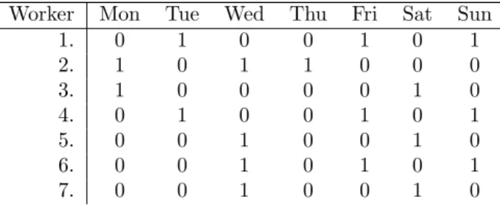
Days-off patterns define different fixed free days for each worker. We tried 3 different methods to generate the days-off patterns. At first we generated random patterns as presented in Table 1. The days-off are generated by weighted random generator which consider the number of the shifts on the days and Rule 4 and
Rule 5. On days with higher shift load the workers received a day off with lower probabilities than those days where lower number of shifts are. To formalize the probability let |C∗ | be the estimated number of workers and Sj denote the set of the shifts on the day j, the probability of the days-off on the day j is given by 1−(|Sj|/|C∗ |); if the generated days-off pattern doesn’t meet with the rules, we insert additional free days into the pattern randomly. The pattern vector is generated for every worker one by one.
Table 1: Random days-off patterns
Worker Mon Tue Wed Thu Fri Sat Sun
1. 0 1 0 0 1 0 1
2. 1 0 1 1 0 0 0
3. 1 0 0 0 0 1 0
4. 0 1 0 0 1 0 1
5. 0 0 1 0 0 1 0
6. 0 0 1 0 1 0 1
7. 0 0 1 0 0 1 0
The second tested pattern type was the so called 5-2 pattern (see Table 2).
Here, the workers get two days-off after each consecutive five workdays. These days-off patterns repeat a seven days long sub-pattern along the planning period such that if the sub-pattern starts at dayj* then from dayj* to dayj*+4 the days are workdays and daysj*+5 and j*+6 are days-off. The next pattern shifts the sub-pattern forward with one day. Therefore, seven different patterns are generated from this days-off pattern type.The 5-2 pattern seemed to be appropriate, since a week usually contains 5 workdays and 2 days off. Hence, if everyone will work by this 5-2 pattern, then their working hours are likely close to their expected worktime. It is clear that the 5-2 days-off patterns also meet the defined hard constraints.
We found that the random and the 5-2 patterns are too rigid and greedy with producing too much exclusion in the first phase. This means that during the graph coloring the days-off patterns exclude too many workers on days where they could possibly work.
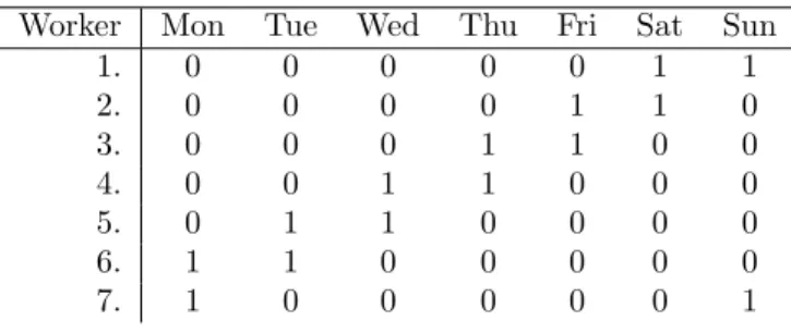
To overcome this problem the third pattern type defines minimal fixed days- off considering the rules. Thus, we propose a 6-1 days-off pattern which means that the workers get one fixed days-off after every six consecutive workdays. These patterns are generated with the same method as 5-2 patterns, but in the sub- pattern from daysj* toj*+5 are workdays and dayj*+6 is days-off (see in Table 3). This pattern meets both the minimal free days rule (Rule 4) and the maximal consecutive workdays (Rule 5) based on the European regulations (see in Section 5). It causes only a few exclusion during the graph coloring. Also, the tabu search will have a relatively big state space. Naturally, the pattern defines only fixed days- off and in the last phase we may get automatically some additional days-off in the
Table 2: 5-2 days-off patterns
Worker Mon Tue Wed Thu Fri Sat Sun
1. 0 0 0 0 0 1 1
2. 0 0 0 0 1 1 0
3. 0 0 0 1 1 0 0
4. 0 0 1 1 0 0 0
5. 0 1 1 0 0 0 0
6. 1 1 0 0 0 0 0
7. 1 0 0 0 0 0 1
final solution: when the workers are not assigned to a shift they automatically have a day off. Because of the days-off patterns, the 4th and 5th rules does not need to be taken into account later in step 2. In the Table 2 and Table 3 it is enough to give the day-off patterns for the first seven workers, since ifiandjare the indexes of the workers, and positive integers, furthermorei≡j mod(7) then thei−thand j−thworkers have the same days-off pattern.
Table 3: 6-1 days-off patterns
Worker Mon Tue Wed Thu Fri Sat Sun
1. 0 0 0 0 0 0 1
2. 0 0 0 0 0 1 0
3. 0 0 0 0 1 0 0
4. 0 0 0 1 0 0 0
5. 0 0 1 0 0 0 0
6. 0 1 0 0 0 0 0
7. 0 0 0 0 0 0 1
4.1.3 Build a conflict graph
LetG= (V, E) be a graph so called conflict graph, where every shift in the planning period is a vertex of the graph. There is an edge between two vertices if the corresponding shifts must not be performed by the same worker. For example if the time between two shifts is less than defined by the 2nd rule or they are on the same day.
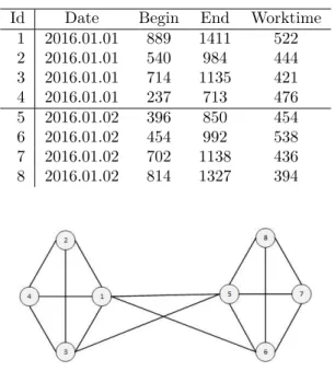
To understand the graph building let us see an example. Let the initial input of two days with 8 shifts is prescribed in Table 4. The shifts of each day compose cliques. There are 3 additional edges between them (1-5,1-6,3-5) because the time period between these shifts is less than the required one by Rule 2 (general value is 12 hours what we use here too). The generated graph is presented by Figure 2.
Table 4: Example shifts with their date,startin and ending time in minutes (0-1440 a day), and the contained working time in minutes.
Id Date Begin End Worktime
1 2016.01.01 889 1411 522
2 2016.01.01 540 984 444
3 2016.01.01 714 1135 421
4 2016.01.01 237 713 476
5 2016.01.02 396 850 454
6 2016.01.02 454 992 538
7 2016.01.02 702 1138 436 8 2016.01.02 814 1327 394
Figure 2: Example graph
4.1.4 Color the graph
Node coloring of a graph means assigning a color to each node in such a way that every neighboured node has different color. A coloring of the conflict graph gives a rostering for the problem if one color corresponds one worker. This rostering is correct since it fulfills the defined rules: Rule 1 and Rule 2 are guaranteed by the structure of the conflict graph, Rule 4 and 5 are fulfilled by the days-off pattern and Rule 3 is handled in the coloring. If we set the ending time of the vertices to the maximum of the increased value by the time of the 2nd rule and that of the end of the day, then we will obtain an interval graph. [16] There is efficient algorithm to color interval graph [14], but due to the extra restrictions of the crew rostering problem it becomes NP-hard. A good overview of the problem written by Kolen et. al [28]. Such a k-coloring algorithm is needed while adding a new color is possible. The initial estimation of the number of workers is usually correct, but some extraordinary inputs, e.g shifts with too short worktime, result such a graph that could not be colored with the estimated number of colors.Therefore we used the DSATUR algorithm which is effective and can be easily adopted to our needs (see Brelaz [5]) with coloring the nodes by their saturation values (saturation of a vertex represents the number of different color classes in its neighbourhood). Each
coloring iteration chooses the node with the highest saturation value and chooses the color where the corresponding worker is in maximum undertime. It starts with the estimated number of colors (i.e worker) and adds new color if it is necessary (i.e no available worker for a shift).
Algorithm 1Graph coloring.
1: While there is an uncolored vertex
2: Letv be the next uncolored vertex with the maximal saturation value
3: If there is an equal saturation we choose the vertex with maximal degree
4: C←available colors where the regulations are not violated
5: Choose available colorc∈C (i.e worker) with the lowest worktime.
6: Ifc does not exist letcbe a new color.
7: Assignc tov.
8: foreachvn∈neighbours of v do
9: vn ←update saturation value
10: end for
11: end while
The graph coloring gives an initial solution which meets the given constraints and assigns a worker to every shift. Since the real working time of each worker and their expected worktime is known, the initial cost can be calculated.
4.2 Tabu Search
The tabu search was introduced by Glover in 1986 and it is one of the most famous local search techniques [13]. The state space of the tabu search denoted by SL consists of all the feasible coloring patterns in the conflict graph. Each state is a coloring and the objective function has to be minimized onSL. The algorithm visits solutionssl0, sl1, ...sln∈L, where sl0 is the initial solution produced by the graph coloring and sli+1 ∈N(sli) with N(sl) denoting the set of neighbours ofsl. The next neighbour is chosen by a first fit method meaning that the first neighbouring solution is chosen being better than the actual solution and the neighbours are in a random order. Steps chosen in one step are stored in the tabu list denoted by T L. The steps in the list are forbidden to repeat. The neighbours of a solutionsl are defined by using the following operations:
1. Recoloring of a vertex: Another color is given to a vertex of the graph. It means that a shift is taken away from a worker and given to another one permitted by the constraints.
2. Swapping the colors of two vertices: The colors of two vertices are switched, therefore shifts are swapped between two workers in a way that both of them receive a shift which they can carry out with keeping the constraints.
The algorithm tries to change or swap a shift between the colors of the most undertimed worker and the most overtimed worker. After carrying out the vertex
recoloring or the vertex swapping, the step is added to the tabu list. So the moves are stored in the tabu list instead of the states. The elements spend a specified number of iterations in the tabu list, and if the length of the tabu list is greater than the max allowed iteration for an element on the list, then the oldest element which took the longest time on theT L, will be deleted from it. Pseudocode is given in Algorithm 2.
Algorithm 2Tabu search.
1: s0←initial solution
2: T L← ∅, s←s0, best←s0 3: while stopping criteriado
4: E←workers ordered by worktime
5: foreache1∈E f rom undertimed to overtimed orderdo
6: foreache2∈E f rom overtimed to undertimed orderdo
7: s∗ ←the f irst recoloring or swap between e1 and e2where cost(s∗)<
cost(s)and move(s, s∗)∈/ T L and goto line 10
8: end for
9: end for
10: if s∗not existthen
11: s∗ ∈N(s)the f irst solution where move(s, s∗)∈/ T L
12: end if
13: if cost(best)> cost(s∗)then
14: best←s∗
15: end if
16: T L←T L∪move(s, s∗)
17: if T L.size > max size of tabu listthen
18: Remove the oldest element from T L which took the longest time on the list
19: end if
20: s←s∗
21: end while
Multiple methods can be applied as stopping criteria. In most cases, the criteria is based on the iteration number or on the time bound. In our case, the algorithm stops if it can not find a better solution within a certain number of iteration.
5 Test results
In this section we will introduce the specific regulations for our case study, the test cases and the results of our algorithm. The algorithm was implemented in Java language, and IBM Cplex 12.4 software was used to solve the integer programming part (see Section 3).
The heuristic was run on the following computer:
• Processor: Intel Core I7 970 3.2Ghz
• Memory: 14Gb.
• Operation System: Microsoft Windows 7 Enterprise 64bit
Since the problem definition ignores the personal conditions i.e. illness or hol- iday, usually the rostering method is a part of a decision support system and the members of the crew are fictive workers. One roster is just the duty which can be performed by one worker following the rules. Therefore, the rostering problem deals with driver types. In this study, one driver type is used but it can be ex- tended several different worker types. Although the presented method is general for any crew rostering problem, we tested it with rostering of bus drivers of a city public transport company. In our case every driver had a contract of 8 hours of worktime with respect to an average workday. The planning period (the timeframe with respect to which the average daily working time should be 8 hours) was 1 month. The following regulation constraints were used for our test cases, as being the general rules in the driver rostering area:
• The minimum rest time between two shifts lasts for 12 hours (Reg. 2)
• The worktime must be less than 48 hours in a week (Reg. 3.)
• Drivers must have at least 4 free days in a month (Reg. 4.)
• The number of the maximum consecutive workdays is 6 (Reg. 5.)
The stopping criteria of the algorithm is given in a way that it ends when no improvement in solutions is found after 200 iterations, or when drivers with under- or overtime left only. In the objective function of the mathematical model cc(i) was defined by the expected worktime, and we setα= 2 andβ = 1. We evaluated the methods with Formula (18) during the testing, where α0 = 1 and β0 = 1 by the notes following the definition of the formula. We have chosen this case as the typical example when overtime dominates the cost function. The use of parameters αandβ makes our approach flexible: if we consider the above natural case (cc(i) being the expected worktime), then practically β = 1 and 1≤α≤ 2. Since our goal is to show the applicability of the method as a proof of concept, we made our testing on the above basic case.
The algorithm was tested on real-life problems and on randomly generated data. The real-life instances came from the bus driver scheduling department of the local city bus company Szeged, a mid-size city of Hungary. The artificial problem instances are generated in such a way that the properties of the shifts reflect the characteristics of real life data. The shift distributions of the generated samples are the same with the following properties of the generated shifts:
• Worktime is between 7 and 9 hours.
• Duty time is between 6 and 10 hours.
• The division of the shifts on a day follows the normal distribution.
The tests on the generated inputs were running in five problem groups of differ- ent size and we also tested our algorithm on a real world input (25,50,75,100,200,real).
In this context by the size we mean the number of shifts on the most loaded days of the planning period. The workdays are considered with the maximal number of shifts, while weekends are generated with approximately 80-90% of this maximum.
The time limit of the CPLEX was 8 hours in each case.
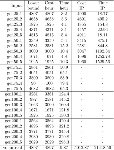
Table 5: Test results on size (5, 50, 75, 100, 200, real ) Input Lower
bound Cost heur
Time heur
Cost IP
Time IP
gen25 1 4807 4807 3.2 4900 18.77
gen25 2 4658 4658 3.6 4691 495.2
gen25 3 1825 1825 4.1 1855 154.8
gen25 4 4371 4371 3.1 4457 22.96
gen25 5 4815 4815 5.4 4911 18.11
gen50 1 3359 3359 5.4 3415 875.1
gen50 2 2581 2581 15.2 2581 844.8 gen50 3 3000 3000 10.4 3047 1102.34 gen50 4 1671 1671 4.8 1696 1252.78 gen50 5 1925 1925 10.3 1960 1529.56
gen75 1 2861 2861 50.9 - -
gen75 2 4051 4051 65.1 - -
gen75 3 3809 3809 88.9 - -
gen75 4 90 100 79.4 - -
gen75 5 4682 4682 65.3 - -
gen100 1 3261 3361 124.4 - -
gen100 2 987 2581 145.2 - -
gen100 3 1663 3000 160.4 - -
gen100 4 1671 1671 121.8 - -
gen100 5 1925 1925 130.3 - -
gen200 1 3564 3564 420.4 - -
gen200 2 4895 4895 321.2 - -
gen200 3 3771 3771 345.4 - -
gen200 4 2930 3930 329.8 - -
gen200 5 2029 2029 298.3 - -
volan real 4897 4897 9.87 5012.87 21418.56
The results of TPC are compared to the lower bound (see Section 4.1.1) and the solution of the IP, see Table 5. It can be stated that in most cases our algo- rithm produced low running time and good solutions for each test case. The time complexity is found much higher for the IP than the heuristic in all cases. Though heuristic can not guarantee optimal solution, but in practical situations the run- ning time is also an important aspect. However, as the problem size increased the running time of IP became unacceptable.
As the test cases have shown, the iteration number was high enough to reach the lower bound in most cases. The IP was running with a relative gap of 2% in a case of the generated input and 4% in a case of the real input which means the IP stopped when the actual solution was maximum of 2% and 4% distance from the optimal solution. The above fact explains why the costs of the IP are slightly higher than that of the TGPM.
The real input consisted of approximately 4000 shifts in a one month planning period, i.e. approximately 120-140 shift per each workday. The number of the working drivers in the final solution was 150. The results of the real input were tested with the integer programming model, the results of the IP can be found in the last row of the table. With the TPC the problem could be solved with the estimated number of drivers in every case. We obtained that TPC is able to handle relatively large inputs producing good quality feasible solutions in reasonable running time. Furthermore, in the majority of the test cases, our method has reached the theoretical lower bound.
6 Conclusion and future works
In this paper important aspects of the crew rostering in the scheduling of bus drivers were introduced. First a mathematical model of the problem was defined. Then we proposed the TPC method for the crew rostering problem, which is a proof of concept dealing with some general international regulations. In the initial phase a preliminary rostering is constructed. First the number of workers is estimated, then days-off patterns are generated, and a conflict graph is built. Lastly, to produce an initial rostering, the graph is colored with the estimated number of colors, where each color refers to an worker. In the second phase, a tabu search method recolors the graph to reduce the cost by minimizing the total undertime and overtime.
Our method has been tested with artificially generated and real life instances.
The real instances belongs to the local public transport company of Szeged. For moderate sized problems, the results of the presented algorithm have been compared to the solutions of the appropriate integer programming model and to a lower bound. TPC produced a satisfactory running time, reached the lower bound in most cases and returned a feasible solution in all cases. In the future the running time could be improved with other methods such as paralell programming and additional regulations could be taken into account in the conflict graph with additional edges, or with penalties in the objective function.
7 Acknowledgement
L´aszl´o Hajdu was supported by the project ”Integrated program for training new generation of scientists in the fields of computer science”, no EFOP-3.6.3- VEKOP- 16-2017-0002 (supported by the European Union and co-funded by the European Social Fund).
Attila T´oth acknowledges the support of the National Research, Development and Innovation Office - NKFIH Fund No. SNN-117879.
Mikl´os Kr´esz was supported by the ARRS project N1-0093 (Public call for financing the Slovenian part of bilateral Hungarian and Slovenian Cooperation with NKFIH National Research, Development and Innovation Office).
Mikl´os Kr´esz and L´aszl´o Hajdu gratefully acknowledge the European Commis- sion for funding the InnoRenew CoE project (Grant Agreement 739574) under the Horizon2020 Widespread-Teaming program, and the Republic of Slovenia (Invest- ment funding of the Republic of Slovenia and the European Union of the European Regional Development Fund), and the support of the EU-funded Hungarian Grant EFOP-3.6.2-16-2017-00015.
The authors thank Tisza Vol´an for the test data and the technical consulta- tion, and the anonymous referees whose detailed comments helped to improve the presentation of the paper.
References
[1] A. Wren, J. Rousseau. Bus driver scheduling: An overview. Com- put. Aided Sched. Pubilc Trahnsport., pages 173–187, 1995. DOI:
10.1007/978-3-642-57762-8 12.
[2] Abbink, Erwin, Albino, Luis, Dollevoet, Twan, Huisman, D., Rous- sado, Jorge, and Saldanha, Ricardo. Solving large scale crew schedul- ing problems in practice. Public Transport, 3:149–164, 06 2011. DOI:
10.1007/s12469-011-0045-x.
[3] Adamuthe, Amol and Bichkar, Rajan. Tabu search for solving personnel scheduling problem. InProceedings - 2012 International Conference on Com- munication, Information and Computing Technology, ICCICT 2012, pages 1–
6, 10 2012. DOI: 10.1109/ICCICT.2012.6398097.
[4] Alfares, Hesham K. Survey, categorization, and comparison of recent tour scheduling literature. Annals of Operations Research, 127(1):145–175, Mar 2004. DOI: 10.1023/B:ANOR.0000019088.98647.e2.
[5] Br´elaz, Daniel. New methods to color the vertices of a graph.Commun. ACM, 22(4):251–256, April 1979. DOI: 10.1145/359094.359101.
[6] Chen, Mingming and Niu, Huimin. A model for bus crew scheduling problem with multiple duty types. Discrete Dynamics in Nature and Society, 2012, 09 2012. DOI: 10.1155/2012/649213.
[7] Dantzig, G.B. A comment on edies traffic delays at toll booths. Operations Research, 2:339–341, 1954. DOI: 10.1287/opre.2.3.339.
[8] Elshafei, Moustafa and Alfares, Hesham K. A dynamic programming algorithm for days-off scheduling with sequence dependent labor costs. J. of Scheduling, 11(2):85–93, April 2008. DOI: 10.1007/s10951-007-0040-x.
[9] Ernst, A. T., Jiang, H., Krishnamoorthy, M., and Sier, D. Staff scheduling and rostering: A review of applications, methods and mod- els. European Journal of Operational Research, 153(1):3–27, 2004. DOI:
10.1016/s0377-2217(03)00095-x.
[10] Ernst, Andreas Tilman, Jiang, H, Krishnamoorthy, Mohan, and Sier, David.
Staff scheduling and rostering: a review of applications, methods and mod- els. European Journal of Operational Research, 153(1):3 – 27, 2004. DOI:
10.1016/S0377-2217(03)00095-X.
[11] Gamache, Michel, Hertz, Alain, and Ouellet, J´erˆome Olivier. A graph col- oring model for a feasibility problem in monthly crew scheduling with pref- erential bidding. Comput. Oper. Res., 34(8):2384–2395, August 2007. DOI:
10.1016/j.cor.2005.09.010.
[12] Garey, Michael R. and Johnson, David S. Computers and Intractability: A Guide to the Theory of NP-Completeness. W. H. Freeman & Co., New York, NY, USA, 1979. DOI: 10.2307/2273574.
[13] Glover, Fred and Laguna, Manuel.Tabu Search. Kluwer Academic Publishers, Norwell, MA, USA, 1997.
[14] Golumbic, M.C. Algorithmic graph theory and perfect graphs. Academic Press, San Diego, California,, 1980. DOI: 10.1016/c2013-0-10739-8.
[15] H., Dowling D. Krishnamoorthy M. Mackenzie and D., Sier. Staff rostering at a large international airport. Annals of Operations Research, 72:125–147, 1997. DOI: 10.1023/A:1018992120116.
[16] Hajos, G. ¨Uber eine art von graphen. Int. Math Nachrichten, 1957.
[17] Heil, Julia, Hoffmann, Kirsten, and Buscher, Udo. Railway crew scheduling:
Models, methods and applications.European Journal of Operational Research, 2019. DOI: https://doi.org/10.1016/j.ejor.2019.06.016.
[18] John J. Bartholdi, III. A guaranteed-accuracy round-off algorithm for cyclic scheduling and set covering.Operations Research, 29(3):501–510, 1981. DOI:
10.1287/opre.29.3.501.
[19] Kemeny, V. Argilan A. Toth B. David C. and Pongracz, G. Greedy heuristics for driver scheduling and rostering. Proc. 2010 Mini-Conference Appl. Theor.
Comput. Sci., pages 101–108, 2010.
[20] Lau, Hoong Chuin. On the complexity of manpower shift schedul- ing. Computers & Operations Research, 23(1):93–102, 1996. DOI:
10.1016/0305-0548(94)00094-o.
[21] Marx, Daniel. Graph colouring problems and their applications in scheduling.
Periodica Polytechnica Electrical Engineering, 48(1–2):11–16, 2004.
[22] Meisels, Amnon and Schaerf, Andrea. Modelling and solving employee timetabling problems. Annals of Mathematics and Artificial Intelligence, 39(1):41–59, Sep 2003. DOI: 10.1023/A:1024460714760.
[23] Mesquita, Marta, Moz, Margarida, Paias, Ana, and Pato, Mar- garida. A decompose-and-fix heuristic based on multi-commodity flow models for driver rostering with days-off pattern. European Journal of Operational Research, 245(2):423 – 437, 2015. DOI:
http://dx.doi.org/10.1016/j.ejor.2015.03.030.
[24] Nurmi, K., Kyng¨as, J., and Post, G. Driver rostering for bus transit companies.
Engineering Letters, 19(2):125–132, December 2011.
[25] O., Fukunaga A. Hamilton E. Fama J. Andre D. Matan and I., Nourbakhsh.
Staff scheduling for inbound call and customer contact centers. AI Magazine, 23(4):30–40, 2002.
[26] Shen, Yindong and Kwan, Raymond S. K. Tabu search for driver scheduling.
In Voß, Stefan and Daduna, Joachim R., editors,Computer-Aided Scheduling of Public Transport, pages 121–135, Berlin, Heidelberg, 2001. Springer Berlin Heidelberg. DOI: 10.1007/978-3-642-56423-9 7.
[27] Van den Bergh, Jorne, Belin, Jeroen, Bruecker, Philippe, Demeulemeester, Erik, and De Boeck, Liesje. Personnel scheduling: A literature review.
European Journal of Operational Research, 226:367385, 05 2013. DOI:
10.1016/j.ejor.2012.11.029.
[28] W.J. Kolen, Antoon, Karel Lenstra, Jan, H. Papadimitriou, Christos, and Spieksma, Frits. Interval scheduling: A survey. Naval Research Logistics, 54:530 – 543, 08 2007. DOI: 10.1002/nav.20231.