MŰHELYTANULMÁNYOK DISCUSSION PAPERS
INSTITUTE OF ECONOMICS, CENTRE FOR ECONOMIC AND REGIONAL STUDIES, HUNGARIAN ACADEMY OF SCIENCES - BUDAPEST, 2018
MT-DP – 2018/15
The best indexation of public pensions:
the point system
ANDRÁS SIMONOVITS
Discussion papers MT-DP – 2018/15
Institute of Economics, Centre for Economic and Regional Studies, Hungarian Academy of Sciences
KTI/IE Discussion Papers are circulated to promote discussion and provoque comments.
Any references to discussion papers should clearly state that the paper is preliminary.
Materials published in this series may subject to further publication.
The best indexation of public pensions: the point system
Author:
András Simonovits research advisor Institute of Economics
Centre for Economic and Regional Studies, Hungarian Academy of Sciences also Mathematical Institute of Budapest University of Technology
E-mail: simonovits. andras@krtk.mta.hu
August 2018
The best indexation of public pensions:
the point system András Simonovits
Abstract
We reconsider the problem of indexation of public pensions, emphasizing that similar contribution paths should imply similar benefit paths. This robustness criterion is only satisfied by full wage indexing, which in turn requires the politically unpopular reduction of the accrual rates. To minimize the redistribution from low-earning short-lived citizens to high-earning long-lived ones, progressive benefits should be introduced.
Keywords: public pensions, indexation, fairness
JEL-codes: D10, H55
A legjobb nyugdíjindexálás a pontrendszer Simonovits András
Összefoglaló
Újra megvizsgáljuk a társadalombiztosítási nyugdíjak indexálását, hangsúlyozva azt a követelményt, hogy hasonló járulékpályáknak hasonló járadékpályát kell adniuk. Ezt a robusztussági ismérvet csak a már megállapított nyugdíjak teljes bérindexálása elégíti ki, amely azonban a járadékszorzók politikailag népszerűtlen csökkentését igényli. Sőt, ez a módszer maximalizálja a jövedelem-újraelosztást a kiskeresetű rövid életűektől a nagykeresetű hosszú életűekhez. Ezért a teljes bérindexálás degresszív nyugdíjakat kíván.
Tárgyszavak: tb-nyugdíj, valorizálás, indexálás, pontrendszer, jövedelem-újraelosztás
JEL: D10, H55
point2 with B
The best indexation of public pensions:
the point system
by
Andr´as Simonovits
Institute of Economics, CERS, Hungarian Academy of Sciences also Mathematical Institute of Budapest University of Technology,
Budapest, T´oth K´alm´an 4, Hungary, 1097 July 25, 2018
Abstract
We reconsider the problem of indexation of public pensions, emphasizing that similar contribution paths should imply similar benefit paths. This robustness criterion is only satisfied by full wage indexing, which in turn requires the politically unpopular reduction of the accrual rates; moreover, maximizes the redistribution from low-earning short-lived citizens to high-earning long-lived ones. Therefore the application of full wage-indexing calls for progressive benefits.
Keywords: public pensions, indexation, fairness JEL-codes: D10, H55
1. Introduction
In modern economies, initial public pensionsare indexed (valorized) by wages and pen- sions in progressare indexed by various combination of prices and wages. In my opinion, in the pension literature, the indexation of public pensions have not received the atten- tion which it deserves. In this paper, I call attention to a number of conflicting aims and suggest that the point system is the best method.
In the short run, in a normal country, the issue of indexation of pensions on progress is almost irrelevant. The consumer price index is equal to about 102, the nominal wage index is 104. Who cares if the nominal pensions are increased by 2 or 4%, or their arithmetic average, 3%? A typical pensioner spends about 20 years in retirement, therefore, the annual 1–2% differences become 20–40% differences at the end and 10–
20% deviations during the whole period. The latter difference manifests itself both at the macro and the micro levels.
In a less normal country, where real wages increase or decrease by 5–10% a year, with a relative freedom from the GDP’s index, indexation matters even in the short- run. Just in Hungary, from 2016 to 2018, real net average wage grew by an astonishing 28% while the GDP only grew only by 10%, pensions even less than the GDP. Those, who retire in 2017–2019 receive pensions higher by 10–20–30% than those, who—with similar wage paths—retired in 2016. The whole story is described in Table 1.
The only method to avoid this anomaly is to raise pensions in progress by the nationwide wage growth rate, shortly: wage indexation. At the same time, this type of indexation makes the necessary reductions in the marginal accrual rate (transforming wages into initial benefits per contributive year) more visible and prefers those living longer (females and higher earners) and weakens the incentives to retire later. Finally, in a country, where the pension system is DC, some form of flat component is inevitable.
At this point I must admit that between 2010 and 2017 I also accepted the prevailing wisdom in Hungary: only pure price indexation is feasible.
Here we give a short review of the relevant literature. The best starting point is Barr and Diamond (2008, Subsection 5.1.4) which begins with the indexation of covered wages in calculating the initial benefits (valorization) and indexation of benefits in payment (or in progress). Concentrating on the latter, they analyze the advantages and disadvantages of price and wage indexation: the price indexing defends the workers against drop in real benefit; for a given starting value, it is less costly to the government than wage indexing but for growing real wages, it results in a relative decrease of pensions to wages: the earlier one retired, the more so. Price indexation is better for short lived pensioners than for others.
Feldstein (1990) created a very abstract and extravagant model of the socially op- timal age structure of the US Social Security benefits. Simonovits (2003, Section 14.4) modeled the intercohort impact of replacing wage indexation by price indexation. Legros (2006) analyzed the interaction of indexation and lifetime redistribution. Lovell (2009) gave a deep critique of the inconsistencies in US Social Security rules. Augusztinovics and Matits (2010); Borl´oi and R´eti (2010) worked out the point system with and without basic pension for Hungary. Weinzierl (2014) analyzed the impact of various price indices on the US Social Security system. Knell (2018) gave a deep critique of various versions of cohort-specific NDC rules, and numerically illustrated their approximate characters.
Table 1. Output, real wage and real pension dynamics: Hungary: 1993–2015 Real growth rate of Replacement
Year GDP net wage pension rate Comment
t 100(gy−1) 100(gw−1) 100(gb−1) ˆγt wage indexation
1993 –0.8 –3.9 –4.6 0.603
1994 3.1 7.2 –4.7 0.594 E: change in PIT
1995 1.5 –12.2 –10.1 0.619 change in delay
1996 0.0 –5.0 –7.9 0.593
1997 3.3 4.9 0.4 0.563
1998 4.2 3.6 6.2 0.578 E
1999 3.1 2.5 2.1 0.592
Swiss indexation (half wage+half price)
2000 4.2 1.5 2.6 0.591
2001 3.8 6.4 6.6 0.591 + raise
2002 4.5 13.6 9.8 0.573 E++ raise
2003 3.8 9.2 8.5 0.568 + 1 week pension
2004 4.9 –1.1 3.9 0.600 + 2 weeks pension
2005 4.4 6.3 7.9 0.611 + 3 weeks pension
2006 3.8 3.6 4.5 0.623 E + 4 weeks pension
2007 0.4 –4.6 –0.3 0.668
2008 0.8 0.8 3.4 0.691
2009 –6.6 –2.3 –5.7 0.672 no 13th month benefit
price indexation
2010 0.7 1.8 –0.9 0.651 E
2011 1.8 2.4 1.2 0.647
2012 –1.7 –3.4 0.1 0.670
2013 1.9 3.1 4.5 0.678 overindexation
2014 3.7 3.2 3.2 0.675 E+ overindexation
2015 2.9 4.3 3.5 0.668 overindexation
2016 2.1 7.4 1.4 0.631 start of wage explosion
2017 4.1 10.2 3.0 0.583 wage explosion continued
2018* 4.0 8.0 2.0 0.550 wage explosion ends
Source: ONYF (2016, Table 1.3, p. 16), new data are added, * forecast, E = election.
It was probably Liebmann (2002) who first documented that the apparently pro- gressive US Social Security system is hardly progressive on a lifetime basis, because life expectancy at retirement is an increasing function of the lifetime income. Recently there is a growing concern for this tendency which is strengthening. Among others, The Na- tional Academy ... (2015), Auerbach et al. (2017); Ayuso, Bravo and Holzmann (2017) reconsidered this problem on newer data. Simonovits (2018a, Section 14.4) returned to Legros’s topic: the impact of weight of wage in indexation on the redistribution from the short-lived low-paid to the long-lived high-paid.
The structure of the present paper is as follows. Section 2 discusses the advantages and disadvantages of price indexation, while Sections 3 and 4 analyze the point system at macro and microlevels, respectively. Section 5 concludes. Appendix A contains the pension formulas for wage paths different from the average path, while Appendix B analyzes a model where the forced reduction of the employer’s contribution rate temporary accelerates the real wage growth and strengthens inequalities between cohorts (Simonovits, 2018b).
2. Advantages and disadvantages of price indexation
In this paper, we calculate in real terms, i.e. we eliminate any inflationary effect. The only remaining problems stem from changes in the average real (total) wage.
In this Section, we create the core model. Lett be the index of year,vt andbt be the corresponding average net wage and benefit in real terms. Assuming a given aggregate accrual rate β (e.g. 0.8 for 40 years of contribution in Hungary), current initial benefit is proportional to past net wage:
bR,t=βvt−1. (1)
(N.B. We have neglected the impact of the changing relative value of the cap operat- ing.) General wage paths will be considered in Appendix A. Note that the valorization contains a one-year lag in a number of countries and this will create problem later on.
For price indexation, the benefit in progress retains its real value set at retirement:
bk,t=bk−1,t−1 =· · ·=βvt−k+R, k =R+ 1, . . . , D−1, (2) where D is an integer denoting life expectancy.
Neglecting the rises in life expectancy and in normal retirement age, and the vari- ability of the total fertility rate we have a stationary population. We assume that every pensioner (male or female) spends T = D−R years in retirement. Then the average benefit and the average replacement ratio are respectively equal to
¯bt = bR,t+· · ·+bD−1,t
T and γt = ¯bt
vt. (3)
Inserting (1) and (2) into (3):
γt =βvt−1+· · ·+vt−T
T vt . (4)
Dropping superscriptvfromgtv, letgt =vt/vt−1 be the real growth factor of average net wages. For the time being, assume that this growth factor is time-invariant, i.e.
vt =v0gt, g >1. (5)
Substituting (5) into (4) and using the formula for the sum of the geometric progression, we obtain
Theorem 1. For a constant real wage growth factor g, the corresponding constant replacement ratio is given by
γ =β g−1+· · ·+g−T
T =β 1−g−T
T(g−1), g > 1. (6)
Table 2 helps understanding a well-known disadvantage of price indexation: the higher the real growth rate, the lower the average replacement ratio with respect to the aggregate accrual rate. The lag in valorization (1) causes a small part of the drop, and the lagging of pensions in progress behind the initial one in indexation (2) causes the large part of the drop. Quantitatively, with T = 20 year, Table 2 demonstrates how the replacement ratio drops from 0.8 through 0.6 to 0.5 as the growth rate rises from 0 through 3 to 5%.
Table 2. Average replacement ratio and growth rate of real wage
Growth rate of real wage 100(g−1) % 0 1 2 3 4 5
Average replacement ratio γ 0.800 0.722 0.654 0.595 0.544 0.498 Turning to the more realistic time-variant growth rates, a more complex picture emerges. We shall derive a recursion connecting the new replacement ratio with the past replacement ratio and other factors.
Representing every cohort by a single pensioners, the change in the pension expen- diture is connected by the change in the stock of pensioners:
T¯bt =bt +T¯bt−1−bt−T. (7) Hence relying on (4), the average replacement ratio is given by
γt = ¯bt
vt = ¯bt−1
gtvt−1 +βvt−1−vt−T−1
T vt . (8)
We introduce the accumulated real wage growth factor between years t−T and t:
Gt = vt/vt−T which is also equal to the ratio of the next year’s youngest and oldest pensions: Gt =bt+1/bt−T+1. (8) implies
Theorem 2. For time-variant growth rates, the dynamic of replacement ratio is given by
γt = γt−1
gt
+β1−G−1t−1
gtT , t = 0,1,2, . . . . (9) It is worth adding some explanation to formula (9). The second term is less than β/T = 0.04, which pushes up or down the slightly contracted past replacement ratio.
Having this formula, we model the impact of the extraordinary wage rises occurring in Hungary during 2016–2018 on the average replacement ratio. We assume that there
are two values of the real wage growth factors 1 < gm < gM, the greater is reached in year t0−1, t0, t0+ 1:
gt =
½gm if t < t0−1 or t > t0+ 1;
gM, otherwise.
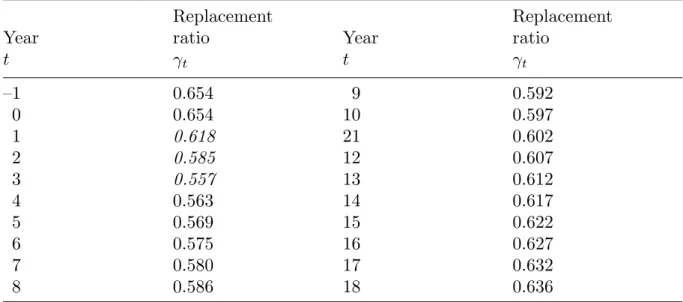
Noting that G0 =gmT and γ1 = γ(gm) and working with gm = 1.02 and gM = 1.08, Table 3 depicts a stylized process. Starting from a steady state, the wage explosion reduces γ0 = 0.654 to γ3 = 0.557 and then γt slowly rises again.
Table 3. Dynamics of replacement ratio with price indexation
Replacement Replacement
Year ratio Year ratio
t γt t γt
–1 0.654 9 0.592
0 0.654 10 0.597
1 0.618 21 0.602
2 0.585 12 0.607
3 0.557 13 0.612
4 0.563 14 0.617
5 0.569 15 0.622
6 0.575 16 0.627
7 0.580 17 0.632
8 0.586 18 0.636
It is natural that the temporary drop of the average replacement ratio makes room for a similar temporary reduction of the contribution rate. But as the replacement ratio returns to its formal state, so does the contribution rate.
Finally, we present two simple though artificial examples showing the pitfalls of pure price indexation and fixed accrual rate.
Example 1. Start from the life path of citizen X, who worked 40 years before retired on the last day of year t, at the normal retirement age R. She will receivebXR,t= βvt−1. Her twin brother Y, retired one day later, with the same wage path with benefit bYR,t=βvt. If vt > vt−1, then bYR,s = (vt/vt−1)bXR,s > bXR,s, for s=t+ 1, . . . , t+D−R, just for an extra day of contribution.
The second example is much more robust than the first one.
Example 2. Let us assume that the real net wage is equal tovm in even years, and to vM in odd years, vm < vM. X starts to work in an even year; Y, who is one year younger, in an odd year. Both earn the annual average net wage during their careers.
Since both work for 40 years, X retires in an even year, while Y does the same in an odd year and the previous anomaly is repeated: bXt = βwm and bYt = βwM. If wage indexation were in force, then the benefits would be bX2t = 0.8vM and bY2t+1 = 0.8vm, but the last year’s benefit of Y is again bX2t = 0.8vM, when X is already dead. The total benefits are the same.
3. Point system at macrolevel
We still consider the macroworld. We have already seen that with wildly oscillating real wages, the price indexation of pensions in progress is strongly unfair across cohorts. We add now: the partial wage indexation only dampens but does not eliminate unfairness.
We have to answer the following question: why did the Hungarian government give up wage indexation in 2000, and the wage-price indexation in 2010? The answer is simple:
for fast rising real wages, the fixed accrual rate have exploded the pension expenditures, especially when the fast aging population and slowily increasing average retirement age are also taken into account. Of course, the government could have reduced the accrual rate from 0.8 to 0.657 (consistent with g = 1.02) as suggested by Table 2 but it would have been difficult politically to do so. Furthermore, to dampen the impact of the more economical wage-price indexation, a 13th month pension was phased in between 2003–2006 (cf. Table 1 above).
Now we model the point system. To make room for the contribution and personal income tax rates, we rewrite the previous net wage equation for total rather than net wage (superscript w is also omitted):
wt =gtwt−1. (10)
Since we fix the pension contribution rate τ and the sum of the health contribution rate and the personal income tax rate,θ, the real value of the net income also grows in parallel:
vt = (1−τ −θ)wt and vt =gtvt−1.
We delay the formal definition of the point system to Appendix A, here we depict it as a simultaneous wage valorization and indexation. Anyway, we get rid of the lag in (1) as well as in (2).
Valorization of the initial pension with adjustable gross aggregate accrual rate:
bR,t= ˜βtwt. (11)
Indexation of pensions in progress:
bR+k,t = ˜βtwt, k = 1, . . . , T −1. (12)
Denoting by Pt the number of pensioners, the pension expenditure is given by
Bt =Ptβ˜twt. (13)
Denoting by Mt the number of workers, the pension revenue is also equal to
Bt =τ Mtwt. (14)
Comparing (13) and (14) yields
τ Mt =Ptβ˜t. Introducing the old-age dependency ratio
πt = Pt
Mt, simple calculation yields
Theorem 3. For a point system, the adjustable gross and net accrual rates are respectively given by
β˜t = τ
πt and βt = β˜t
1−τ −θ = τ
(1−τ−θ)πt. (15) b) The benefit is independent of the year of retirement: bt =βtvt.
Introducing the point system, we maintained the balance of the system and avoided the intercohort unfairness of price indexation. Note that this rule does not prevent a drop in the benefit when the accrual ratio or the net wage drops. If we set up a trust fund, then the following feedback rule helps avoiding any drop:
bt =
(βtvt, if βtgt ≥βt−1 and bt−1 > bt−2; βtvt+κFt−1 if βtgt ≥βt−1 and bt−1 =bt−2; bt−1, otherwise,
where κ >0 is an appropriately chosen feedback coefficient. The trust fund’s dynamics is as follows:
Ft =Ft−1+τ Mtwt−Ptbt, F0 = 0. (16) This rule has nothing to do with the overindexation rule which used the greater of 1 or the real wage growth factor and operated in the UK between 1975 and 1980 (Barr–Diamond, 2008, Box 5.8, p. 77).
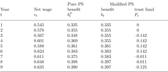
To demonstrate the operation of our rule, we use the following parameter values as of Hungary, 2018. Pension contribution rate: τ = (0.1 + 0.145)/1.195 = 0.205; health + unemployment+PIT rate: θ = (0.135 + 0.15)/1.195 = 0.238; i.e. with a dependency ratio π = 0.6, the gross and net replacement ratios are respectively equal to ˜β = 0.342 and β = 0.342/(1−0.205−0.238) = 0.614.
Table 4 displays the following dynamic when the growth factor is given as gt = 1.02 + (−1)t0.04, i.e. it alternates between 0.98 and 1.06, their geometric average being close to 1.02. Note that without the trust fund, from year 2 to year 3, in terms of the initial gross wage, the benefit drops from 0.355 to 0.348. In the modified system, in odd years, the benefit remains the same as previously, but in even years, its value is diminished with respect to the simple rule, e.g. in year 4, 0.355<0.369. The trust fund value oscillates with narrow bounds.
Table 4. Point systems (PS) without or with trust fund
Pure PS Modified PS
Year Net wage benefit benefit trust fund
t vt bPt bt Ft
1 0.545 0.335 0.335 0
2 0.578 0.355 0.355 0
3 0.567 0.348 0.355 –0.142
4 0.601 0.369 0.355 0.142
5 0.588 0.361 0.361 0.142
6 0.624 0.383 0.383 0.142
7 0.611 0.375 0.383 –0.011
8 0.648 0.398 0.397 0.011
9 0.635 0.390 0.397 –0.125
4. Point system at microlevel
In Sections 2 and 3, we demonstrated that at the macro-level, the only consistent method is wage indexation with an adjusted accrual ratio. This requires, however, some political courage from the government. Moreover, at micro-level, wage indexation has a very unpleasant side effect: since the life expectancies of various income groups widely differ, namely higher earners live longer, then the faster the benefits increase, the stronger the income redistribution from the shorter lived to the longer lived. This can only be mitigated by pension progression or return to progressive personal income taxation.
Working out the necessary changes, for simplicity, we neglect now the time-variance of real wage growth factors but relax the assumptions of homogeneous wages and life expectancies. (For a more general description, see Appendix A.) Let i be the index of group i, fi > 0 be their initial frequency: Pn
i=1fi = 1 and wi,t be the corresponding wage:
wi,t=wi,0gt, where Xn
i=1
fiwi,0 = 1. (17)
By assumption, everybody retires at age R, type i lives until Di: Di is increasing, and Pn
i=1fiDi =D.
It would be a simple solution to have type-specific accrual rates βi (i= 1,2, . . . , n) but it would be politically untenable. Rather, we rely on progression or equalize part of the DC benefits. Denoting average total and net wages by wt and vt, respectively, the share of proportional benefits be α, 0≤α≤1.
Then the point rule provides the mixed benefits:
bi,k,t= ˜β[αwi,t+ (1−α)wt], k =R, . . . , D−1. (18)
Simplifying the calculations, we retain stationary population, and introduce the common length of contribution S =R−Q. The balance condition is now
τ Swt = Xn
i=1
fiTibi,t.
Take the simply and doubly weighted average times spent in retirement respectively:
T = Xn
i=1
fiTi and Tw = Xn
i=1
fiTiwi,0. (19)
Obviously, Tw > T. Substituting (18) and (19) into the first balance condition, yields the second balance equation:
τ S= Xn
i=1
fiTiβ[αw˜ i,t+ (1−α)wt].
Thus we have arrived to
Theorem 4. (a) For heterogeneous wage profile (wi,0) and times (Ti) spent in retirement, the balanced gross and net accrual rates are respectively equal to
β˜α = τ S
αTw + (1−α)T and βα = β˜α
1−θ−τ. (20)
Remark. As the proportional benefit’s shareαdecreases, so rises the accrual rate.
The proportion of the two extreme cases (0/1) is equal to Tw/T, and this also increases with heterogeneity.
We shall analyze the income redistribution due to heterogeneous earnings and life expectancies. Corresponding to the logic of the pay-as-you-go system, the type-specific lifetime balance in year 0 should be discounted by the real growth factor g, therefore it is defined by
zi =τ Swi,0−
Di
X
k=R
g−(k−R)bi,k,k.
Using (19), the balance is given by
zi =τ Swi,0−β[αT˜ iwi,0+ (1−α)Ti]. (21) As an illustration , we consider the traditional homogeneous case, where Ti ≡ T, i.e. Tw = T, i.e. (20) is replaced by ˜β =S/T, regardless α. The type-specific lifetime balance is equal tozi=τ S(1−α)(wi,0−1), i.e. those who earn below the average, gain (zi <0), the others lose (zi >0).
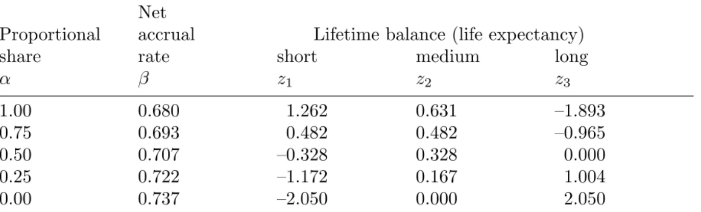
Table 5 presents a numerical example. There are three types: w1,0 = 0.5; w2,0 = 1 and w3,0 = 1.5; their frequencies are 1/3. Let the corresponding life expectancies be D1 = 75, D2 = 80, and D3 = 85, Though their average is D = 80, the lower the proportional part, the higher the accrual rate. In addition, we display the life balances.
For a proportional system (α = 1), the higher earners and longer lived are the gainers (z3 <0), the others are the losers; this changes with decreasing α.
Table 5. Progression, accrual rates and balances Net
Proportional accrual Lifetime balance (life expectancy)
share rate short medium long
α β z1 z2 z3
1.00 0.680 1.262 0.631 –1.893
0.75 0.693 0.482 0.482 –0.965
0.50 0.707 –0.328 0.328 0.000
0.25 0.722 –1.172 0.167 1.004
0.00 0.737 –2.050 0.000 2.050
Note that we have left out the fragmentation of working careers (cf. Augusztinovics and K¨oll˝o, 2007) and here we make up this omission. We introduce the simple and double-weighted expected contribution lengths, respectively:
S = Xn
i=1
fiSi and Sw = Xn
i=1
fiwi,0Si. Now (20)–(21) modify into
β˜α = τ Sw
αTw+ (1−α)T and
zi =τ Siwi,0−β[αT˜ iwi,0+ (1−α)Ti].
We have also neglected early and late retirement, these problems have been analyzed in other papers (e.g. Czegl´edi, Simonovits, Szab´o and Tir, 2017 and Simonovits, 2018a).
5. Conclusions
At the end of the paper, we draw some conclusions. We have demonstrated that the apparently economical partial wage indexing or pure price indexation has a number of pitfalls. In addition to reducing the relative value of old benefits to current wages, it also creates unjustified differences between pension paths of close earning paths, especially for temporarily exploding real wages. This anomaly justifies a return to or the introduction of wage indexation, but the accrual rate of the initial benefits should be controlled. We have to realize the pitfall of the wage indexation that it maximizes the perverse redistribution from low-earning short lived citizen to high-earning long-lived ones. To mitigate this pitfall, we have to return to progressive pensions or progressive personal income taxation.
Unfortunately, introducing progression weakens the incentives to report wages. In addition, together with wage indexation, they weaken the incentives to work longer and strengthen those for early retirement. But the wage indexation is the smallest bad if supplemented with progression.
Appendix A. Valorization, indexation and point system
In the main text we avoided structurally changing time-variant real wage developments.
Now we make up this omission.
Assume that a worker of typei, born in year t enters work at ageQand earns a net real wage vi,a,t+a at age a, a=Q, . . . , R−1. Neglecting the implied net wage cap, her initial pension is given as
bi,R,t+R =δt+R R−1X
a=Q
Gt+R−1,avi,a,t+a, (A.1)
where the valorization multipliersfrom age a to year t+R in real terms are Gt+R−1,a = vt+R−1
vt+a , a=Q, . . . , R−1,
where vt+a is the nationwide net real wage in yeart+a and δt+R denotes the marginal accrual rate.
Letι be a real number between 0 and 1, which shows the weight of the wage growth on the benefit in progress, then
bi,a,t+a =bi,a−1,t+a−1gtι, a=R+ 1, . . . , D−1. (A.2) It is obvious that ι = 1,1/2,0 represent wage, wage-price and price indexation, respectively.
In year t+a, an i-type worker of age a earns points pi,a,t+a = vi,a,t+a
vt+a , (A.3)
i.e. the ratio of her net wage to the nationwide average. Her accumulatedpoints earned up to retirement is equal to the sum of these points:
pi,R,t+R=
R−1X
a=Q
pi,a,t+a. (A.4)
The value of one point in yeart+a, xt+a is determined by the government through the balance condition, yielding a benefit path
bi,a,t+a =pi,R,t+Rxt+a, a=R, . . . , D−1. (A.5) Note that in the point system there is neither wage indexation nor price indexation nor their mixture; the benefit rise xt+a/xt+a−1 is determined from two complex balance conditions.
Appendix B. Forced reduction of pension contribution rate
This Appendix discusses three scenarios for the forced reduction of pension contribution rate concerning current Hungarian developments. To do so we have to introduce the gross wage u, the total wage compensation w and break down the pension and health contribution rates between employee’s (E) and employer’s (firm F) rates: Let θE and θF be the exogenously given and constant health care contribution rates paid by the employee and the employer (the former also includes the personal income tax rate), respectively. Let τE and τtF be the exogenously given pension contribution rates paid by the employee and the employer, respectively, their sum being the pension contribution rate τt =τE +τtF—the latter two being time-variant. By definition, for a given gross wage ut, the total and the net wages in yeart are respectively equal to
wt = (1 +θF +τtF)ut (B.1)
and
vt = (1−θE−τE)ut, ahol θE+τE <1. (B.2) Reflecting the logic of the current Hungarian pension system, the initial representative benefit in year t is proportional to the net representative wage in year t − 1 and to time-varying length of contributions St:
bt =δStvt−1. (B.3)
(Appendix A explains why this does not apply to individual benefits.)
Due to the price indexation of benefits in progress, in year t (in real terms) the representative benefit set k−1 years earlier is still equal to
bt−k =δStvt−k, k = 2, . . . , T. (B.4) We assume that the length of the contribution period rises for a while:
St = 33 + 0.5(t−2016) if t= 2016, 2017, 2018 and St = 35 later. (B.5) Furthermore, pension revenues are given as
Rt =τtStut. (B.6)
Also, we diminish the entry of new pensioners by half until 2022, represented by multiplier at in (14) below, (an ad hoc assumption). To get rid of the complex problem of age distribution of benefits in 2016 granted k = 1,2, . . . , T years earlier, we model the pension expenditures like
Bt =Bt−1+δ(atStvt−1−S2015v2015). (B.7) The parameter values are as follows: τE = 0.10, τ−1F = 0.22, θE = 0.15 + 0.085 = 0.235 and θF = 0.05, with T = 20 years, the annual accrual rate δ = 0,023. We choose at = 0.7 until 2022, later it rises to 1.
We compare three scenarios: Scenario 1 depicts the forced reduction of pension contribution rate as a feasible process due to high wage growth. Scenario 2 describes the process as infeasible due to slower wage growth. Scenario 3 stops the forced reduction to maintain the equilibrium. The numbers are given in percent. Revenues and expenditures are given in terms of the initial revenue.
Scenario 1. Persistently fast wage growth and fast reduction of pension contribution rate
The first scenario (displayed in Table B.1) is consistent with the government plan but it assumes very fast real total wage growth, namely 5% per year. We assume that τtF drops from 0.22 (t =−1) to 0.085. Here are the numerical results.
Table B.1.
Persistently fast wage growth and fast reduction of pension contribution rate, % Pension contrib- Real growth rate P e n s i o n
Year ution rate of total wage revenues expenditures
t 100τt 100(gwt −1) 100Rt/R2016 100Bt/R2016
2016 32.0 7.4 100.0 95.6
2017 27.0 5.9 94.4 94.5
2018 24.5 5.8 93.9 93.9
2019 22.5 5.2 93.6 93.6
2020 20.5 5.2 91.3 93.6
2021 18.5 5.1 88.1 93.9
2022 18.5 5.1 92.5 94.6
2023 18.5 5.0 97.2 97.8
2024 18.5 5.0 102.0 101.4
2025 18.5 5.0 107.1 105.3
Scenario 2. Decelerating wage growth and fast reduction of pension contri- bution rate
The second scenario (Table B.2) reduces the total wage growth rate to a feasible value namely 3% starting with 2019 but the government continues its reduction program.
(The data of years 2016–2018 are the same as in Table B.1, therefore they are omitted.) Then the gap between the revenues and the expenditures widens and by 2022 reaches 8% of the initial revenues, amounting to 1% of the GDP.
Table B.2.
Decelerating wage growth and fast reduction of pension contribution rate, % Pension contrib- Real growth rate P e n s i o n
Year ution rate of total wage revenues expenditures
t 100τt 100(gwt −1) 100Rt/R2016 100Bt/R2016
. . . . . .
2019 22.5 3.2 91.9 93.6
2020 20.5 3.2 87.9 93.5
2021 18.5 3.2 83.3 93.7
2022 18.5 3.0 85.8 94.0
2023 18.5 3.0 88.3 96.7
2024 18.5 3.0 91.0 99.5
2025 18.5 3.0 93.7 102.6
Scenario 3. Decelerating wage growth and reduction of pension contribution rate
The third scenario (Table B.3) adjusts the pension contribution rate to the decelerating total real wage growth. Stopping at 20.5 rather than 18.5, the equilibrium is more or less preserved.
Table B.3.
Decelerating wage growth and pension contribution rate, % Pension contrib- Real growth rate P e n s i o n
Year ution rate of total wage revenues expenditures
t 100τt 100(gwt −1) 100Rt/R2016 100Bt/R2016
. . . . . .
2019 22.5 3.2 91.9 93.6
2020 20.5 3.2 87.9 93.5
2021 20.5 3.0 90.5 93.7
2022 20.5 3.0 93.2 93.9
2023 20.5 3.0 96.0 96.4
2024 20.5 3.0 98.9 99.2
2025 20.5 3.0 101.9 102.1
Even this scenario maintains a distorted pension profile where the benefits of those who retired in 2019 are cc. 28% higher than the benefits of those who retired in 2016.
Note that these runs are quite primitive and further examinations are needed to corroborate their robustness.
References
Auerbach, A. et al. (2017): “How the Growing Gap in Life Expectancy may Affect Retirement Benefits and Reforms,” NBER WP 23329, Cambridge, MA.
Augusztinovics, M. and K¨oll˝o, J. (2008): “Pension Systems and Fragmented Labor Market Careers,” G´al, R. I., Iwasaki, I. and Sz´eman, Zs., eds. Assessing Intergen- erational Equity,154–170.
Augusztinovics, M. and Matits, ´A. (2010): “Point System and Basic Pension: A Frame- work for Old-age Pension Reform”,Report on the Pension and Old-age Round Table (in Hungarian), Budapest, Hungarian Government, ed. by P. Holtzer, 234–246.
Ayuso, M., Bravo, J. M. and Holzmann, R. (2017): “Addressing Longevity Heterogene- ity in Pension Scheme Design and Reform”,Journal of Finance and Economics, 6, 1–21.
Barr, N. and Diamond, P. (2008): Reforming Pensions: Principles and Policy Choices, Oxford, Oxford University Press.
Borl´oi, R. and R´eti, J. (2010): “The Point System Paradigm”, Report on the Pension and Old-age Round Table (in Hungarian), Budapest, Hungarian Government, ed.
by P. Holtzer, 218–233.
Czegl´edi, T.; Simonovits, A.; Szab´o, E. and Tir, M. (2017): “What has been Wrong with the Retirement Rules in Hungary?”, Acta Oeconomica 67, 359–387.
Feldstein, M. S. (1990): “Imperfect Annuity Markets, Unintended Bequest, and the Optimal Age Structure of Social Security Benefits”, Journal of Public Economics 41,31–43.
Holzmann, R. and Palmer, E. eds. (2006): Pension Reforms: Issues and Prospects of Nonfinancial Defined Contribution (NDC) Schemes. Washington, D.C., World Bank.
Knell, M. (2018): “Increasing Life Expectancy and NDC Pension Systems”, Journal of Pension Economics and Finance 17:2,170–199. o.
Legros F. (2006): “NDCs: A Comparison of French and German Point Systems,” Holz- mann and Palmer, eds. 203–238.
Liebmann, J. B. (2002): “Redistribution in the Current U.S. Social Security System”, Feldstein, M.A. and Liebmann, J.B. eds.: The Distributional Aspects of Social Se- curity and Social Security Reform, Chicago, Chicago University Press, 11–48.
Lovell, M. (2009): “Five OAIAS Inflation Indexing Problems”, Economics: Open Ac- cess, Open Assessment E-Journal, 3.
National Academies of Sciences, Engineering, and Medicine (2015): The Growing Gap in Life Expectancy by Income: Implications for Federal Programs and Policy Re- sponses, The National Academics Press, Washington D.C.
ONYF (2016): ONYF–2015 Statistical Yearbook, in Hungarian, Budapest.
R´ezmovits, ´A. (2015): “The Comparative Analysis of Pension Benefit Rules”,Economic Review, 62(in Hungarian), 1309–1327.
Simonovits, A. (2003): Modeling Pension Systems, Houndsmill, Basingstoke, Palgrave, Macmillan.
Simonovits, A. (2018a): Simple Models of Income Redistribution. Oxford, Palgrave- MacMillan.
Simonovits, A. (2018b): Forced pension contribution rate? IE-CERS-HAS Working Papers 18.
Weinzierl, M. (2014): “Seesaws and Social Security Benefits Indexing”, Brookings Pa- pers on Economic Activity, Fall,137–196.
Whitehouse, E. and Zaidi, A. (2008): “Socioeconomic Differences in Mortality: Im- plications for Pension Policy”, OECD Social, Employment and Migration Working Papers 70, Paris, OECD.