Resources: Minimizing the Sum of Completion Times

Resources: Minimizing the Sum of Completion Times

Krist´of B´erczi¹, Tam´as Kir´aly¹⁽B⁾, and Simon Omlor²

1 MTA-ELTE Egerv´ary Research Group, Department of Operations Research, E¨otv¨os Lor´and University, Budapest, Hungary

{berkri,tkiraly}@cs.elte.hu

2 Institute for Algorithms and Complexity, TU Hamburg, Hamburg, Germany simon.omlor@tuhh.de

Abstract. We consider single-machine scheduling problems with a non- renewable resource. In this setting, there arenjobs, each characterized by a processing time, a weight, and a resource requirement. At given points in time, certain amounts of the resource are made available to be consumed by the jobs. The goal is to assign the jobs non-preemptively to time slots on the machine, so that each job has the required resource amount available at the start of its processing. We consider the objective of minimizing the weighted sum of completion times.

The main contribution of the paper is a PTAS for the case of 0 processing times (1|rm = 1, pj = 0|

wjCj). In addition, we show strong NP-hardness of the case of unit resource requirements and weights (1|rm= 1, aj = 1|

Cj), thus answering an open question of Gy¨orgyi and Kis. We also prove that the schedule corresponding to the Shortest Processing Time First ordering provides a 3/2-approximation for the latter problem.

Keywords: Scheduling

·

·

·

Approximation algorithm

1 Introduction

Scheduling problems with non-renewable resource constraints arise naturally in various areas where resources like raw materials, energy, or funding arrive at predetermined dates. In the general setting, we are given a set of jobs and a set of machines. Each job is equipped with a requirement vector that encodes the needs of the given job for the different types of resources. There is an initial stock for each resource, and some additional resource arrival times in the future are known together with the arriving quantities. The aim is to find a schedule of the jobs on the machines such that the resource requirements are met.

Supported by DAAD with funds of the Bundesministerium f¨ur Bildung und Forschung (BMBF) and by DFG project MN 59/4-1.

c Springer Nature Switzerland AG 2020

M. Ba¨ıou et al. (Eds.): ISCO 2020, LNCS 12176, pp. 167–178, 2020.

https://doi.org/10.1007/978-3-030-53262-8_14

We will use the standard α|β|γ notation of Graham et al. [5]. Grigoriev et al. [6] extended this notation by adding the restriction rm = r to the β field, meaning that there arer resources (raw materials). In the present paper, we concentrate on problem 1|rm = 1|

w_jC_j, that is, when we have a single machine, a single resource, and the goal is to minimize the weighted sum of completion times.

Previous Work. Scheduling problems with resource restrictions (sometimes called financial constraints) were introduced by Carlier [2] and Slowinski [16].

Carlier settled the computational complexity of several variants for the single machine case [2]. In particular, it was shown that 1|rm= 1|

wjCj is NP-hard in the strong sense. This was also proved independently by Gafarov, Lazarev and Wener in [3]. Kis [15] showed that the problem remains weakly NP-hard even when the number of resource arrival times is 2 and gave an FPTAS for 1|rm = 1, q = 2|

w_jC_j. A further variant of the problem was considered in [3]. Recently, Gy¨orgyi and Kis [13,14] gave polynomial time algorithms for several special cases, and also showed that the problem remains weakly NP-hard even under the very strong assumption that the processing time, the resource requirement and the weight are the same for each job. They also provided a 2-approximation algorithm for this variant. For a constant number of resource arrival times, they gave a PTAS when the processing time equals the weight for each job, and an FPTAS when the resource requirements and weights are 1.¹

In comparison, much more is known about the maximum makespan and maximum lateness objectives. Slowinski [16] studied the preemptive schedul- ing of independent jobs on parallel unrelated machines with the use of addi- tional renewable and non-renewable resources under financial constraints. Toker et al. [17] examined a single-machine scheduling problem under non-renewable resource constraint using the makespan as a performance criterion. Xie [18]

generalized this result to the problem with multiple financial resource con- straints. Grigoriev et al. [6] presented polynomial time algorithms, approxima- tions and complexity results for single-machine scheduling problems with unit or all-equal processing times. In a series of papers [7–11], Gy¨orgyi and Kis presented approximation schemes and inapproximability results both for single and paral- lel machine problems with the makespan and the maximum lateness objectives.

In [12], they proposed a branch-and-cut algorithm for minimizing the maximum lateness.

Our Results. The first problem that we consider is 1|rm = 1, aj = 1|

Cj. The complexity of this problem was posed as an open question in [12]. We show that the problem is NP-hard in the strong sense.

Theorem 1. 1|rm= 1, a_j= 1|

C_j is strongly NP-hard.

Given any scheduling problem on a single machine, theShortest Processing Time First (SPT) schedule orders the jobs by processing times, i.e.p_spt⁻¹(i)≤

1 Just before the submission of the present paper, Gy¨orgyi and Kis published an updated version of [14] with some new results. None of our results are implied by their paper.

p_spt⁻¹_(i+1)for alli. We prove thatsptprovides a 3/2-approximation. We remark that it remains open whether the problem is APX-hard.

Theorem 2. The SPT schedule gives a ³₂-approximation for 1|rm = 1, aj = 1|

Cj, and the approximation guarantee is tight.

The second problem considered is the special case when the processing time is 0 for every job. This setting is relevant to situations where processing times are negligible compared to the gaps between resource arrival times, and the bot- tleneck is resource availability. Examples include financial scheduling problems where the jobs are not time consuming but the availability of funding varies in time, or production problems where products are shipped at fixed time intervals and production time is negligible compared to these intervals. Note that the number of machines is irrelevant if processing times are 0.

First we present a PTAS for constant number of resource arrival times. This procedure will be used as a subroutine in our algorithm for the general case.

Theorem 3. There exists a(1+^q_k)-approximation for1|rm= 1, pj= 0|

Cjwj

with running time O(n^qk+1).

The main contribution of the paper is a PTAS for the same problem with an arbitrary number of resource arrival times.

Theorem 4. There exists a PTAS for1|rm= 1, pj= 0| Cjwj.

A peculiarity of the algorithm is that the PTAS for constant number of arrival times is called repeatedly on overlapping time windows, and at each call we fix only a portion of the scheduled jobs.

Due to space constraints, several proofs and details as well as further results are deferred to the full version of this paper, which is available at http://arxiv.

org/abs/1911.12138.

2 Preliminaries

Throughout the paper, we will use the following notation. We are given a set J of n jobs. Each job j ∈ J has a non-negative integer processing time pj, a non-negative weight wj, and a resource requirementaj. Theresources arrive at time points t1, . . . , tq, and theamount of resource that arrives at ti is denoted bybi. We might assume that_q

i=1bi =_n

j=1aj holds. We will always assume that t1= 0, as this does not effect the approximation ratio of our algorithms.

The jobs should be processed non-preemptively on a single machine. Asched- ule is an ordering of the jobs, that is, a mappingσ : J →[n], where σ(j) =i means that jobj is theith job scheduled on the machine. Thecompletion time of jobjin scheduleσis denoted byC_j^σ. We will drop the indexσif the schedule is clear from the context. In any reasonable schedule, there is an idle time before a jobjonly if there is not enough resource left to start jafter finishing the last job before the idle period. Hence, the completion time of job j is determined by the ordering and by the resource arrival times, as j will be scheduled at the earliest moment when the preceding jobs are already finished and the amount of available resource is at leastaj.

3 The Problem 1 |rm = 1 , a

= 1 | C

3.1 Strong NP-completeness

Proof of Theorem 1.Recall that alla_j andw_j values are 1, and each job has an integer processing timepj. The number of resource arrival times is part of the input. We prove NP-completeness by reduction from the3-Partitionproblem.

The input contains numbersB ∈N,n∈N, andxj ∈N(j = 1, . . . ,3n) such that B/4< xj< B/2 and3n

j=1xj =nB. A feasible solution is a partitionJ1, . . . , Jn

of [3n] such that|Ji|= 3 and

j∈Jixj =B for every i∈[n]. In contrast to the Partitionproblem, the3-partitionproblem remains NP-complete even when the integersxj are bounded above by a polynomial inn. That is, the problem remains NP-complete even when the numbers in the input are represented as unary numbers [4, pages 96–105 and 224].

LetK= 4nB. The reduction to 1|rm= 1, a_j= 1|

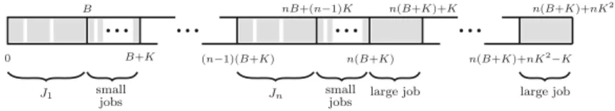
C_j involves three types of jobs.Normal jobscorrespond to the numbersx_jin the3-Partitioninstance, so there are 3nof them and the processing timep_j of thej-th normal job isx_j. We further havenK small jobs with processing time 1, andnKlarge jobs with processing time K. There are also three types of resource arrivals. The Type 1 resource arrival times are i(B +K) (i = 0, . . . , n−1) with three resources arriving at each. The Type 2 arrival times are i(B+K) +j (i= 0, . . . , n−1, j =B, . . . , B+K−1) with one resource arriving. Finally, theType 3 resource arrival times aren(B+K) +iK(i= 0, . . . , nK−1) with one resource arriving.

Suppose that the 3-Partition instance has a feasible solution J1, . . . , Jn. We consider the following schedule S: resources of Type 1 are used by normal jobs, such that jobs inJiare scheduled between (i−1)(B+K) andiB+ (i−1)K (in sptorder). Type 2 resources are used by small jobs that start immediately.

Type 3 resources are used by the large jobs that also start immediately at the resource arrival times (see Fig.1).

Instead of

C_j, we consider the equivalent shifted objective function (C_j− t_j−p_j), wheret_j is the arrival time of the resource used by job j andp_j is its processing time – we assume without loss of generality that resources are used by jobs in order of arrival. Note that all terms of

(C_j−t_j−p_j) are nonnegative. As small jobs and large jobs start immediately at the arrival of the corresponding resource in schedule S, their contribution to the shifted objective function is 0. The jobs in J_i have total processing time B, and their contribution to the shifted objective function is two times the processing time of the shortest job plus the processing time of the second shortest job, which is at most B. Hence the scheduleS has objective value at mostnB.

We claim that if the3-Partitioninstance has no feasible solution, then the objective value of any schedule is strictly larger thannB. First, notice that if a large job is scheduled to start before timen(B+K), then

(Cj−tj−pj) has a term strictly larger thannBas there is a resource that arrives while the large job is processed and is not used for more thannB time units. Similarly, if the first large job starts atn(B+K) but uses a resource that arrived earlier, then the resource that arrives atn(B+K) is not used for more thannB time units.

Fig. 1.The schedule corresponding to a feasible solution of3-Partition.

We can conclude that the first large job uses the resource arriving atn(B+K).

If the first large job does not start atn(B+K), then all large jobs have positive contribution to the objective value, so again, the objective value is larger than nB. We can therefore assume that the large jobs start exactly atn(B+K) +iK (i= 0, . . . , nK−1) and that there is no idle time before (B+K)n. In particular, this means that all other jobs are already completed at time (B+K)n.

Consider Type 2 resources arriving ati(B+K) +j (j =B, . . . , B+K−1) for some fixedi. If the first or the second resource is not used immediately, then none of the subsequent ones are, so the objective value is more thannB. Hence, the first resource must be used immediately by a small job.

Suppose that some resource in this interval is used by a normal job. If it is followed by a small job, then we may improve the objective value by exchanging the two. Thus, in this case, we can assume that the last resource of the interval is used by a normal job, and also the Type 1 resources arriving at (i+1)(B+K) are used by normal jobs. But this is impossible, because normal jobs have processing time at least B/4 + 1, and a small job starts at time (i+ 1)(B+K) +B.

To sum up, we can assume that all resources of Type 2 are used immediately by small jobs. This means that normal jobs have to use resources of Type 1, and must exactly fill the gaps of length B between the arrival of resources of Type 2. This is only possible if the 3-partition instance has a feasible solution,

concluding the proof of Theorem1.

3.2 Shortest Processing Time First for Unit Resource Requirements We now show that scheduling the jobs according to an sptordering provides a 3/2-approximation for the problem with unit weights and unit resource require- ments, thus proving Theorem2.

Proof of Theorem 2.To prove the theorem consider any instanceI. We denote the completion times for the sptordering byCj and their sum by spt. Further- more, letS_spt⁻¹(i):=C_spt⁻¹(i)−p_spt⁻¹(i)denote the starting time of theith job in thesptschedule. Letoptbe the optimal schedule forI. We denote the completion times for optby C_j and their sum by opt. Let S_opt −1(i) :=C_opt −1(i)−p_opt⁻¹_(i) denote the starting time of the ith job in the optimal schedule.

Our strategy is to simplify the instance by revealing its structural properties while not decreasing ^spt_opt. We only state the claims needed for the proof here;

their proofs can be found in the full version of the paper [1]. First we modify the resource arrival times.

Claim 1. We may assume that the ith resource arrives at S_opt −1(i) for i = 1, . . . , n, and that there is no idle time in schedule opt, that is, S_opt −1(i) = C_opt −1(i−1) fori= 2, . . . , n.

Next, we modify the instance to have 0−1 processing times.

Claim 2. We may assume that p_opt⁻¹(1) > p_spt⁻¹(1) and that p_spt⁻¹(1) = 0.

Furthermore, we may assume thatpj∈ {0,1}for all j∈J.

Finally, we modify the order of the jobs in the optimal solution. Ifoptand sptprocess a job of length 0 at the same time, then we can remove the job from the instance and reduce the number of resources that arrive at this time by 1.

This will reduce opt and spt by the same amount.

Lettbe the time at which schedulesptfirst starts to process a job of length 1. On one hand, opt does not process jobs of length 0 before t by the above argument. On the other hand, there is no idle time after tin spt, because that would mean idle time in opt. Thus, if we move all jobs of length 0 and their corresponding resource arrivals in optto time t, then spt does not change but opt decreases. We may thus assume that schedule opt processes every job of length 0 att.

We conclude that opt first processes k1 jobs of length 1, then k1 jobs of length 0 and then k2 jobs of length 1, while spt starts with the jobs of length 0 having a lot of idle time in the beginning and then consecutively processes all jobs of length 1. The weighted sums of completion times are then given by opt = ^k1(k₂¹⁺¹⁾+k²₁+k2k1+^k2(k₂²⁺¹⁾ and spt = ^k1(k₂¹⁻¹⁾+k2k1+^k1(k₂¹⁺¹⁾+ (k1+ k2)k1+^k2(k₂²⁺¹⁾. We get ³₂opt−spt = ^k₄²¹ +^k₄²² −^k1₂^k2 +^3k1₄^+k2 ≥ ^(k1−k₄²⁾² ≥0, showing that the approximation factor is at most ³₂.

Settingk2=k1 and lettingk1go to infinity gives us a sequence of instances such that_opt^spt converges to³₂as we have spt = ⁹₂k²1+O(k1) and opt = 3k²1+O(k1).

This concludes the proof of Theorem 2.

4 The Problem 1 |rm = 1 , p

= 0 | C

w

In this section we consider problem 1|rm = 1, p_j = 0|

C_jw_j, another special case of 1|rm= 1|

C_jw_j. Since the processing times are 0, every job is processed at one of the arrival times in any optimal schedule. Thus, a schedule can be represented by a mapping π : J → [q], where π(j) denotes the index of the resource arrival time when jobjis processed. A schedule is feasible if the resource requirements are met, that is, if

j:π(j)≤ka_j≤

i≤kb_ifor all 1≤k≤q. As we assume that

ibi =

jaj holds, this is equivalent to

j:π(j)≥kaj ≥

i≥kbi

for all 1≤k≤q.

Define Bk =

i≥kbi, and consider the set of jobs that are not processed before a given time pointti. Then the second inequality says that if the resource requirements of these jobs add up to at leastBi, then our schedule is feasible.

4.1 PTAS for Constant q

The aim of this section is to give a PTAS for the case when the number of resource arrival times is a constant. The algorithm is a generalization of a well known PTAS for the knapsack problem, and will be used later as a subroutine in the PTAS for an arbitrary number of resource arrival times. The idea is to choose a numberk∈Z+, guess thekheaviest jobs that are processed at each resource arrival timeti, and then determine the remaining jobs that are scheduled attiin a greedy manner. Since we go over all possible sets containing at mostkjobs for each resource arrival time, there is an exponential dependence on the numberq of resource arrival times in the running time.

Algorithm 1. PTAS for 1|rm= 1, pj = 0|

Cjwj whenqis a constant.

Input:JobsJwith|J|=n, resource requirementsaj, weightswj, resource arrival timest1≤. . .≤tq and resource quantitiesb1, . . . bq.

Output:A feasible scheduleπ.

1: for allsubpartitionsS1∪ · · · ∪Sq⊆J with|Si| ≤k fori >1do 2: SetA= 0.

3: SetW = 0.

4: forifrom 0 toq−2do 5: forj∈Sq−i do 6: π(j) =q−i

7: A←A+aj

8: if |Sq−i|=kthen

9: W ←max{W,min{wj: j∈Sq−i}}

10: whileA < Bq−ido

11: if there exists an unassigned jobj withwj≤W then

12: Letjbe an unassigned job withwj≤W minimizingwj/aj.

13: π(j) =q−i

14: A←A+aj

15: else

16: break

17: For all remaining jobs setπ(j) = 1.

18: Letπbe the best schedule found.

19: returnπ

Proof of Theorem 3.We claim that Algorithm1satisfies the requirements of the theorem. Letπ^optbe an optimal schedule and defineJ_i^opt={j∈J : π^opt(j) =i}.

Let S_i^opt be the set of the k heaviest jobs in J_i^opt if |J_i^opt| ≥ k, otherwise let S^opt_i =J_i^opt. LetJ_i={j∈J : π(j) =i}denote the set of jobs assigned to time t_i in our solution. In each iteration of thefor loop of Step 4, let j_i be the last job added toJ_i if such a job exists.

Assume that we are at the iteration of the algorithm when the subpartition S^opt₁ ∪ · · · ∪S^opt_q is considered in Step 1. LetW_q− denote the value ofW at the end of the iteration of the for loop corresponding toi=in Step 4. By Steps 3

and 9, we haveW_q− ≤ ¹_kq

i=

j∈J_i^optw_j. As our algorithm always picks the most inefficient job, we also have_q

i=

j∈Ji\{ji}wj ≤_q

i=

j∈J_i^optwj, where J_i\ {j_i}=J_i ifj_i is not defined fori.

Combining these two observations, for= 1, . . . , qwe get q

i=

j∈Ji

wj= q i=

j∈Ji\{ji}

wj+ q i=

wji

≤ q

i=

j∈J_i^opt

wj+ (q−+ 1)·W≤(1 + q k)

q i=

j∈J_i^opt

wj,

where the first inequality follows from the fact that w_ji ≤W_i ≤W whenever i≥. This proves that the schedule that we get is a (1 + ^q_k)-approximation.

We get a factor ofn^qk in the running time for guessing the setsS_k. Assigning the remaining jobs can be done in linear time by ordering the jobs and using AVL-trees, thus we get an additional factor ofn. In order to get a PTAS, we set

k=^ε_q, concluding the proof of the theorem.

4.2 PTAS for Arbitrary q

We turn to the proof of the main result of the paper. The first idea is to shift resource arrival times to powers of 1 +ε, for a suitably smallε.

LetIbe an instance of 1|rm= 1, pj= 0|

jCjwj. We assume that resource arrival times are integer, and thatt1= 0,t2= 1. We define a new instanceI of 1|rm= 1, pj= 0|

jCjwjwith shifted resource arrival times as follows. Sett1= 0 andt_i= (1 +ε)ⁱ⁻²fori= 2, . . . , log1+ε(tq)+ 2. Moreover, letb₁=b1, b₂=b2

andb_i=

[bi: ti∈((1 +ε)ⁱ⁻³,(1 +ε)ⁱ⁻²] fori= 3, . . . , log1+ε(tq)+ 2.

The proof of the following claim is the same as that of Claim 12 in [1].

Claim 3. A solution to I with weighted sum of completion times W can be transformed into a solution ofI with weighted sum of completion times at most (1 +ε)W. Furthermore, any feasible schedule forI is also feasible for I.

Due to the claim, we may assume that the positive arrival times are powers of 1 +ε. For convenience of notation, we will assume in this subsection that the largest arrival time is 1, and arrival times are indexed in decreasing order, starting witht0= 1. That is,t_i= (1 +ε)⁻ⁱ (i= 0, . . . , q−2), andt_q−1= 0. We will also assume that for a given constantr, b_q−r−1=· · ·=b_q−2= 0. This can be achieved by addingr dummy arrival times.

Proof of Theorem 4.Let us fix an even integerrandε >0; we will later assume thatris very large compared toε⁻¹. We assume that resource arrival times are as described above. The algorithm is given as Algorithm2.

In the algorithm, we fix jobs at progressively decreasing arrival times, by using the PTAS of the previous section for r+ 1 arrival times on different instances except for the first step, when we may use the PTAS for less thanr+ 1

Algorithm 2. PTAS for 1|rm= 1, pj = 0| Cjwj

Input:JobsJwith|J|=n, resource requirementsaj, weightswj; an even integerr; resource quantitiesb0, . . . bq−1such thatbq−r−1=· · ·=bq−2= 0 and

aj= bi. We assume resource arrival times areti= (1 +ε)⁻ⁱ(i= 0, . . . , q−2),tq−1 = 0.

Output:A feasible scheduleπ.

1: forfrom 1 tor/2do

2: Obtain instanceIwithr/2 ++ 1 arrival times by moving arrivals before tr/2+−1 to 0.

3: Run Algorithm 1 onI to get scheduleσ.

4: LetA=B= 0.

5: forifrom 0 to−1do

6: For everyj∈σ⁻¹(i), fixπ(j) =i.

7: A←A+

j∈σ⁻¹(i)aj

8: B←B+bi

9: forjfrom 2 to2(q−1−)/rdo 10: Lets= (j−2)r/2 +.

11: Obtain instanceIwith arrival timests, ts+1, . . . , ts+r−1,0: remove arrivals afterts, remove max{A−B,0}latest remaining resources, and move all arrivals beforets+r−1 to 0.

12: LetA=B= 0.

13: Run Algorithm 1 onI to get scheduleσ. 14: forifromstos+r/2−1do

15: For everyj∈σ⁻¹(i), fixπ(j) =i.

16: A←A+

j∈σ⁻¹(i)aj

17: B←B+bi

18: For all unscheduled jobsj, setπ(j) =q−1.

19: Letπbe the best schedule amongπ1, . . . , π_r/2. 20: returnπ

arrival times. We will run our algorithmr/2 times with slight modifications, and pick the best result. Each run is characterized by a parameter ∈ {1, . . . , r/2}. In the first step, we consider arrival times t0, t1, . . . , t_r/2+−1,0. We move the resources arriving before t_r/2+−1 to 0, and use the PTAS for r/2 ++ 1 arrival times on this instance. We fix the jobs that are scheduled at arrival times t0, t1, . . . , t₋₁.

Consider now thejth step for some j ≥ 2. Define s = (j−2)r/2 + and consider arrival times t_s, t_s+1, . . . , t_s+r−1,0. Move the resources arriving before t_s+r−1 to 0, and decreaseb_s, b_s+1, . . . in this order as needed, so that the total requirement of unfixed jobs equals the total resource. Use the PTAS for r+ 1 arrival times on this instance. Fix the jobs that are scheduled at arrival times t_s, t_s+1, . . . , t_s+r/2−1. The algorithm runs whiles+r−1≤q−2, i.e.,jr/2 +≤ q−1. Since the smallestrarrival times (except for 0) are dummy arrival times, the algorithm considers all resource arrivals.

The schedule given by the algorithm is clearly feasible, because when jobs at ti are fixed, the total resource requirement of jobs starting no earlier thanti

is at least the total amount of resource arriving no earlier than ti. To analyze

the approximation ratio, we introduce the following notation: W_i is the total weight that the algorithm schedules at t_i; W_i is the weight that the algorithm temporarily schedules att_i when i is in the interval [t_s+r/2, t_s+r−1] (or, in the first step, in the interval [t, t_+r/2−1]);W_i^∗ is the total weight scheduled att_iin the optimal solution.

Since we use the PTAS forr/2 ++ 1 arrival times in the first step, we have

₋1

i=0(1 +ε)⁻ⁱWi+_+r/2−1

i= (1 +ε)⁻ⁱW_i ≤(1 +ε)+r/2−1

i=0 (1 +ε)⁻ⁱW_i^∗, as the right-hand side is (1 +ε) times the objective value of the feasible solution obtained from the optimal solution by moving jobs arriving beforet+r/2−1to 0.

Fors=jr/2+, we compare the output of the PTAS with a different feasible solution: we schedule total weightW_i att_i fori=s, s+ 1, . . . , s+r/2−1, total weightW_i^∗at t_i fori=s+r/2 + 1, . . . , s+r−1, and att_s+r/2 we schedule all jobs that are no earlier thant_s+r/2in the optimal schedule but are no later than t_s+r/2 in the PTAS schedule. We get the inequality

(j+1)r/2+−1

i=jr/2+

(1 +ε)⁻ⁱWi+

(j+2)r/2+−1

i=(j+1)r/2+

(1 +ε)⁻ⁱW_i≤(1 +ε)

⎛

⎝(j+1)r/2+−1

i=jr/2+

(1 +ε)⁻ⁱW_i

+

(j+2)r/2+−1

i=(j+1)r/2+

(1 +ε)⁻ⁱW_i^∗+ (1 +ε)^{−(j+1)r/2−}

(j+1)r/2+−1

i=0

W_i^∗

⎞

⎠.

The sum of these inequalities gives

q−2

i=0

(1 +ε)⁻ⁱWi≤ε

q−2

i=

(1 +ε)⁻ⁱWi+ (1 +ε)

q−2

i=0

(1 +ε)⁻ⁱWi^∗

+(1 +ε)

q−2

i=0

⎛

⎝

j:jr/2+>i

(1−ε)^−(jr/2+)

⎞

⎠W_i^∗.

(1)

To bound the first term on the right hand side of (1), first we observe that _r/2+−1

i= (1 +ε)⁻ⁱW_i ≤(1 +ε)_r/2+−1

i=0 (1 +ε)⁻ⁱW_i^∗, because the left side is at most the value of the PTAS in the first step, while the right side is (1 +ε) times the value of a feasible solution. Similarly,

(j+2)r/2+−1

i=(j+1)r/2+

(1 +ε)⁻ⁱWi

≤(1 +ε)

⎛

⎝(j+2)r/2+−1

i=jr/2+

(1 +ε)⁻ⁱWi^∗+ (1 +ε)^−jr/2−

jr/2+−1

i=0

Wi^∗

⎞

⎠,

because the left side is at most the value of the PTAS in the (j+ 1)-th step, and the right side is (1 +ε) times the value of the following feasible solution: take the optimal solution, move jobs scheduled beforet(j+2)r/2+−1 to 0, and move

jobs scheduled after t_jr/2+to t_jr/2+. Adding these inequalities, we get ε

q−2

i=

(1 +ε)⁻ⁱW_i

≤ε(1 +ε)

⎛

⎝2^q−2

i=0

(1 +ε)⁻ⁱW_i^∗+

q−2

i=0

⎛

⎝

j:jr/2+>i

(1 +ε)^−jr/2−

⎞

⎠W_i^∗

⎞

⎠

≤ε

2(1 +ε) + (1 +ε)^r/2 (1 +ε)^r/2−1

q−2

i=0

(1 +ε)⁻ⁱWi^∗.

The last expression is at most 4εtimes the optimum value ifris large enough.

The last term of the right side of (1) is too large to get a bound that proves a PTAS. However, we can bound the average of these terms for different values of. The average is

(1 +ε)2 r

r/2

=1 q−2

i=0

⎛

⎝

j:jr/2+>i

(1−ε)^−(jr/2+)

⎞

⎠W_i^∗

≤(1 +ε)2 r

q−2

i=0

_∞

j=1

(1 +ε)^−j

(1−ε)⁻ⁱW_i^∗= (1 +ε)2 rε

q−2

i=0

(1−ε)⁻ⁱW_i^∗,

which is at most ε times the optimum ifr is large enough. To summarize, we obtained that for large enough r, the average objective value of our algorithm for= 1,2, . . . , r/2 is upper bounded by

4ε

q−2

i=0

(1+ε)⁻ⁱW_i^∗+(1+ε)

q−2

i=0

(1+ε)⁻ⁱW_i^∗+ε q−2 i=0

(1+ε)⁻ⁱW_i^∗= (1+6ε)

q−2

i=0

(1+ε)⁻ⁱW_i^∗,

which is (1 + 6ε) times the objective value of the optimal solution. This proves that the algorithm that chooses the best of the r/2 runs is a PTAS.

Acknowledgement. The authors are grateful to Erika B´erczi-Kov´acs and to Matthias Mnich for the helpful discussions. Krist´of B´erczi was supported by the J´anos Bolyai Research Fellowship of the Hungarian Academy of Sciences and by the ´UNKP-19- 4 New National Excellence Program of the Ministry for Innovation and Technology.

Projects no. NKFI-128673 and ED18-1-2019-0030 have been implemented with the sup- port provided from the National Research, Development and Innovation Fund of Hun- gary, financed under the FK 18 and Thematic Excellence Programme funding schemes.

Tam´as Kir´aly was supported by NKFIH grant number K120254.

References

1. B´erczi, K., Kir´aly, T., Omlor, S.: Scheduling with non-renewable resources: min- imizing the sum of completion times (2019). https://arxiv.org/abs/1911.12138.

Preprint

2. Carlier, J.: Probl`emes d’ordonnancement `a contraintes de ressources: algorithmes et complexit´e. Universit´e Paris VI-Pierre et Marie Curie, Institut de programma- tion (1984)

3. Gafarov, E.R., Lazarev, A.A., Werner, F.: Single machine scheduling problems with financial resource constraints: some complexity results and properties. Math. Soc.

Sci.62(1), 7–13 (2011)

4. Garey, M.R., Johnson, D.S.: Computers and Intractability. A Guide to the Theory of NP-Completeness (1979)

5. Graham, R.L., Lawler, E.L., Lenstra, J.K., Kan, A.R.: Optimization and approxi- mation in deterministic sequencing and scheduling: a survey. In: Annals of discrete mathematics, vol. 5, pp. 287–326. Elsevier (1979)

6. Grigoriev, A., Holthuijsen, M., Van De Klundert, J.: Basic scheduling problems with raw material constraints. Naval Res. Logist. (NRL)52(6), 527–535 (2005) 7. Gy¨orgyi, P.: A ptas for a resource scheduling problem with arbitrary number of

parallel machines. Oper. Res. Lett.45(6), 604–609 (2017)

8. Gy¨orgyi, P., Kis, T.: Approximation schemes for single machine scheduling with non-renewable resource constraints. J. Sched.17(2), 135–144 (2013).https://doi.

org/10.1007/s10951-013-0346-9

9. Gy¨orgyi, P., Kis, T.: Approximability of scheduling problems with resource con- suming jobs. Ann. Oper. Res. 235(1), 319–336 (2015). https://doi.org/10.1007/

s10479-015-1993-3

10. Gy¨orgyi, P., Kis, T.: Reductions between scheduling problems with non-renewable resources and knapsack problems. Theoret. Comput. Sci.565, 63–76 (2015) 11. Gy¨orgyi, P., Kis, T.: Approximation schemes for parallel machine scheduling with

non-renewable resources. Eur. J. Oper. Res.258(1), 113–123 (2017)

12. Gy¨orgyi, P., Kis, T.: Minimizing the maximum lateness on a single machine with raw material constraints by branch-and-cut. Comput. Ind. Eng. 115, 220–225 (2018)

13. Gy¨orgyi, P., Kis, T.: Minimizing total weighted completion time on a single machine subject to non-renewable resource constraints. J. Sched. 22(6), 623–634 (2019).https://doi.org/10.1007/s10951-019-00601-1

14. Gy¨orgyi, P., Kis, T.: New complexity and approximability results for minimiz- ing the total weighted completion time on a single machine subject to non- renewable resource constraints. arXiv preprint arXiv:2004.00972 (2020). Earlier version: EGRES Technical Report 2019–05, egres.elte.hu

15. Kis, T.: Approximability of total weighted completion time with resource consum- ing jobs. Oper. Res. Lett.43(6), 595–598 (2015)

16. Slowi´nski, R.: Preemptive scheduling of independent jobs on parallel machines subject to financial constraints. Eur. J. Oper. Res.15(3), 366–373 (1984) 17. Toker, A., Kondakci, S., Erkip, N.: Scheduling under a non-renewable resource

constraint. J. Oper. Res. Soc.42(9), 811–814 (1991)

18. Xie, J.: Polynomial algorithms for single machine scheduling problems with finan- cial constraints. Oper. Res. Lett.21(1), 39–42 (1997)