SOLVING NON-TOPOGRAPHIC PROBLEMS WITH TOPOGRAPHIC AND
SYNCHRONIZATION ALGORITHMS AND ARCHITECTURES
Horváth András
A thesis submitted for the degree of Doctor of Philosophy
Pázmány Péter Catholic University Faculty of Information Technology
Supervisor:
Miklós Rásonyi Ph.D.
Scientific advisor:
Roska Tamás D.Sc.
Budapest, 2012
.
I would like to dedicate this thesis to my loving parents.
2
„As the biggest library if it is in disorder is not as useful as a small but well-arranged one, so you may accumulate a vast amount of knowledge but it will be of far less value
than a much smaller amount if you have not thought it over for yourself.”
(Arthur Schopenhauer)
3
Acknowledgement
First of all I would like to thank Miklós Rásonyi and Tamás Roska for their con- sistent help and guidance in very many ways, for their unbroken enthusiasm and fatherly guidance during my studies.
I thank my older and younger colleagues for their advices and with whom I could discuss all my ideas: Gábor Tornai, Mihály Radványi, Tamás Fülöp, Tamás Zsedrovits, Miklós Koller, Attila Stubendek, Vilmos Szabó, László Füredi, István Reguly, Csaba Józsa.
It is not so hard to get a Doctoral Degree if you are surrounded with talented, motivated, optimistic, wise people.
I had some really great teachers who should be mentioned here, as well. I am grateful to Professors Barna Garay and László Gerencsér for their amazing lectures during my Phd studies.
The support of Péter Pázmány Catholic University is gratefully acknowledged and I am also thankful to the University of Leuven and to the Politecnico di Torino where I could spend one-one semester during my studies.
My work would be less without the discussions with Csaba Rekeczky and Eutecus Inc who could always assist my attempts and algorithms with practical problems.
I am indebted toFernando Corinto,Giovanni Pazienza,Csaba GyörgyandJan D’hooge for their kind help and advice.
I am especially grateful to Timi who has encouraged me and believed in me all the time. I am very grateful to my mother and father and to my whole family who always believed in me and supported me in all possible ways.
4
Kivonat
Az elmúlt években megfigyelhető a többmagos architektúrák előtérbe kerülése. Ezen új eszközökön sajnos gyakran már nem elég a hagyományos eljárások egyszerű használata, új módszerekre, megoldásokra van szükség, mivel az eddigi mód -melynél a processzor órajelét emelték- s az eljárás lépéseinek gyorsítását célozták megváltozott. Jelenleg a pro- cesszáló egységek száma -melyek sokszor specializált egységek- emelkedik. Ezáltal felvetve új mérnöki kérdéseket, tervezési szemléleteket, kiemelve a lokalitás precedenciáját, hiszen napjainkban az egységek közti kommunikáció, mind fogyasztásban, mind a számítási sebesség meghatározásában jelentős részét teszi ki a teljes algoritmusnak.
Az így megjelent sok processzoros architektúrák rengeteg esetben megmutatták már hatékonyságukat, használhatóságukat. Számos topografikus eljárásban (legnagyobb részben a képfeldolgozás terén) tapasztalhattuk hatékonyságukat s újszerűségüket, melyek mind a lokalitás precedenciájának, elosztott s lokális kommunikációra épülő számításoknak köszönhető.
A jelenlegi kihívások egyik legfontosabbja azonban nem az, hogy miképpen tudjuk a már meglévő topografikus módszereket még hatékonyabb architektúrákon, opti- mális körülmények között végrehajtani, hanem, hogy felismerjük azon problémákat és lehetőségeket, melyek módosíthatóak, transzformálhatóak egy topografikus problémává, s ezáltal könnyedén implementálhatóak egy ilyen újszerű architektúrán.
Dolgozatomban szeretném megmutatni, hogy egy véletlen minta elemeinek kiválasztása hogyan befolyásolhatja különböző algoritmusok hatékonyságát. Valamint az algoritmu- soktól eltekintve vizsgálnám két különböző szelekciós-mechanizmus a globális és lokális szelekció által eredményezett mintasorozatok minőségét, változatosságát.
Ezt egyszerűsített modelleken keresztül hajtanám végre, mellyel igazolom a lokális szelekció használhatóságát, s belátom, hogy ezen módszerrel helyettesíthető az algoritmu- sok egy adott csoportjában a globális szelekció, valamint a lokális mintavételezés további előnyös tulajdonságait is igazolom ezen modellben.
Dolgozatomban megpróbáltam általános szemszögből, a problémák reprezentációjától függetlenül megközelíteni a sztochasztikus optimalizációt. Az optimalizáció kulcskérdésé- nek, s dolgozatom központi lépésének a szelekciót tekintettem.
Bevezettem a biológia által inspirált, lokális szelekció fogalmát, s összevetettem a ha- gyományosan használt globális eljárással. Az összevetést általánosnak tekinthető mod-
5
elleken végeztem el, majd ezután igyekeztem ezen modellek apró módosításaival közelebb kerülni néhány gyakorlati problémához.
Mutattam két (egy statikus és egy dinamikus) nem-topografikus algoritmust melyek esetében a topografikus szemlélet jobban használható, melyet szimulációkkal is igazoltam.
Szimulációimat egy általam implementált celluláris sokprocesszoros virtuális architek- túrán hajtottam végre.
A statikus eljárás, a genetikus algoritmus vizsgálatában három általános probléma:
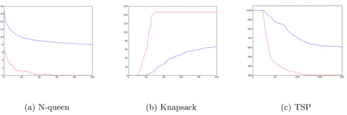
az utazó ügynök, a hátizsák és az N-királynő probléma esetében is megmutattam, hogy (bizonyos paraméterek esetében) a lokális mintavételezéssel gyorsabb konvergencia sebességgel kaphatunk eredményt, mint a globális eljárásnál.
A szimulációkat a gyakorlatban is használt, Xenonv3 architektúrán is implementál- tam, mely kihasználja az általam leírt topografikus módszerek egyik legnagyobb előnyét párhuzamosíthatóságukat és skálázhatóságukat.
A dinamikus probléma esetében Rejtett Markov Modellek állapotbecslését vizsgáltam.
A probléma azért nehéz, mivel nem egy ismeretlen állapotot (optimumot) szeretnék bec- sülni, lehető legjobban megközelíteni, mint a sztochasztikus optimalizációban általában, hanem a markovi modell rejtett állapotait szeretnénk meghatározni, vagyis egy dinamikus, időben változó állapotsorozatot, trajektóriát szeretnék megbecsülni nemlineáris megfi- gyelések alapján. Ezen probléma esetében is három esettanulmányon keresztül mutattam be az eljárás használhatóságát, hatékonyságát. Valamint itt is mind a szimulációs ered- mények, mind a konkrét implementáció a Xenonv3 architektúrán megtalálható.
Dolgozatom második felében spinoszcillátorok szinkronizációjával foglalkoztam, valamint megpróbáltam ezen szinkronizációs jelenségeket a számítási képességek szem- szögéből is megközelíteni. Készítettem egy általános szimulátort mellyel különböző tí- pusú spinoszcillátorok tetszőleges hálózata szimulálható. Analitikus megoldást adtam az
’in-plane’ oszcillációval rendelkező spinoszcillátorok differenciálegyenletének megoldására.
Valamint a harmonic balance és discribing function módszerek alkalmazásával megmutat- tam, hogyan számítható ki egy ilyen elemekből készített tetszőleges hálózatban a külön- böző oszcillátorok közötti fázisszög. Ezáltal egy leképezést adtam, hogy miképpen alakítja át egy STO hálózat a bemenő, frekvencia-kódolt jelet a kimeneti, fáziskódolt jellé. Továbbá megmutattam,hogy ezen fázisszög, hogyan függ a csatolás erősségétől és a bemenő áramtól két oszcillátor esetén.
6
Abstract
In this thesis I would like to examine how local topographic algorithms can be imple- mented and used in practical problems. Nowadays in engineering one of the most chal- lenging task is the design of topographic algorithms that can be executed on topographic architectures.
As we have seen in the previous years the speed of Moore’s law is further decreasing and the operating speed of processor has not increased significantly either. However the number of transistors that can be manufactured on a silicon wafer is increasing further and further. This creates a gap between high level/abstract algorithms and the many-core architectures. We can not yield for higher processing speed has decreased but we can have more parallel cores instead. Because of this phenomena in parallel algorithms on many-core architectures the wire delay became the most determining factor instead of the gate delay.
The transfer of data between the cores can decrease the execution speed significantly. To avoid this we have to process all the data locally, and avoid global communication as much as possible. The only communication which is affordable in a fast, efficient way is the local topographic data exchange.
It is extremely complicated and difficult to examine all the algorithms from this point of view. The general theoretical investigation how general algorithms can be implemented on many-core architectures is out of the scope of this dissertation. Because of the theoretical complexity of many-core implementations I have selected only one type of algorithm:
selection mechanism in stochastic processes and examined how they can be implemented in an efficient topographic way.
There are numerous different algorithms amongst the processes used in stochastic optimization. I also have to note that sometimes not only the problem representation, but also the algorithm itself depends on the problem (especially in case of different heuristic improvements). But we can also see, that in almost every stochastic optimization tasks there are common steps.
I have tried to see and describe these algorithms from a point of view which is rela- tively independent from the problems itself. One of the key steps in this processes is the selection step, when we have to generate a new sample from our current population. I have introduced and examined the biologically inspired selection, and compared these methods (in case of some problems) to some other algorithms containing global selection.
7
I have tried to start these comparisons from a meta-level, where the program repre- sentation is not important, to show that the selection has the same properties in general.
I have shown that in general the local selection can be considered as a generalized ver- sion of the global selection. I have zoomed from this general problem to the more specific problems, to show, that these can be used also not only in theory but also in practical problems.
Later I will show two sample algorithms (widely used in practical problems, which are originally non-topographic) in which case the topographic, cellular way of thinking works better, than the general methods. I will also try to underline this theory by different simulations.
These simulations were implemented on a virtual many core architecture.
The static algorithm (the genetic algorithm) was tested on three different problems on the knapsack, N-queen and on the travelling salesman problem.
I have tested my version of the algorithm not only by simulations but I have also implemented them on an existing chip on the Xenonv3 architecture, which exploits the main characteristics of modern architectures namely the parallel procession, many core execution, scalability and local, cellular connections between the cores.
In case of the dynamic version of the algorithm I describe how the topographic method can be used for state estimation in case of Hidden Markov Models. This problem is more complex than the previously described optimization, because our aim is not to find the best parameters with numerous number of iterations, but to find a hidden state in every iteration, to identify a trajectory of a process. This means that we have only a limited number of steps for processing (usually only one) to identify a dynamically changing state.
Also in this case I have shown through three case studies how this algorithm can be implemented and used, and I have also examined the efficiency of the implementations.
Also in this case I have examined the efficiency based on the simulations with the virtual cellular machine, and also on the existing architecture, theXenonv3 chip.
In the second part of my thesis I have examined how a cellular architecture can be realized by spin torque oscillators. In this architecture all the computation is performed by the physics of the oscillators and the interactions between the neighboring oscillators.
Other different interactions are unfeasible, because of the underlying physics. The results a cellular architecture. I have investigated the synchronization of these oscillators, and how they can be used for computation, where the information is not the charge (as it is in the devices used nowadays), but the phase-shift between the neighboring, synchronized oscillators. This results a non boolean, nanoscale device.
In the second part of this thesis I will show an architecture, which is inherently to- pographic. This processor is made of Spin torque oscillators. The information exchange, interaction between these oscillators happens through the magnetic field. Because of this interaction only a cellular locally connected architecture is feasible.
To implement a processor we can not avoid to understand the behavior of spin torque 8
oscillators. In the second part of this thesis I will describe how we can understand and simplify the synchronization of weakly coupled oscillator networks.
I have implemented a simulator in C, Python and Matlab. With this program I man- aged to investigate the behavior of the STO arrays in general. I have also calculated the equilibrium of an STO with a closed formula and this way the behavior can be calculated, without solving the differential equations.
Using the harmonic balance and the describing function technique I have shown, how the behavior of the synchronized oscillation can be calculated in any arbitrary array. Apart form the transient behavior, any phase shift, frequency and spin position can be examined in any arbitrary array regardless the boundary condition, initial condition, or coupling weights between the elements in the array.
I have also investigated more detailedly the case of two coupled oscillators. I have calculated how the phase shift between the two synchronized oscillator depends on the input current on the oscillators and on the coupling weight between the oscillators.
9
Contents
1 Introduction 14
2 Local and Global Selection Mechanism 16
2.1 Random Sampling and Locality in Stochastic Optimization . . . 16
2.2 General Model of Stochastic Selection . . . 20
2.2.1 The Model . . . 20
2.2.2 Results . . . 21
2.3 A More Specific Model . . . 24
2.3.1 Model . . . 24
2.3.2 Results . . . 26
3 The Application of Stochastic Local Search in Practical Problems 29 3.1 Genetic Algorithms . . . 29
3.1.1 The Nonparalellized Genetic Algorithm . . . 30
3.1.2 Cellular Version of the Genetic Algorithm . . . 33
3.1.3 Three Practical Test Cases . . . 33
3.1.4 Simulation Results on a Virtual Cellular Machine . . . 38
3.1.5 Implementation on the Xenon Architecture . . . 40
3.1.6 Performance Analysis . . . 46
3.2 The Applicability of Local Selection in cGAs on Multiparallel Architectures 48 4 State Estimation of Hidden Markov Models 50 4.1 Filtering, Smoothing, Prediction . . . 51
4.1.1 The General Case . . . 51
4.2 Dynamical Optimization - Particle Filtering . . . 52
4.2.1 Hidden Markov Model and Particle Filtering . . . 53
4.3 Cellular Particle Filter . . . 54
4.3.1 Resampling (step 2) in the cellular particle filter . . . 55
5 Application of the Cellular Particle Filter 57 5.1 Models . . . 57
5.2 Results . . . 59 10
5.3 Setting the Speed of Information Propagation . . . 62
5.4 Diversity of the particles - The Reason for a Lower Error Rate . . . 64
5.5 Another Possible Solution to Improve Information Propagation . . . 67
5.6 Distribution of the Particles . . . 68
5.7 The Applicability of Cellular Particle Filter in Practical Problems . . . 70
6 Dynamics of Spin Torque Oscillators 72 6.1 Spin Torque nano-Oscillator . . . 72
6.2 Spin Torque nano-Oscillator arrays . . . 75
7 The phase equation of Synchronized network of Spin oscillators 77 7.0.1 Dynamical properties of STO . . . 77
7.0.2 Frequency and amplitude of the oscillation . . . 79
7.1 Spin Torque nano-Oscillator arrays . . . 80
7.1.1 Cellular STO arrays with interactions in Mz(t) only . . . 82
7.1.2 Cellular STO arrays with general interactions . . . 83
7.2 When rx equals ry . . . 85
7.3 Two coupled oscillator . . . 87
7.3.1 Coupling only in the Mz component . . . 87
7.3.2 General coupling of two Oscillators . . . 88
7.4 Applications of spin torque oscillators . . . 91
7.4.1 Application example: edge detection . . . 91
7.4.2 Application example: spatial change detection . . . 92
8 Summary 94 8.1 Methods used in the experiments . . . 94
8.2 New scientific results . . . 95
8.3 Application of the results . . . 100
9 Conclusion 102 10 Appendix 104 Appendix ACNN summary . . . 104
Appendix BXenon Architecture . . . 107
Appendix CGenetic Algorithm . . . 111
Appendix DParticle Filter . . . 115
11
List of Figures
2.1 Spatial distribution of the processors, the CNN architecture . . . 19
2.2 Comparison of the local and global selection . . . 27
3.1 Results of the cellular genetic algorithm . . . 41
3.2 The schematic architecture of theXenon_v3 chip . . . 42
3.3 The implementation of the steps of the cellular genetic algorithm on the different layers of a CNN-UM . . . 43
5.1 An example demonstrating the the accuracy of the cellular particle filter . . 64
5.2 The number of ’good’ particles for a sample trajectory . . . 65
5.3 The number of different particles for a sample trajectory . . . 66
6.1 Schematic of a spin device, electrons are spin polarized . . . 73
6.2 Oscillation of two STOs . . . 75
7.1 The evolution of theMz(t) component of two STOs . . . 78
7.2 The magnetization precession vector M(t) of two two STOs . . . . 79
7.3 Limit-cycle of an STO . . . 80
7.4 Phase shifts of synchronized STOs . . . 86
7.5 Oscillation with different coupling strengths inMx andMy components . . 87
7.6 The Mz(t) comoponents of six different STOs . . . 88
7.7 Different limit cycles of diiferent STO arrays . . . 89
7.8 The dependency of the phase-shift based on the current . . . 89
7.9 The dependency of the phase-shift based on the coupling strength . . . 90
7.10 Example of an STO array used for grayscale edge detection . . . 92
7.11 Example of an STO array used for spatial change detection . . . 93
10.1 MxN representation of CNN structure . . . 105
10.2 The output characteristic function of a CNN cell . . . 106
10.3 The architecture of a CNN Universal Machine cell . . . 107
10.4 The schematic architecture of the Xenon_v3 chip . . . 108
10.5 The schematic architecture of a Xenon_v3 core . . . 109
10.6 The structure of the arithmetic unit of a Xenon core . . . 109
10.7 The structure of the morphological unit of a Xenon core . . . 110 12
List of Tables
2.1 Results of the simple model for global selection . . . 22
2.2 Results of the simple model for local selection . . . 23
2.3 Results of the specific model for local and global selection . . . 28
3.1 Average number of iterations for the 16-queen problem . . . 39
3.2 Average number of iterations for the Knapsack problem . . . 39
3.3 Average number of iterations for the traveling salesman problem . . . 40
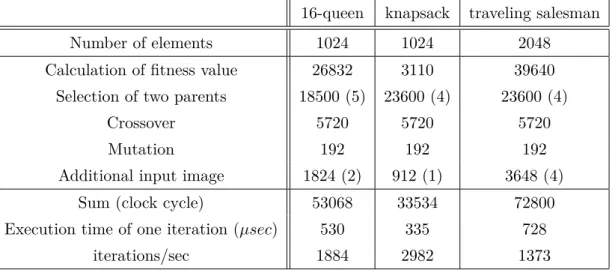
3.4 The distribution of the total running time amongst the operations . . . 46
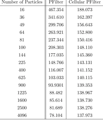
5.1 Results of the first model with different approaches . . . 60
5.2 Results of the second model with different approaches . . . 60
5.3 Result of the three dimensional model with different approaches . . . 61
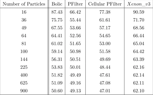
5.4 The running times of different particle filter algorithms on different archi- tectures . . . 61
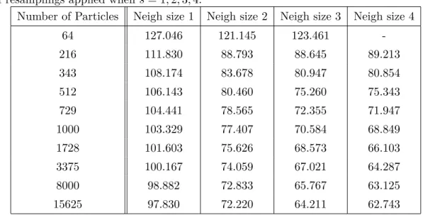
5.5 Results of the three dimensional model with different neighborhood radii using a three dimensional grid . . . 63
5.6 The number total number of particles and the number of different particles close around the estimation for different methods . . . 66
5.7 Result of the three dimensional model with iterative resampling . . . 67
5.8 The distribution of the particles amongst discrete states . . . 70
13
Chapter 1
Introduction
One of the most interesting trend in computer engineering is how multi-parallel ar- chitectures have been brought into focus in the previous decade. Moore’s law – implying that the clock frequency of a processor can be doubled in every second year – is slowing down continuously. Without increasing the clock speed, the obvious method to increase our computational power is to multiply the number of the processing elements. If inventing smarter or faster workers in a task proves to be infeasible, we are still capable of increas- ing the sheer number of workers. Nowadays we are creating architectures specialized for different tasks and further increasing the number of processing elements.
However, to exploit all the advantages of many-core devices it is not enough to use our old algorithms designed for single core chips, we have to change the paradigm of cen- tralized processing. We need new methods and new algorithms. After a certain threshold the number of processing elements may be more than enough, but we still have to divide the work amongst them optimally. The optimization of such a task raises new questions in engineering, new points of view in algorithm design. These designs on many-core archi- tectures underline the precedence of locality. These new topographic, many-core, cellular devices have shown their usability and effectiveness in various tasks. From these solutions we can see, that they can give new, effective solutions in case of topographic tasks (i.e image processing), thanks to the precedence of the locality, and the division of the op- erations based on local communication. Even on the most recent FPGAs data sharing and the communication between the elements could consume more time than the actual
”processing”. Communication considering time and power consumption became one of the main elements of an algorithm. Until this point this question was not investigated in a de- tailed way, although this is one of the most important engineering problem of the following decade.
The most important challenge is not further improving these existing methods on even better architectures 1 , but to identify problem classes, tasks and possibilities when the problems can be transformed into topographic algorithms and mapped on these cellular,
1however this is still a very challenging task of optimization
14
many-core devices.
Unfortunately, the question of how to implement a proper algorithm on a many core architecture is too general and can not be answered. In this dissertation I will investigate a set of algorithms, Sequential Monte Carlo methods, and especially one, very important step of such processes the stochastic local selection of elements. I will show the effectiveness of randomly selected local elements and how they can affect the algorithms. I will investigate this selection independently from the problem representations and compare the selected sets with local and global selection regardless of the problems. I will do this through a general, simplified model, which is based only on the local selection of elements. With this model I will show that the local selection can be considered as a generalized version of the global selection and also a generalization of those methods where there is no selection at all.
Later in this dissertation I will show a few examples and algorithms how the local selection can be used on many-core chips. I will investigate the problem also in case of a dynamic environment, where the optimal state changes in time 2. I will show, how this idea can be used in case of genetic algorithms and in particle filters.
With the genetic algorithm I will investigate three practical problems: the knapsack, N-queen and the travelling salesman problem. I will investigate the particle filter problem through commonly used benchmark models with one and three dimensional state spaces.
According to our current knowledge in physics after a certain point Moore’s law and the downscaling of processors have to stop and they are hindered by the physical constraints in the atomic scale. It is unfeasible to build transistors using only a few atoms. In the second part of this dissertation I will investigate one possible architecture, considering in general what main criteria we have to fulfill beyond Moore’s law and how a functioning device can be implemented, where the processing elements are single atoms. I will give an example of this device: an array of weakly coupled spin-torque oscillators and I will show some examples of the capabilities of this network.
All the mentioned algorithms, figures and also a digital version of this document can be found on the attached CD.
2state estimation of dynamic processes
15
Chapter 2
Local and Global Selection Mechanism
2.1 Random Sampling and Locality in Stochastic Optimiza- tion
It is an interesting phenomenon, how limitless the freedom of thinking is. Maybe this could be the biggest advantage and present of our life, that our imagination allows us to create anything without time, space or any physical constraints. We can not feel the difference between imagining 10 or one billion state variables.
However, when we have to implement an algorithm we have to obey physical rules, constraints, because the functionality of our device is inherently bounded in time and space. With only one processing unit we only have to solve the problem of time, the space itself is not important1.
In contrast, on a many-core architecture, even unwillingly, we have to consider how the processing units are placed and connected. We have to consider the well-defined place of implementation, we have to map our method onto a two dimensional wafer2 and this implies the precedence of locality and in the end – even if we have not considered this before – our algorithm will be topographic, because it is bounded in a two dimensional state space, where only local connections are allowed and efficient. 3
We can also observe locality and physical rules in nature. Every living creature is bounded to its territory and they apply inherently the precedence of locality. We can see that, in case of evolution, the improving of different generations depends on space, different entities at different places found different obstacles to overcome and find different mates to create new entities and generations. However, in most cases 4 the population itself is
1the placement of one element is indifferent
2We are not considering vertical integration for simplicity
3global connections are feasible as series of local connections
4not considering islands or physically separated animals, which would lead to island model genetic algorithms (see [11])
16
global. During the evolution of populations the information 5 can spread out to every individual, but the selection and the comparison of the entities happens always locally.
This is quite similar to our architecture regarding that they are both bounded in space.
It is an interesting task in biology to compare two different species with different mating customs, whether salmons or catfishes 6 have a better and more resistant gene-pool for environmental changes. These are the main idea, why I have decided to investigate local stochastic selection on many-core architectures.
One of the most commonly used operations in stochastic optimization is the selection of a set of elements from our observed data that will 7 represent and preserve correctly some important properties of the full cohort. This operation is a key step in almost every stochastic algorithm that determines the set of elements our process will work with.
This sampling is random, because our models, observations, or our estimations are stochastic. It is important to decide how we can select the best elements randomly from a general set to ensure that the distribution of this element would be the ’best’ for us in some sense. Of course the definition of the ’best set’ itself is especially difficult and a very interesting question, however, it is impossible to investigate this question in full depth in the present work.
This question will be even more interesting when it is applied to many-core architec- tures, namely: how we can select the best set, meanwhile we would like to distribute our effort amongst many elements uniformly. This problem is interesting in theory, but since many-core architectures 8 have been brought to focus in the previous decade it has also a large impact on the efficient solution of practical problems.
The problem in this form itself is too general and can not be investigated, because the algorithm 9 depends on the problem representation and on the problem itself. For this reason I have decided to avoid specifying the problem in this chapter and I will rather create a general model that considers only the main, crucial steps of the algorithm and those principles that are common in every solution, but also specific enough to contain random set of elements and the selection of entities based on certain principles.
The idea of local selection itself was motivated by biological selection. I also wanted to investigate, how biologically inspired computing 10 can help us in case of stochastic optimization.
In many areas and applications we can witness how biology inspired algorithmic prin- ciples can outperform other rivals. We can also see the wonders of biology: how mammals and insects can solve difficult tasks in a simply brilliant way, that can not be solved by
5in this case a good genome or gene
6Salmons mate at the same place every year and the population gathers globally, meanwhile catfishes select mating partners in their territory
7hopefully and according some heuristics or a priori information
8FPGAs, GPUs, CNNs
9or the optimized version of the algorithm
10the local selection and evolution of individuals
17
thousands of engineers. In this section I would like to show how a simple example, what can be observed in real life: evolution can inspire us during algorithm development (especially in case of stochastic optimization) to build proper methods for many-core architectures.
In the literature we can find many articles examining the properties of global and local selection from different aspects, however, these questions are raised by biologists and philosophers, see [12].11. In those papers where we can identify the aspect of engineering points of view, usually well specified, but special problems are examined based on this idea ([13], [14]) or sometimes some small classes or subsets of problems [15] without considering generalization or architectural planning or implementations.
Since the literature of this area is not comprehensive and the published papers are focusing on well-specified problems and not on algorithmic principles I have tried to find a general framework of the problem. Going against the tendencies I have not selected a specified problem to try to make general conclusions later on but I have tried to create a general model of the problem, to formulate general statements and later on I have tried to specialize, narrow down this model to practical problems without changing the main steps of the algorithm. Keeping the algorithm in focus during the whole time and handling the problem itself only as a tool, which is necessary to test our algorithm.
From an engineering point of view this comparison raises many questions. Which method is more effective? In what sense can we measure efficiency? Which method is faster, considering the number of iterations, or considering milliseconds? How we can di- vide the processing optimally amongst the processing units? Is it better to handle all entities of our sample together and we are creating a global order or applying a limit for every processing unit we store only a subset of the sample, and only local interactions are possible between the elements?
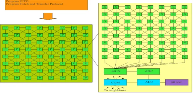
To investigate local constraints I have placed our processing elements in a homoge- neous, rectangular grid. 12. The structure of this grid can be seen on Fig. 2.1, which is the same as the structure of a CNN: a cellular network. A detailed description of the CNN architecture can be found in Appendix A. According to our hopes it can be easily seen that this can be mapped in a straightforward way on any multi-core system, like the Xenon_v3 or an FPGA. A detailed desription of the Xenon architecture can be found at Appendix B.
On first read one could think, that the local selection is much simpler13, than the global process, because we do not have to compare all the elements with each other and we do not have to order all the elements. Although this is true, because we will order only smaller sets in the population, and this will decrease the running speed. However, the algorithm will be more complex: we will have an extra parameter, the just introduced locality, the
11These point of views are not better or worse, but regarding engineering aspects can not be compared or used for algorithm development
12other grids with hexagonal or triangular positions could also be used, and especially heterogeneous grids can create interesting behaviors [11]
13in implementation and also in efficiency
18
Figure 2.1: On this figure we can see the spatial distribution of the processors and also the interconnection between them. The locality in this case is defined by a neighborhood radius r = 1, which means the neighbors are those cells, which are closer than one unit.
This neighborhood will define the communication between the elements and also how the information is divided and spreads out through the network.
size of the smaller sets. Although it is true, that this will result a more complex algorithm, and the theoretical investigation will be more difficult, but with this new parameter we did not create something totally new and different. We have only widened the possibility and the level of adaptation in our algorithm. If we set the neighborhood radius to a relatively large number 14 , then we will get back our global method, when all the elements are compared to each other and there is an interaction between any selected two elements.
Also, if we set the neighborhood radius to zero15, there will be no information exchange between the processing units, and we will get back the result when there is no selection at all. These two extreme situations are interesting and used in practice, however for us (from an engineering point of view) it is more challenging to examine with simulations the case when the neighborhood radius is between these two extrema and to see how information exchange can modify the local selection and the result of our algorithm.
Because the theoretical investigation of a general algorithm is problematic, I have de- cided to create experiments with a general model about stochastic selection. My aim was to create a framework that mimics all the properties of stochastic selection regarding prac- tical problems, however it is general and in this sense independent from the representation of the problem itself.
14larger than the maximal distance between any two elements in the grid
15we will deny all interactions
19
2.2 General Model of Stochastic Selection
2.2.1 The Model
In this subsection I will describe a simple model that grasps the essence of stochastic selection, without being to specific to have any connections with practical problems. I will start my investigation with this model and later on I will specify this general model, to show that it has a strong relation and can be applied in case of practical problems.
Examining stochastic selection and local searches in general we can identify that all these algorithms have the following common steps:
In the beginning of the process a sufficiently large amount of random samples was cre- ated by our previously given distribution. This distribution, if we do not use any problem specific heuristics, is usually uniform or normal and covers the state space. I have to note that the initial distribution should not play a crucial role in the algorithm, because the convergence of the algorithm should hold for an arbitrary -random- initial population.
We have an initial sample (sometimes called population) generated by normal distri- bution in the N dimensional state space 16. We have to evaluate this initial population based on the fitness of every element. The fitness function is a scalar function, that maps the elements of the population to real numbers.
To avoid the over-representation of certain elements in the population, we will alter all the weights randomly. Later on we will recombine elements of the population and mutate them. This means, that based on a randomly driven function we will alter them (move, perturb them in the state space). This perturbation is made by a deterministicφfunction, that maps state x, the state we would like to optimize and by random processes (γt.i), which is the stochastic part of the optimization.17
wt,i=φ(xt,i) +γt,i (2.1)
This weight, generated by the fitness function is the only element 18 that affect the selected elements. To get rid of the problem representation, we will ignore everything in the population, except these weights (w) in what follows.
w0,i ∼N(0, σ1), i= 1. . . K (2.2) In the beginning we will create thisK elements from independent samples. Intuitively we have to preserve the best elements in the population. To preserve these elements we have to create the next population randomly based on nothing but the fitness value of the elements. This will ensure, that the elements with higher fitness will have a larger chance to be a part of the next generation. This is called the selection step. However I also have to
16whereN is the dimension of the problem
17here I use an additive noise, but this is not necessary
18apart from random Independent Identically Distributed (IID) variables
20
note, that the best population is not necessarily a population containing only the clones of the best element, “diversity” of the population may also be desirable. We will investigate this problem later.
Here we have reached again the surface of the problem representation. We can see that this equation contains the state x again. To avoid the problem representation, we have to get rid of x. During the selection the state is not important for us, only the weight w itself. This is the other simplification of this general model. Lets assume, that this operation changes the weight by a normal additive noise.19This approximation that these operations are represented as an additive normal noise can be justified: large changes happening with low probability, and usually only small changes will occur during the mutation step. Also if the change is stochastic, we can assume that a random change in the genome will as likely increase its fitness as decrease it. This way we can concentrate only on the scalar weight function:
wt+1,i=wt,i+ξt,i (2.3)
Where ξt,i ∼N(0, σ2) are independent. We can try to investigate the performance of local search based on this simple, general model and compare global and local selection.
As we can see from this state transition it can happen that during the algorithm we will generate elements with negative weights (this problem can be avoided problem easily, because one could compare the relation of the weights instead of the direct weight or add a large sufficiently large constant to every weights). I chose zero as a minimal weight and I set all the negative values to zero before every selection step.
2.2.2 Results
The parameters of the model applied were the following: σ1 = 10, σ2 = 3
To compare the global and local selection mechanism I have generated a sample with K = 400 elements and these elements were placed on a 20×20 two-dimensional grid in case of the local sampling. In every experiments I examined the 10th population20 and I have repeated every experiment 1000 time to reduce the noise of the simulations caused by the stochastic nature of the processes.
After the 10th iteration I have selected the best element 21. The results of the global selection as the average of 1000 simulations can be seen in Table 2.1
While in case of global selection the number of selected parameters were determined directly by one, and only one parameter. In case of local selection we can set the neighbor- hood radius, in which distance we will examine the elements in a region of a cell. Even if it is not clear for the first read this is very similar to the parameter of the global selection.
19this is a generalization, but during stochastic optimization we generally use small perturbations in the state space. The effect of this small perturbation can be assumed to be normal additive noise
20the population after 10 selection and mutation steps
21the element with the highest fitness weight
21
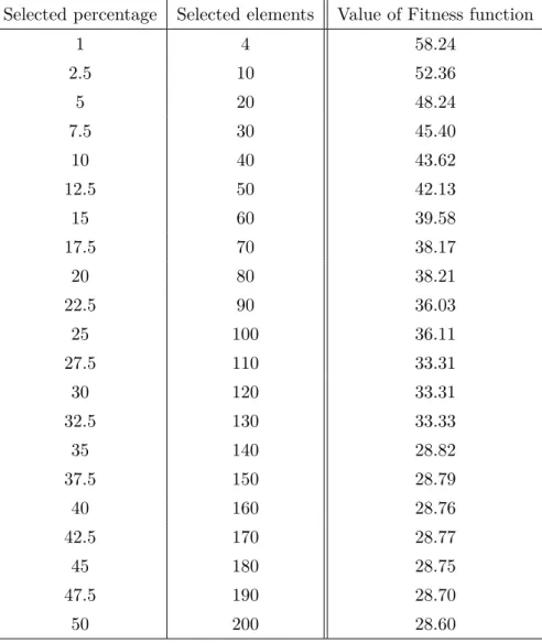
Table 2.1: Results of the simple model for global selection
The first column shows the amount of preserved elements during the selection step in percentage, The second column shows how many elements were selected during the se- lection step. The last column shows the highest value of the fitness function w obtained by this parameters. The fitness values were calculated as the average of 1000 independent simulations, the higher values mean better results.
Selected percentage Selected elements Value of Fitness function
1 4 58.24
2.5 10 52.36
5 20 48.24
7.5 30 45.40
10 40 43.62
12.5 50 42.13
15 60 39.58
17.5 70 38.17
20 80 38.21
22.5 90 36.03
25 100 36.11
27.5 110 33.31
30 120 33.31
32.5 130 33.33
35 140 28.82
37.5 150 28.79
40 160 28.76
42.5 170 28.77
45 180 28.75
47.5 190 28.70
50 200 28.60
22
Previously I have described, how we can derive the global selection from the local version.
If we observe this phenomena from an other point of view, it is even easier to realize the similarity. Lets imagine that we have one extremely good element in our population, with a very high weight . In the next step this element will be copied, cloned to the cells within the previously given neighborhood radiusr. This parameterrwill determine, how cells will see a good element: how visible it is and how it will be represented in the population. This means an upper bound, how many times the best element can be copied in one iteration, and in this sense this is very similar to the percentage of selected and preserved elements in case of the global mechanism.22
The result of the local selection mechanism can be seen in Table 2.2.
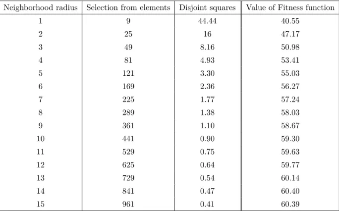
Table 2.2: Results of the simple model for local selection
The first column of the table contains the neighborhood radiusr. The second column show how many elements are in a set defined byr. The third column is to help expressing the connection between the local and global selection mechanisms. This value can be calculated fromrand represents the number of disjoint squares that can be placed on the grid used in the simulations. This means that in one step we will have at least this many independent selections for the middle element of these squares. The last column shows the value of the Fitness function (w, taken from 1000 independent simulations).
Neighborhood radius Selection from elements Disjoint squares Value of Fitness function
1 9 44.44 40.55
2 25 16 47.17
3 49 8.16 50.98
4 81 4.93 53.41
5 121 3.30 55.03
6 169 2.36 56.27
7 225 1.77 57.24
8 289 1.38 58.03
9 361 1.10 58.67
10 441 0.90 59.30
11 529 0.75 59.63
12 625 0.64 59.77
13 729 0.54 60.14
14 841 0.47 60.40
15 961 0.41 60.39
As it can be seen from the comparison of the results, the general model of stochastic sampling with local sampling gives approximately the same results (for some parameters
22Of course we have to note, that the neighborhood radius will not only affect this property, it will also increase the section of elements seen by two cells in proximity.
23
even better) than the global selection. in case of neighborhood radius 9, the maximal fitness value will be 58.67, we will have a similar value (58.24) with the global sampling when we select only the best 4 elements in every population of 400 entities. When we set the neighborhood radius to 123, the fitness function will be 40.55, which is relatively high comparing the two different methods.24
Based on this results we can think, that the local selection can substitute its global counterpart, and the global algorithm is easily parallelizable and scalable and can be mapped easily to many-core architectures. Meanwhile collecting and comparing all the elements we would loose the biggest advantage of today’s architectures: parallelism.
I have to mention, that in case of stochastic optimization our goal is dual. On one hand we would like to maximize the fitness value (we have investigated this scenario), on the other hand we would like to achieve the most diverse population possible, to avoid the local extrema in the state space and mutate our entities towards the global extremum.
Based on these properties I can state, that in case of the global selection, when we preserved only the best 4 elements (58.24 fitness value) the diversity of the population will be much lower than in case of the local selection. We can approximate this amount based on the lower bound on this property in table 2.2. As we will see it later the actual diversity is much larger. This would cause, that in case of a practical problem with many local extrema the global selection mechanism would perform more poorly than its local counterpart.
In this model local extrema do not occur, so the algorithm, in a sense, is trivial. For this reason we consider a slightly more complex model in the next section.
However, this can not be examined by this simple model, because it is too general and we can not add local extrema in it. Hence the the fitness function is linear.
2.3 A More Specific Model
2.3.1 Model
We have seen in the previous section, that the general model is not capable to reflect one -the biggest and most serious- problem of local stochastic searches: the local extrema.
We have to add this crucial property into our model, without specializing it into practical problems. We have to stay as general as possible. To do this we have to consider the position of the elements in the state space in general, without creating a special state space related to some specific model. To avoid the implementation of a specific state space we can assume that every element in the state space will have a propertyp1, to stuck in a local extremum25and withp0it will not find local bounds around itself in the state-space.
This is of course again a generalization, because in case of a real problem, the state space
23and on every commonly used cellular architecture, this can be done easily
24considering that in case of the global method we would need a large global memory.
25which can be also global extremum
24
is not homogeneous, and elements in different points will have different probabilities to stuck in local extrema. But in this dissertation my scope is not to compare or classify different state spaces, but to compare selection mechanisms, and this model is general but useful enough to reveal one main aspects of local stochastic searches: the diversity of the population. I also have to note that the other operations (recombination, mutation) are the same for both the global and local version of the algorithm, so eventual better results can only be explained by the selection mechanism.
We can also assume that elements close to each other will most likely be altered in the same way: If an element will stuck in a local extremum, we can presume, that all the elements around it will also stuck at the same place in the state space. Also if an element can move/mutate toward a better solution (without getting stuck) all the surrounding elements have the potential to move as well.
To achieve our goal we have to consider somehow the position of the elements in the state space, without specifying the state space itself. If we can label the positions in the state space we can calculate which elements will get stuck together. We also know that when an element with a relatively high weight is selected and copied multiple times there will be more identical elements (at the same position in the stat space) in the next generation before the mutation operator is applied. Based on this I have divided the elements into groups and each group is determined by the identity in the previous generation it was copied from. Thep0 andp1probabilities are applied for every group and they can determine whether a group can mutate (increase the weights of the elements) or not (they stuck in a local extrema)
During the resampling step I divide the elements into groupsαj, j = 1, . . . M according to the previously described rules.Gj-s are binary random (Bernoulli) variables with values zero or one. Withp0 probability αj = 0 and withp1= 1−p0 probability αj = 1.
Then for everyiifwt,i ∈Gj and αj = 0
wt+1,i=wt,i+ηt,i (2.4)
ifwt,i∈Gj andαj = 1
wt+1,i=wt,i (2.5)
Where ηt,i ∼ N(0, σ2) are independent and Gj represents a group of the elements in proximity.
Of course this model is a simplification of the position of the elements in the state space, and I have to note that elements can be in proximity caused by the mutation step as well, not only by the selection mechanism. The elements migrate in the state space and perform stochastic walks and even without a selection mechanism every element should visit all the points of the state space once in a while if the mutation factor is relatively large and we have to note that this model is not considering this temporal ’moving’ of the elements. However in case of a relatively large state space and if the distribution of the
25
elements is uniform in this state space the effect of resampling step driving the elements to the same places is much stronger.
2.3.2 Results
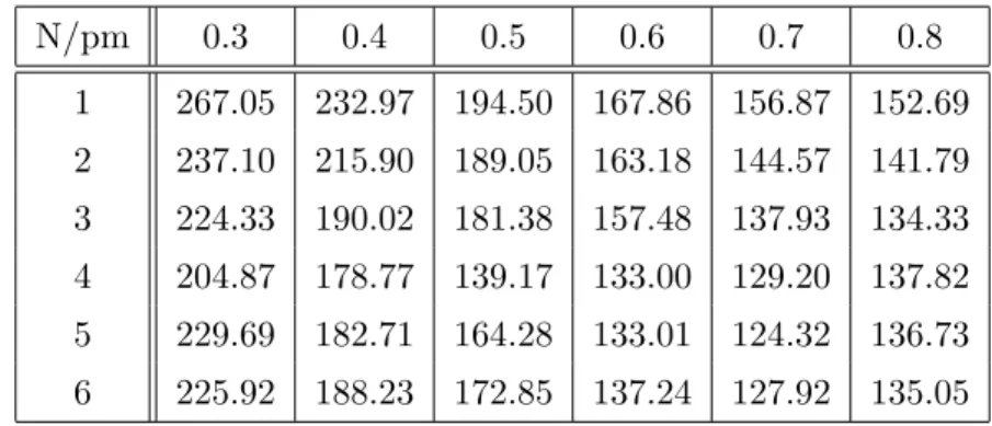
The parameters of the model were:σ1= 10, σ2 = 3,p0= 0.70, p1 = 1−p0 = 0.30 To compare the global and local selection mechanism I have generated a sample with K = 400 elements, and these elements were placed on a 20×20 two-dimensional grid in case of the local sampling. In every experiments I examined the 10th population26 and I have repeated every experiments 1000 time, to reduce the noise on the simulations caused by the stochastic operators.
After the 10th iteration I have selected the best element 27. The results of both the global and local selection as the average of 1000 experiments can be seen in Table 2.3 The graphical interpretation of these results can be seen on figure 2.2.
These result are very important regarding the local selection. This model is the most general, that is capable to represent the most challenging problem of local stochastic optimization. Namely, when we would like to maximize (or minimize) a function we have to have the most diverse set, and cover the whole state space to avoid all the local extrema except the only global extremum.
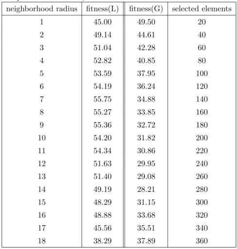
We can derive two conclusions from the results: It can be seen that the local algorithm outperforms its global counterpart. It can also be seen that the values of the fitness of the local selection for different parameters have a concave shape. It is true, that the extreme cases28 are usually not efficient. This implies, that with the proper setting of the neighborhood radius we can optimize the performance of the localized algorithm. We can alter how the information spreads out through the processing elements and this way we can set the exploitation/exploration ratio of the algorithm. This way we can set either our aim is to maximize the fitness function and move towards the best value (case of global interactions) or to maintain the most diverse population possible (no interaction at all).
In case of a specific problem we can set the best parameter considering the probability of finding a local extrema. Setting this parameter to an optimal value we can solve practical problems more easily and efficiently. Because this dissertation investigates primarily the implementation and design of many-core algorithms, I stress the importance of the fact, that the local selection mechanism can be easily parallelized and its execution time can be decreased to a fraction of the execution time of the global method.
26the population after 10 selection and mutation steps
27the element with the highest fitness weight
28small local interactions or large ,global interactions affecting the whole population
26
Figure 2.2: On this figure we can see the results of the local (red, continuous) and global selection (blue, dashed) mechanism. The numbers on the X-axis are the parameters, in every bracket the first is the neighborhood radius for the local method and the other is the number of the selected elements for the global method. The experiments were done withK = 400 elements. On the Y-axis we can see the fitness values, higher values mean better solutions. It can also be seen that the values of the fitness of the local selection for different parameters have a concave shape. This implies, that with the proper setting of the neighborhood radius we can optimize the performance of our algorithm by picking out the parameter value corresponding to the tip of this curve.
27
Table 2.3: Results of the specific model for local and global selection
The first column of the table shows the neighborhood radius for local selection r. The second column is the result of the local method , the maximal value of the fitness function w (as an average of 1000 independent simulations). The third column is the result of the global method The last column represents the parameter of the global selection, the number of selected elements. As it can be seen the best result can be obtained with the local method, however the comparison of the two methods for one parameter-setup is not straightforward, because the parameters in the algorithms (the neighborhood radius and the number of preserved elements) are different.
neighborhood radius fitness(L) fitness(G) selected elements
1 45.00 49.50 20
2 49.14 44.61 40
3 51.04 42.28 60
4 52.82 40.85 80
5 53.59 37.95 100
6 54.19 36.24 120
7 55.75 34.88 140
8 55.27 33.85 160
9 55.36 32.72 180
10 54.20 31.82 200
11 54.34 30.86 220
12 51.63 29.95 240
13 51.40 29.08 260
14 49.19 28.21 280
15 48.29 31.15 300
16 48.88 33.68 320
17 45.56 35.51 340
18 38.29 37.89 360
28
Chapter 3
The Application of Stochastic
Local Search in Practical Problems
Based on the models shown in the previous chapter one can feel that the local stochastic search can be used more efficiently 1 on many-core architectures than its global counter- part. But this reasoning was based only on a theoretical model, which can be too general and could have only a weak link to practical problems. A thorough theoretical investigation can be done only by generalization, however, the problem is too complex to investigate it in the scope of this dissertation. The previous steps were necessary to highlight the utility of the method, but to stress out the application I have to show, that they can be implemented on existing architectures and they can solve existing problems with the same accuracy but with a decreasing running time. It could happen that, because of the gen- erality of the problems, we have forgot some important detail, that can be observed only in case of real problems. I will prove the applicability of the idea of the previous chapter with two commonly investigated and important algorithms.
3.1 Genetic Algorithms
The first practical algorithm that uses the local search is the genetic algorithm and this method is extremely closely related to the previously described models.
Numerous topographic and parallel algorithms have been described in previous years that can exploit the high performance of multi-parallel, Cellular Neural Network (CNN) architecture [1], [2]. These algorithms can be executed with an extraordinary speed; they have been used in image-processing [16], for analyzing three-dimensional surfaces [17], [3], for solving differential equations [18] or for various retina modeling tasks [19].
Genetic algorithms (GA) and their utility in practical problems have been introduced
1Determining the efficiency of an algorithm is an extremely difficult task because one can rank these methods by many metrics: power consumption, running speed,accuracy, prices, area of the implemented chip etc...In this dissertation efficiency is measured as a comparison of execution speed and accuracy on a virtual machine and theXenon_v3 architecture
29
by John H. Holland in 1975, [20]. Since then these methods (with various alterations) have been applied to a large class of problems. These heuristic search algorithms, inspired by natural selection and evolutionary mechanisms, can provide solutions faster than exhaus- tive search, and give better results than greedy algorithms.
It can be observed in biological networks and among organisms that mate selection and genetic inheritance between generations happens locally, according to a topographic rule.
Genomes that are able to overcome the challenges of nature in a well-defined environment (in the territory of the individual) can be inherited to the next generation, and spread out in a diffuse-topographic way in the population.
Examining evolution and natural selection we can see that a parallel and topographic approach is more realistic and similar to the original, motivating idea than the commonly used “global”, non-topographic selection rules. This also refers to GAs, and a parallel topographic implementation can outperform its “regular” single-core ancestors.
Favorable convergence speed of the cellular algorithm has been proved, and the utility of these methods has been demonstrated theoretically in [21], but the ideal implementation on the Cellular Neural Network Universal Machine (CNN-UM)2, has not yet been studied previously.
3.1.1 The Nonparalellized Genetic Algorithm
GAs are stochastic algorithms for search and optimization inspired by natural selection.
A more detailed description of the Genetic Algorithm can be found at Appendix C. Many alterations and changes are known but the following four steps are the fingerprints that determine genetic algorithms and they can be found in all variants and alterations.
• (1) Initialization of the populations
• (2) Fitness (weight) calculation for every genome
• (3) Selection and recombination
• (4) Mutation
Steps 2, 3, 4 are repeated until a previously given time constraint, or until the optimal solution can be found3.
I provide a brief description on these four steps that are relevant to my settings. A more detailed description can be found in [22]
(1) Initialization of the population:
at this step we will create random 4 vectors with values, genomes according to the problem representation.
2which is a true topographic mapping of the algorithm
3when the optimal solution can be identified based on the constraints
4usually uniformly distributed
30
(2) Fitness (weight) calculation:
One has to calculate a fitness, weight value for every genome. This value represents a distance between our solution candidate and an optimal solution in the state space. The metric of the distance is based on problem dependent heuristics. Selecting an appropriate metric is a key question, I base my choice on well-known, published suggestions.
(3/a) Selection of parents:
In case of the panmictic GA, selection is calculated globally, i.e. using all the genomes generated in the previous step. We select the part of the genome we want to conserve and inherit for the next generation, and replace unnecessary elements.
There are many different methods for the selection of the parents because of practical considerations we have selected Stochastic Universal sampling [23]. With this method we need only a relatively low amount of random numbers on the chip 5. The probability of selecting a genome as a parent is proportional to its fitness value. This is one of the most simple step in the algorithm for us and in this selection we can use all the theories and simulation results from the previous chapter, since this is the most similar to stochastic sampling.
(3/b) Recombination:
In this step we will recombine the genes of the selected parents and create a new entity combining their properties. In the first case, we will choose one point in the genome, and until this point all the genes will be inherited from one parent and after this point all the genes will be copied from the other parent. Ideally, the offspring solution obtained through the recombination is not identical to any of the parents, but contains combined building blocks from both.
(4) Mutation:
Mutation performs a random jump in the state space in the neighborhood of a can- didate solution. There exist many mutation variants, which usually affect one or more loci 6 of the individual. The mutation randomly modifies a single solution whereas the recombination acts on two or more parent chromosomes.
The pseudo-code of a GA based on the previous steps can be seen at Algorithm 1.
5which will be a bottleneck of the algorithm as we can see it in section 3.1.5
6genes or components
31
Algorithm 1 Pseudo Code of the Genetic Algorithm using deterministic sampling Pa- rametersP opsSize,M utF act,U sedP op,M axIterare the following:
P opsSize: the size of the population, i.e. the number of genomes used in an iteration.
M utF act: mutation factor. The probability that a randomly selected gene will change its value.
U sedP op: the ratio that determines how many elements will be stored in every iteration, generation. The number of deleted elements is: P opsSize∗(1−U sedP op).
M axIter: the number of maximal iterations. After theM axIter-th iteration the algorithm will stop regardless we have found the optimal solution or not.
Require: M utF act U sedP op P opsSize M axIter Ensure: gmin
gmin⇐1 Iter ⇐0
{/}/1- initialization for i= 0 to P opSizedo
foreverygene ingi do gene⇐randomgene() end for
end for
while Iter < M axIterAND gmin6=F ittnes(optimum) do {/}/2- selection-ordering genes
fori= 0 to P opSizedo Order(gi, F ittnes(gi)) end for
gmin⇐g0
{/}/3-recombination
fori= 0 to P opSize*U sedP op/2 do forj= 0 to P opSize*U sedP opdo gnewj ⇐recombine(gi∗2, gi∗2+1) end for
end for g⇐gnew {/}/4- mutation
fori= 0 to P opSizedo forevery geneingi do
a⇐randomnumber(0,1) if a < M utF actthen
gene⇐randomgene() end if
end for end for
Iter⇐Iter+ 1 end while
32
3.1.2 Cellular Version of the Genetic Algorithm
The panmictic genetic algorithm can not be effectively implemented on a parallel ar- chitecture because for the selection step we need to collect fitness values from all the genomes. All the other steps could be easily implemented on a fine-grained (single instruc- tion multiple data) architecture, where every processing unit represents one genome.
I will use an altered version of GA, a two dimensional variant of the so-called cellular genetic algorithm. The theory of these algorithms was introduced in [24], [25]. Here I will implement a two-dimensional variant on an n×n array, where the radius of the communicating neighborhoods can be set arbitrarily, by repeating the parent selection step with one neighborhood radius. We can set the exploration/exploitation ratio with this parameter, instead of using an n×m grid and varying the n/m ratio, as in [26]. In this method we will determine the parents locally, the selection of the fittest genomes and the recombination is done in a topographic way, just like in the case of real organisms.
In an iteration every genome will select the fittest genomes in a neighborhood of radius N eighSize, and these parents will create the gene pool of the respective genome for the next generation. With this I can ensure parallel execution, and a prefect mapping to a cellular architecture.
In this dissertation I will use only the simplest, but also most general variation of cGA, using single point mutation and single point recombination between two parents and selection based on Stochastic Universal Sampling [23] (This operations are described in Appendix C). This contains all the important features from the implementation point of view. This implementation can be used for solving other types of problems, and can be adapted to improved versions of GAs.
Because heuristic improvements like [27] or [28] nearly always intervene at the stage of mutation, fitness calculation or at other genome-dependent stages they can also be realized in the topographically distributed, multi-parallel implementation on CNN architecture.
After this general description one could easily modify the global algorithm to have the pseudo code of the cGA (the algorithm can be seen at Algorithm 2).
3.1.3 Three Practical Test Cases
For testing the algorithm, I have selected three typical, well documented problems:
theN-queen problem (see [29]) forN = 16,the knapsack problem ([30],[31], [32]) and the travelling salesman problem ([33], [34], [35]).
These are fundamental problems from the field of combinatorial optimization. I have to note that my aim is not to compare the genetic algorithm with other possible solutions but to show the applicability of my implementation.
33