Extending the Rash model to a multiclass parametric network model

(1)

Extending the Rash model to a multiclass parametric network model ^∗

Marianna Bolla

^a

, Ahmed Elbanna

^ab

aInstitute of Mathematics, Budapest University of Technology and Economics

bMTA–BME Stochastics Research Group marib@math.bme.hu,ahmed@math.bme.hu

Abstract

The newly introducedα-β-models and the classical Rash model are united in a semiparametric multiclass graph model. We give a classification of the nodes of an observed network so that the generated subgraphs and bipartite graphs of it obey these models, where their strongly connected parameters give multiscale evaluation of the nodes. This is a heterogeneous version of the stochastic block model, built via mixtures of loglinear models, the parameters of which are estimated by collaborative filtering. In the context of social networks, the clusters can be identified with social groups and the parameters with attitudes of people of one group towards people of the other, which attitudes depend on the cluster memberships. The algorithm is applied to real-word networks.

Keywords:Rasch model, multiclass loglinear models, collaborative filtering MSC:62F86, 05C80

1. Introduction

Recently,α-β-models [1, 2] were developed as the unique graph models where the degree sequence is a sufficient statistic. In the context of network data, a lot of information is contained in the degree sequence, though, perhaps in a more sophisticated way. The vertices may have clusters and their membership may affect their affinity to make ties. We will find groups of the vertices such that the within- and between-cluster edge-probabilities admit certain parametric graph

∗Research supported by the TÁMOP-4.2.2.C-11/1/KONV-2012-0001 project.

Eszterhazy Karoly University of Applied Sciences and Bay Zoltán Nonprofit Ltd. for Applied Research Eger, Hungary, November 5–7, 2014. pp. 15–22

doi: 10.17048/FutureRFID.1.2014.15

15

(2)

models, the parameters of which are highly interlaced. Here the degree sequence is not a sufficient statistic any more, only if it is restricted to the subgraphs. When making inference, we are partly inspired by the stochastic block model, partly by the Rasch model, the rectangular analogue of theα-β models.

We propose a heterogeneous block model by carrying on the Rasch model developed more than 50 years ago for evaluating psychological tests [5]. Given the number of clusters and a classification of the vertices, we will use the Rasch model for the bipartite subgraphs, whereas theα-β models for the subgraphs themselves, and process an iteration (inner cycle) to find the ML estimate of their parameters.

Then, based on the overall likelihood, we find a new classification of the vertices via taking conditional expectation and using the Bayes rule. Eventually, the two steps are alternated, giving the outer cycle of the iteration. Our algorithm fits into the framework of the EM algorithm, the convergence of which is proved in exponential families under very general conditions [4]. This special type of the EM algorithm developed for mixtures is often called collaborative filtering [7].

In the context of social networks, the clusters can be identified with social strata and the parameters with attitudes of people of one group towards people of the other, which attitude is the same for people in the second group, but depends on the individual in the first group. The number of clusters is fixed during the iteration, but an initial number can be obtained by spectral clustering tools. Together with the description of the algorithm and a theorem about the rank of the matrix of logits, the algorithm is applied to real-word networks.

2. The submodels used

Together with the Rasch model, loglinear type models give the foundation of our unweighted graph and bipartite graph models, the building blocks of our EM iteration.

2.1. α-β models for undirected random graphs

With different parameterization, [1] and [2] introduced the following random graph model, where the degree sequence is a sufficient statistic. We have an unweighted, undirected random graph on n vertices without loops, such that edges between distinct vertices come into existence independently, but not with the same probability as in the classical Erdős–Rényi model. This random graph can uniquely be characterized by itsn×nsymmetric adjacency matrixA= (Aij)which has zero diagonal and the entries above the main diagonal are independent Bernoulli random variables whose parameters pij =P(Aij= 1)obey the following rule. Actually, we formulate this rule for the ₁₋^p^ij_p_ij ratios, the so-called odds:

pij

1−pij

=αiαj (1≤i < j≤n), (2.1)

(3)

where the parameters α1, . . . , αn are positive reals. This model is calledαmodel in [2]. With the parameter transformationβi = lnαi (i= 1, . . . n), it is equivalent to theβ model of [1] which applies to the log-odds:

ln pij

1−pij

=βi+βj (1≤i < j≤n) (2.2)

with real parametersβ1, . . . , βn.

We are looking for the ML estimate of the parameter vectorα= (α1, . . . , αn) or β = (β1, . . . , βn) based on the observed unweighted, undirected graph as a statistical sample. (It may seem that we have a one-element sample here, however, there are ⁿ₂

independent random variables, the adjacencies, in the background.) Let D = (D1, . . . , Dn) denote the degree-vector of the above random graph, where Di = Pn

j=1Aij (i = 1, . . . n). The random vector D, as a function of the sample entries Aij’s, is a sufficient statistic for the parameterα, or equivalently, for β, see [2]. Let (aij) be the matrix of the sample realizations (the adjacency entries of the observed graph), di = Pn

j=1aij be the actual degree of vertex i (i= 1, . . . , n)andd= (d1, . . . , dn)be the observed degree-vector. The maximum likelihood estimateαˆ (or equivalently,β) is derived from the fact that, with it, theˆ observed degreedi equals the expected one, that isE(Di) =Pn

i=1pij. Therefore, ˆ

αis the solution of the following system of maximum likelihood equations:

di= Xn

j6=i

αiαj

1 +αiαj

(i= 1, . . . , n). (2.3)

The Erdős–Gallai conditions characterize so-called graphic degree sequences that can be realized as degree sequences of a graph. For given n, the convex hull of all possible graphic degree sequences is a polytope, to be denoted by Dⁿ. Its extreme points are the so-called threshold graphs. The authors of [1, 2] prove that whenever the observed degree sequence is in the interior ofDⁿ, the maximum likelihood equation (2.3) has a unique solution. On the contrary, when the observed degree vector is a boundary point of Dⁿ, there is at least one 0 or 1 probability pij which can be obtained only by a parameter vector such that at least one of the βi’s is not finite.

The authors in [2] recommend the following algorithm and prove that, provided dis an interior point ofDⁿ, the iteration of it converges to the unique solution of the system (2.3). Starting with initial parameter valuesα⁽⁰⁾₁ , . . . , α⁽⁰⁾n and using the observed degree sequenced1, . . . , dn, which is an inner point ofDⁿ, the iteration is as follows:

α^(t)_i = di

P

j6=i 1

1 α(t−1)

j

+α^(t−1)_i

(i= 1, . . . , n) (2.4)

fort= 1,2, . . ., until convergence.

(4)

2.2. β-γ model for bipartite graphs

This bipartite graph model traces back to Rasch [5], who investigated binary tables.

Given anm×nrandom binary arrayA= (Aij), or equivalently, a bipartite graph, and using the notationpij=P(Aij = 1), our model is

ln pij

1−pij

=βi+γj (i= 1, . . . , m, j= 1, . . . , n) (2.5)

with real parameters β1, . . . , βm and γ1, . . . , γn. In terms of the transformed pa- rametersbi=e^βⁱ and gj=e^γ^j, it is equivalent to

pij

1−pij =bigj (i= 1, . . . , m, j= 1, . . . , n) (2.6) where b1, . . . , bm andg1, . . . , gn are positive reals. Observe that these parameters are arbitrary to within a multiplicative constant.

Here the row-sums Ri = Pn

j=1Aij and the column-sums Cj =Pm

i=1Aij are the sufficient statistics for the parameters collected in b = (b1, . . . , bm) and g = (g1, . . . , gn). Based on an observed binary table(aij), since we are in exponential family, and β1, . . . , βm, γ1, . . . , γn are natural parameters, the likelihood equation is obtained by making the expectation of the sufficient statistic equal to its sample value. Therefore, with the notationri=Pn

j=1aij(i= 1, . . . , m)andcj=Pm i=1aij

(j= 1, . . . , n), the following system of likelihood equations is yielded:

ri= Xn

j=1

bigj

1 +bigj

=bi

Xn

j=1

1

1 gj +bi

, i= 1, . . . m;

cj = Xm

i=1

bigj

1 +bigj

=gj

Xm

i=1

1

1 bi +gj

, j = 1, . . . n.

(2.7)

Note that for any sample realization ofA,Pm

i=1ri=Pn

j=1cj holds automatically.

Therefore, there is a dependence between the equations of the system (2.7), indi- cating that the solution is not unique, in accord with our previous remark about the arbitrary scaling factor.

Like the graphic sequences, here we define so-called bipartite realizable sequences, the convex hull of which is the polytopeP^m,n. In [6] it is proved that the maximum likelihood estimate of the parameters of model (2.6) exists if and only if the observed row- and column-sum sequences are in the relative interior of P^m,n. Under these conditions, we define an algorithm that converges to the unique (up to the scaling factor) solution of the maximum likelihood equation (2.7). Starting with positive parameter valuesb⁽⁰⁾_i (i= 1, . . . , m)andg_j⁽⁰⁾(j= 1, . . . , n)and using

(5)

the observed row- and column-sums, the iteration is as follows:

b^(t)_i = ri

Pn

j=1 1

1 g(t−1)

j

+b^(t−1)_i

, i= 1, . . . m

g_j^(t)= cj

Pm

i=1 1

1 b(t)

i

+g^(t_j⁻¹⁾

, j= 1, . . . n

for t = 1,2, . . ., until convergence. Convergence facts are obtained by the weak contraction property of the transformations yielding the sequence of the iteration.

3. The multipartite graph model

In the several clusters case, the above discussed submodels are the building blocks of a heterogeneous block model. Here the degree sequences are not any more sufficient for the whole graph, only for the building blocks of the subgraphs.

Given 1 ≤ k ≤ n, we are looking for k-partition, in other words, clusters C1, . . . , Ck of the vertices such that different vertices are independently assigned to the clusters and, given the cluster memberships, verticesi∈Cu andj∈Cv are connected independently, with probabilitypij such that

ln pij

1−pij

=βiv+βju, (3.1)

for any1≤u, v≤kpair. Equivalently, pij

1−pij

=bicjbjci,

whereci is the cluster membership of vertexi andbiv =e^β^iv.

The parameters are collected in then×k matrixB of biv’s fori ∈Cu u, v = 1, . . . , k, and are estimated via the EM algorithm for mixtures (collaborative filtering). HereA= (aij)is the incomplete data specification as the cluster memberships are missing. First we complete our data matrixAwith latent membership vectors m1, . . . ,mn of the vertices that arek-dimensional i.i.d. multinomially distributed random vectors. More precisely,mi= (mi1, . . . , mik), wheremiu= 1ifi∈Cu and zero otherwise.

Starting with initial parameter valuesB⁽⁰⁾ and membership vectors m⁽⁰⁾₁ , . . . ,m⁽⁰⁾n , thet-th step of the iteration is the following (t= 1,2, . . .).

• E-step: we calculate the conditional expectation of each mi conditioned on the model parameters and on the other cluster assignments obtained in step t−1, via taking conditional expectation (in the possession of binary variables, the Bayes rule is applicable).

(6)

• M-step: We estimate the parameters in the actual clustering of the vertices.

In the within-cluster scenario, we use the parameter estimation of model (2.1), obtaining estimates ofbiu’s (i∈Cu) in each cluster separately(u= 1, . . . , k);

herebiucorresponds toαiand the number of vertices is|Cu|. In the between- cluster scenario, we use the bipartite graph model (2.6) in the following way.

Foru 6=v, edges connecting vertices of Cu and Cv form a bipartite graph, based on which the parametersbiv (i∈Cu) andbju(j ∈Cv)are estimated with the above algorithm; herebiv’s correspond to bi’s, bju’s correspond to gj’s, and the number of rows and columns of the rectangular array corresponding to this bipartite subgraph ofAis|Cu|and|Cv|, respectively. With the estimated parameters, collected in then×k matrixB^(t), we go back to the E-step, etc.

By the general theory of the EM algorithm, since we are in exponential family, the iteration will converge. Note that here the parameter βiv with ci = uembodies the affinity of vertex i of cluster Cu towards vertices of cluster Cv; and likewise, βjuwith cj =v embodies the affinity of vertexj of clusterCv towards vertices of cluster Cu. For selecting the initial number of clusters we used spectral clustering tools.

Theorem 3.1. Let the n×n symmetric matrix L contain the log-odds satisfying the model equation (3.1) as its entries. Then rankL≤2k.

Proof. LetBe denote then×kmatrix ofβiv’s fori∈Cu,u, v= 1, . . . , k. We define the n×n matrixU as follows: uij :=βicj (i, j = 1, . . . , n). Then L=U+U^T. This is obvious if we understand the structure of the matrixU; actually, it is the one-sided blow-up of the matrixBe as the columnsj1 andj2ofUcontain the same entries whenevercj1 =cj2. Therefore, there arek different types of columns ofU, as many as the number of the clusters, and the columns occur with multiplicities nv = |Cv| (v = 1, . . . , k). Consequently, rank(U) = rank(U^T) ≤ k, and, by applying rank theorems, rankL=rank(U+U^T)≤2kthat finishes the proof.

Remark 3.2. Let U = Pk

l=1slxly^T_l be SVD, where s1 ≥ · · · ≥ sk are the non- zero singular values of U with unit-norm singular vector pairs xl,yl ∈ Rⁿ (l = 1, . . . , k). For brevity, we drop the subscripts, and consider the unit-norm pairx,y corresponding to the singular values. By their definition, they satisfy the equation Uy=sx, or equivalently,

Xn

j=1

uijyj = Xk

v=1

X

j∈Cv

uijyj=sxi, i= 1, . . . , n (3.2)

in entry-wise form. Because of the vertical block-form of U, yj1 =yj2 whenever cj1 =cj2. Let ˜y∈R^k denote the shrunken vector y such thatyj = ˜yv whenever cj=v. Hence, Equation (3.2) has the concise form

Xk

v=1

nv˜bivy˜v=sxi, i= 1, . . . , n. (3.3)

(7)

Introducing the diagonal matrices D = diag(n1, . . . , nk) and De = ¹_nD, Equa- tion (3.3) has the concise form

BD˜e y=sx, or equivalently,

(BeDe^1/2)(D^1/2y) =˜ s

√nx

is the SVD equation of the matrixBeDe^1/2, wherekD^1/2y˜k=kyk= 1. Therefore, the non-zero singular values of this matrix are the numbers ^√^s¹_n, . . . ,^√^s^k_n, and they can be bounded from below and from above by a constant, independent of n.

Consequently, s1, . . . , sk = Θ(√n). Note, that denoting by `1 ≥ · · · ≥ `2k the positive singular values (absolute values of its eigenvalues) of L, by simple norm inequalities, for the spectral norm ofL,kLk=`1 ≤2s1 holds, and by interlacing theorems,`k+v≤sv (v= 1, . . . , k). Consequently, the eigenvalues ofLareO(√n).

Note that theij entry of the symmetric matrixL isβicj +βjci, but it equals ln₁₋^p^ij_p

ij only when i 6=j. For i = j, pii = 0, and the log-odds are not defined.

However, by filling in the diagonal automatically, the rank of Lcannot exceed2k, which gives rise to a low-rank approximation of our data in terms of the log-odds.

4. Applications

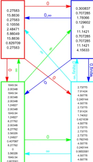
Figure 1 shows the resulting clusters obtained by applying our algorithm to the B&K fraternity data with n = 58 vertices. The data, collected by Bernard and Killworth, are behavioral frequency counts, based on communication frequencies between students of a college fraternity (see Bernard, H. R., Killworth, P. D. and Sayler, L., Social Science Research 11, 1982). When the data were collected, the 58 occupants had been living together for at least three months, but senior students had been living there for up to three years. Based spectral clustering considerations, we applied the algorithm withk= 4clusters. The four groups are likely to consist of persons living together for about the same time period.

While processing the iteration, occasionally we bumped into the situation when the degree sequence lied on the boundary of the convex polytopes defined in Sub- sections 2.1 and 2.2. Unfortunately, this can occur when our graph is large but not dense enough. In these situations the iteration did not converge for some co- ordinatesβiv (i∈Cu), but they seemed to tend to +∞or−∞. Equivalently, the correspondingbiv (i∈Cu)tended to+∞or 0, yielding the situation that member i∈Cu had+∞or 0 affinity towards members ofCv.

In Figure 1, we also enumerated the within-cluster parameter values for each cluster separately, and the parameters reflecting attitudes of students of one group towards the others were written in a concise form above the arrows, where 0,+∞, or finite parameter values can occur. The many 0 affinities show that some groups are quite separated, whereas some people in some groups show infinite affinity towards persons of some specific groups.

(8)

1

2 3 4

5 6 7

8 9

10

11 12

13 14

15 16 17 18

19

20 21

22

23 24

25

26 27

28

29

30 32 31

33 34

35

36 37

38

39

40 41 42

43

44

45 46

47

48 49

50

51

52

53 54

55 56

57 58

0.300837 0.707285 1.78066 0.129602 0 11.1421 0.707285 0.707285 11.1421 4.15633 0.27583

15.8836 0.27583 0.10556 2.48471 5.86049 15.8836 0.829709 0.27583

1049.54 2.00348 1049.54 2.00348 2.00348 1.24827 2.00348 1049.54 1.24827 8.27792 2.00348 8.27792 3.56026 1.24827 0.407567 8.27792 0 3.56026 1049.54 0.827001

2.73775 7.91424 4.50778 0.240144 4.50778 2.73775 7.91424 1.74052 0.421639 4.50778 2.73775 2.73775 2.73775 0.792745 4.50778 0.240144 0.0653581 4.50778 4.50778

0

0 0,∞

0,finite

0

∞

0

∞,finite,0

∞

Figure 1: The 4 clusters found by the algorithm and the within- and between-cluster affinities in the B&K fraternity data.

Acknowledgements. The authors thank Gábor Tusnády for fruitful discussions;

further, Róbert Pálovics and Despina Statsi for handing us real-world data to be processed.

References

[1] Chatterjee, S., Diaconis, P. and Sly, A., Random graphs with a given degree sequence,Ann. Stat., Vol. 21 (2010), 1400–1435.

[2] Csiszár, V., Hussami, P., Komlós, J., Móri, T. F., Rejtő, L. and Tusnády, G., When the degree sequence is a sufficient statistic, Acta Math. Hung., Vol. 134 (2011), 45–53.

[3] Csiszár, V., Hussami, P., Komlós, J., Móri, T. F., Rejtő, L. and Tusnády, G.,Testing goodness of fit of random graph models,Algorithms, Vol. 5 (2012), 629–

635.

[4] Dempster, A. P., Laird, N. M. and Rubin, D. B., Maximum likelihood from incomplete data via the EM algorithm,J. R. Statist. Soc. B, Vol. 39 (1977), 1–38.

[5] Rasch, G.,On general laws and the meaning of measurement in psychology. InProc.

of the Fourth Berkeley Symp. on Math. Statist. and Probab., University of California Press (1961), 321–333.

[6] Rinaldo, A., Petrovic, S. and Fienberg, S. E.,Maximum likelihood estimation in theβ-model,Ann. Statist., Vol. 41 (2013), 1085–1110.

[7] Ungar, L. H., Foster, D. P., A Formal Statistical Approach to Collaborative Filtering. InProc. Conference on Automatical Learning and Discovery (1998), 1–6.

Extending the Rash model to a multiclass parametric network model