submitted to the Doctoral Committee of the Hungarian Academy of Sciences

(1)

Numerical Investigations of Turbulent Structures in Fluids

Doctoral thesis

submitted to the Doctoral Committee of the Hungarian Academy of Sciences

G´abor Janiga, Ph.D.

2019

dc_1631_19

Powered by TCPDF (www.tcpdf.org)

(2)

dc_1631_19

(3)

Acknowledgements

I wish to record my sincere thanks to Professor Tibor Czibere for his creative influence on my professional activities and for his direct or indirect contribution to this work.

I acknowledge the support of Prof. Dominique Th´evenin which provided an environment in which all the ideas were developed.

I am also grateful to the numerous colleagues and coauthors in Miskolc and in Magdeburg over the years.

Special appreciation goes to my family, especially to my wife and my daugh- ter, for providing the necessary atmosphere of understanding and support during the untold amount of hours at home required for preparing this thesis.

iii

dc_1631_19

(4)

dc_1631_19

(5)

Acronyms

BPF Blade passage frequency

CFD Computational Fluid Dynamics CFL Courant-Friedrichs-Lewy (number)

DEISA Distributed European Infrastructure for Supercomputing Applications

DNS Direct Numerical Simulation

FDA Food and Drug Administration, USA HPC High Performance Computing

LDV Laser-Doppler Velocimetry LES Large Eddy Simulation MI Macro-instability

MRI Magnetic Resonance Imaging

NSCBC Navier-Stokes Characteristic Boundary Conditions NITA Non-Iterative Time Advancement

PC-MRI Phase-contrast Magnetic Resonance Imaging PIV Particle Image Velocimetry

POD Proper Orthogonal Decomposition PTV Particle Tracking Velocimetry RANS Reynolds-averaged Navier-Stokes SBES Stress-Blended Eddy Simulation

SPOD Snapshot Proper Orthogonal Decomposition SVD Singular Value Decomposition

URANS Unsteady Reynolds-averaged Navier-Stokes

v

dc_1631_19

(6)

dc_1631_19

(7)

Chapter 1 Introduction

Fluid flow problems play an important role in many practical applications, for example for energy generation, chemical engineering, biomedical flows or environmental problems. The fluid elements show a fluctuating and chaotic motion in the majority of these applications. The understanding and modeling of these so-called turbulent flows are much more challenging than laminar flows.

1.1 Introduction to Computational Fluid Dynamics

Fluid flow problems can be described by partial diﬀerential equations (see later in Chapter 2). Their analytical solution in a closed form exists only in special cases. These analytical solutions are particularly important to under- stand fluid flow phenomena, but they cannot be directly applied for solving real engineering problems.

Because of the enormous increase of computing capacity in the last decades the numerical solutions of partial diﬀerential equations are becoming more and more attractive. Parallel to the evolution of the computers, more and more advanced numerical methods have been developed. The immense progress in both computing hardware and numerical techniques led subsequently to the birth of the field which is today known as Computational Fluid Dynamics

1

dc_1631_19

(10)

2 1 Introduction

(or shortly CFD). In the frame of CFD the governing equations are solved numerically.

The numerical solution based on a discretization method translates the dif- ferential equations into a system of algebraic equation. This algebraic equation system can then be solved on computers. During the discretization the considered domain is divided into small parts, i.e., discrete points or discrete volumes.

The variables are calculated only at these discrete locations and are only defined on the numerical grid. It is the discrete representation of the considered continuous problem, obtained by dividing the computational domain into a finite number of small parts (control volumes or elements). If unsteady eﬀects are important, time is also considered as discrete time points. The accuracy of the obtained numerical solution is influenced by the characteristics of the applied discretization.

Three types of systematic errors can be distinguished, as described in [24]:

• Modeling errors: the diﬀerence between the actual flow and the exact solution of the mathematical model (wrong or incomplete physical models).

• Discretization errors: the diﬀerence between the exact solution of the conservation equations and the exact solution of the algebraic system of equations obtained by discretizing these equations.

• Iteration errors: the diﬀerence between the iterative and the exact solutions of the algebraic equation systems.

In addition, human errors should be mentioned, when applying inappropriate boundary conditions or wrong model settings.

The Navier-Stokes equations fully govern the flow of a viscous fluid. The same equation system can predict completely different flow configurations. Due to different boundary conditions, the same equation system dictates different solutions. Accurate and proper boundary conditions are especially important for CFD!

Three main solution approaches can be distinguished for solving numerical fluid flow problems. These are:

• finite diﬀerences [7, 63],

• finite volumes [24, 82],

• finite elements [56].

These techniques are partly similar, but also have their special features. All of these methods have advantages and disadvantages. Other dedicated techniques exist for special applications. In what follows, the finite volume method is applied in Chapter 3 and in Chapter 4. The finite diﬀerence method is con-

dc_1631_19

(11)

1.2 Modeling of Turbulent Flows 3

sidered in Chapter 5. These methods are not further discussed here. Excellent overviews are available in the already cited textbooks.

1.2 Modeling of Turbulent Flows

Depending on the value of a key non-dimensional number, the Reynolds number, every flow can be predicted to be laminar or turbulent. Turbulent flows can be found in most practical applications but are much more complex than laminar flows, because of their chaotic nature.

The increase in computing power and the development of numerical algorithms in recent decades has made CFD a widely used approach for complex engineering configurations. Nonetheless, progress in the modeling of the turbulent flows has not been that rapid.

In a high number of the engineering applications, the numerical solution still relies on the Reynolds-averaged Navier-Stokes (RANS) equations. In the RANS approach, each flow variable is decomposed into a deterministic time- average and a stochastic (turbulent) fluctuation. The purpose of RANS is the correct prediction of the time-averaged variables. Due to the averaging process underlying RANS, unknown correlation terms appear in the governing equations. These are the elements of the so-called Reynolds-stress tensor. The resulting number of unknowns is larger than the available number of equations, leading to the so-called closure problem [66]: in order to solve the system of equations a turbulence model is required. Widely used models are the k −ε and k −ω engineering turbulence models, as well as further variants derived from them [84]. These models still contain various model parameters, deduced from simple canonical flows.

These equations have been the subject of numerous studies over the last 50 years, but none of the RANS models have been determined to be superior for all types of flows without the use of some fine-tuning of the model parameters or constants (see, e.g., [78]). This could be due to the significant influence of the boundary conditions on the large energy-carrying turbulent eddies. Therefore, considering the dynamics of these eddies, the development of a universal RANS model might not be possible at all [59].

The direct numerical simulation (DNS) of the Navier-Stokes equations does not rely on any turbulence model. In this approach, the discretized governing equations are directly solved on a very fine computational grid with a large number of small time steps (see, e.g., [5]). All physically important scales are resolved – up to the so-called Kolmogorov scales – on the employed grid both

dc_1631_19

(12)

4 1 Introduction

in space and time. This very interesting method is still computationally pro- hibitive even for intermediate Reynolds numbers. In practice, this still remains challenging for everyday engineering problems, and will continue to be so even in the next decades despite of the rapidly increasing power of supercomputers.

The limitations of RANS and the unmanageable computational eﬀorts of DNS have led to the rapid development of large eddy simulations (LES), as a compromise between both [30, 71]. The LES approach spatially filters only the small-scale turbulent structures, which have less eﬀect on the overall energy budget. They can furthermore be considered as isotropic, and are therefore easier to model. At the same time, the large scale – anisotropic – structures are directly resolved on the employed grid, as in DNS. The spatial filtering again introduces unknown terms in the governing equations, the subgrid tensor. Since there are more unknown terms than the available number of equations, modeling is again required at the small scales, called the subgrid-scale (SGS) model.

Large eddy simulations can be considered as an intermediate approach between DNS and the solution of the RANS equations. In the past 15-20 years, LES has emerged and developed into a mature state in the study of turbulent flows including various mechanical, chemical and process engineering applications.

Generally speaking, LES simulations require a higher computational mesh resolution and shorter time steps than an unsteady RANS computation. Nev- ertheless, the computational eﬀorts are far lower than those required for DNS.

The continuous increase in computer resources makes LES more and more accessible for various engineering problems. When directly resolving at least 80% of the total amount of kinetic energy – a typical target for high-quality LES simulations [66] –, the obtained information concerning turbulent flows should be far more than that accessible by any RANS approach.

1.3 Outline

In this work, several turbulent flow problems are considered for various engineering applications involving CFD. All these problems result in a considerable computational eﬀort, therefore parallel computations are absolutely necessary.

This work is structured as follows. The governing equations are discussed in Chapter 2.

The flow prediction in a biomedical device is examined first in Chapter 3.

Although CFD is now extensively used for a broad range of industrial applica-

dc_1631_19

(13)

1.3 Outline 5

tions, but most medical scientists still do not consider CFD as a mature tool for biomedical flow simulations. In order to check this point, the FDA (Food and Drug Administration, USA) decided to propose several benchmark cases in order to study the validity and accuracy of CFD predictions for exemplary biomedical applications. A blood nozzle benchmark case is investigated in this work [79] considering Re = 6 500, since it is challenging from the point of view of the flow state. After the characterization of the diﬀerent flow regimes, the performance of a hybrid simulation is investigated in order to to reduce the computational costs.

In the second application example the time-dependent three-dimensional hydrodynamics in a stirred tank reactor is characterized by using numerical simulations (Chapter 4). The rotating propellers produce a complex, unsteady, three-dimensional turbulent flow field. This results in eﬃcient mixing and is therefore widely used in various process and chemical engineering applications.

The time-dependent turbulent single-phase flow is computed using large eddy simulation, relying on the sliding mesh approach. The dominant coherent flow structures are characterized in the entire three-dimensional computational domain by using the 3D proper orthogonal decomposition (POD) technique.

Furthermore, the macro-instability (MI) is examined by monitoring the fluid velocity in more than one million computational cells.

Applications involving turbulent flows with chemical reactions play an essential role in our daily life. All our transportation systems and the overwhelm- ing majority of our energy supply rely directly or indirectly on the combustion of fossil fuels. In order to improve the eﬃciency of such systems and to develop new approaches and configurations, numerical simulations play an increasing role in research and industry. They provide a cost-eﬃcient complement to experimental testing and prototypes. But, of course, they are only useful if they can accurately reproduce the real physical processes controlling practical configurations. Chapter 5 is devoted to the direct numerical simulation of turbulent premixed methane-air flames.

The new scientific results are summarized in Chapter 6.

dc_1631_19

(14)

dc_1631_19

(15)

Chapter 2 Governing Equations

2.1 Governing Equations of Reactive Flows

During the last decades, numerical combustion modeling has become a natu- ral complement to experiments, in particular to investigate in detail complex physical processes in realistic setups.

For a gas mixture the mass conservation and the Navier-Stokes equations can be written as:

∂ρ

∂t + ∂(ρuj)

∂x_j = 0 (2.1)

∂(ρu_i)

∂t + ∂(ρu_ju_i)

∂xj

=− ∂p

∂xi

+ ∂τ_ij

∂xj

, (2.2)

where ρ denotes mixture density, uj the components of the hydrodynamic velocity, p the pressure, and τij the stress tensor.

The additional balance equations expressing the conservation of chemical species and energy assuming ideal gas are given as:

∂(ρYk)

∂t + ∂(ρujYk)

∂x_j =−∂(ρYkVkj)

∂x_j + ˙ω_k; k = 1,2, ..., N_sp (2.3)

∂(ρe_t)

∂t + ∂[(ρe_t +p)u_j]

∂xj

=−∂q_j

∂xj

+ ∂(τ_iju_i)

∂xi

(2.4)

7

dc_1631_19

(16)

8 2 Governing Equations

p

ρ = R

WT , (2.5)

where N_sp the total number of chemical species, V_kj the component of the diﬀusion velocity of species k in the direction j, ˙ω_k the chemical production rate of species k and qj the j^th-component of the heat flux vector.

The stress tensor τ assuming a Newtonian-fluid:

τ_ij =µ

�∂ui

∂x_j + ∂uj

∂x_i

� +

�

−2 3µ

� ∂uk

∂x_kδ_ij (2.6)

with δ the Kronecker symbol (i.e., δ_ij = 1 if i =j and δ_ij = 0 otherwise) and µ the dynamic (or shear) viscosity.

2.2 Large Eddy Simulation of Non-reacting Flows

In the large eddy simulation (LES) approach the flow variables are decomposed using a filter to separate resolved scale – responsible for the large-scale inhomogeneous motions –, from subgrid scale – representing the small-scale, supposedly homogenous structures. The flow variables obtained in a large eddy simulation after the spatial filtering are denoted with the symbol ¯ . For an incompressible flow, as considered in Chapter 3 and Chapter 4, the filtered continuity equation reads:

∂u¯i

∂x_i = 0 (2.7)

and the filtered momentum equation for a Newtonian fluid can be written as:

∂

∂t (ρu¯i) + ∂

∂xj

(ρu¯iu¯j) = − ∂p¯

∂xi

+µ ∂

∂xj

�∂u¯_i

∂xj

+ ∂u¯_j

∂xi

�

− ∂τ_ij

∂xj

. (2.8) The fluid is considered here as isothermal, incompressible, and having New- tonian properties. The subgrid tensor τij is often expressed as the sum of the Leonard tensor, cross-stress tensor and Reynolds subgrid tensor [71]:

τ_ij =ρu_iu_j −ρu¯_iu¯_j =L_ij +C_ij +R_ij . (2.9) Most of the eddy viscosity models are given in the form:

τij − 1

3τkkδij =−2µtS¯ij , (2.10)

dc_1631_19

(17)

2.3 Reactive Flows 9

whereδ_ij is the Kronecker symbol (which is 1 if i= j, otherwise 0), µ_t is the – scalar – subgrid-scale turbulent viscosity, and the rate-of-strain tensor ¯S_ij for the resolved scale is given by:

S¯ij = 1 2

�∂u¯_i

∂xj

+ ∂u¯_j

∂xi

�

. (2.11)

CFD codes oﬀer various subgrid-scale models: the Smagorinsky [74] and the dynamic Smagorinsky-Lilly [54] models amongst others. The former is applied in the present work. The eddy viscosity in the Smagorinsky model is represented as:

µt =ρL²_s��S¯�� and ��S¯�� =

�

2 ¯SijS¯ij . (2.12) The original Smagorinsky model [74] does not consider zero eddy-viscosity for laminar shear flows. For wall-bounded flows, a damping factor depending on the wall-normal distance is applied in ANSYS Fluent. Hence, the mixing length L_s for subgrid scales in ANSYS Fluent is defined by [8]:

Ls = min�

κ d , CsV^1/3�

, (2.13)

whereκ is the von Kármán constant,d is the distance to the closest wall, V is the volume of the local grid element, and C_s is the non-dimensional coefficient called the Smagorinsky constant. The Smagorinsky constant Cs = 0.1 – the default value in ANSYS Fluent [8] – is retained for the presented cases in Chapter 3 and Chapter 4.

2.3 Reactive Flows

The basic notation commonly used in numerical combustion is introduced in this section considering a methane-air mixture.

The global reaction mechanism for a methane-air mixture is written as:

CH₄+ 2 (O₂ + 3.76 N₂)−→ CO₂ + 2 H₂O + 7.52 N₂ (2.14) The air is typically given as 1 mole of oxygen complemented by 3.76 moles of nitrogen. This single step reaction is composed of many elementary chemical reactions. The chemical mechanism of Smooke with 25 elementary reactions (Appendix A) is applied in Chapter 5 investigating methane-air flames.

dc_1631_19

(18)

In order to quantify the ratio of the fuel and the oxidizer in a methane-air mixture, the notation of mixing ratio α can be introduced. This mixing ratio is defined as the ratio of the mass flow rate of the fuel (methane) and the mass flow rate of oxidant (air):

α = m˙_CH₄

˙ mair

. (2.15)

The reaction is considered stoichiometric when the two flow rates are bal- anced, i.e., exactly the amount of oxidizer and fuel are used to completely burn.

The corresponding mixing ratio α_s – with the help of the molecular weights W – is:

αs = W_CH₄

2 (WO2 + 3.76WN2) . (2.16) The equivalence ratio φ of a methane-air mixture is defined as the ratio of mixing ratio α and α_s:

φ = α

α_s . (2.17)

A stoichiometric mixture has a value of φ= 1. A mixture containing an excess of methane is called rich flame (φ > 1), or it is lean if it contains an excess of air (φ < 1).

2.4 Description of the Gas Mixture

In the flame zone a large number of chemical species are involved in a complex process including many elementary reactions and possibly heat release. Some chemical species do not represent a large fraction of the whole mixture, but they may play an essential role in the reaction process as intermediate radicals [36].

The gas mixture is described using a predefined set of chemical species.

The complexity of this representation depends on the desired accuracy. The total number of chemical species taken into account in the reactive mixture is denoted Nsp.

The thermodynamic state of the gas mixture can be described by its composition, temperature and pressure. The composition of the mixture can be given by all the mass fractions of chemical species. Each species k is associated to its mass fraction Yk, which represents the mass of species k per unit mass of the mixture:

Y_k = ρ_k

ρ . (2.18)

dc_1631_19

(19)

2.4 Description of the Gas Mixture 11

The last species is supposed to be the dilutant (nitrogen in our applications) and its mass fraction can be deduced from the other mass fractions:

Nsp

�

k=1

Yk = 1 yields YN2 = 1−

Nsp−1

�

k=1

Yk . (2.19)

As a consequence, N_sp −1 transport equations must be solved to compute the composition of the reactive mixture. An additional equation will also be written for the energy balance. It is more usual to consider the specific enthalpy than the internal energy as the former is conserved through chemical processes at constant pressure and with adiabatic boundaries.

The mole fraction X_k of species k is defined by the ratio between the numbers of n_k moles of the given species k and the total number of moles n_t of the mixture:

Xk = n_k nt

. (2.20)

The average molar mass mixture of W is defined as follows:

W =

Nsp

�

k=1

XkWk , (2.21)

where W_k is the molar mass of species k.

The mass fractions and mole fractions are related by the following equality:

Y_k = W_k

W X_k . (2.22)

The average molecular weight of the mixture according mass fractions can also be expressed:

W =





Nsp

�

k=1

Y_k Wk





−1

. (2.23)

The enthalpy h of the mixture is given with the help of the species enthalpies, themselves being functions of temperature, specific heats at constant pressure cpk and of the standard formation enthalpies h⁰_k at standard temperature T0:

h=

Nsp

�

k=1

Ykhk (2.24)

dc_1631_19

(20)

and for each species:

h_k(T) = h⁰_k(T₀) +

� T

T0

c_pk(T^�) dT^� . (2.25) The enthalpy of mixture can also be written:

h=h⁰(T₀) +

� T

T0

c_p(T^�)dT^� , (2.26) where h⁰ is the enthalpy of mixture at the reference temperature:

h⁰(T₀) =

Nsp

�

k=1

Y_kh⁰_k(T₀) (2.27)

and cp is the average specific heat of the mixture given by:

cp =

Nsp

�

k=1

Ykcpk . (2.28)

2.5 Chemical Reactions

The detailed chemistry method is applied to describe the reaction processes in Chapter 5, therefore, it is discussed next.

The overall chemical mechanism is modeled by I elementary reactions involving maximum 3 reactants and 3 products. Each elementary reaction (using index i) can be written as:

Nsp

�

k=1

ν_ki^� X^k �

Nsp

�

k=1

ν_ki^��X^k (2.29)

with ν_ki^� and ν_ki^�� as stoichiometric coeﬃcients (0 for most species or 1, maximum 2) The molar production rate of one species k per unit volume is given as:

˙ ωk =

�I i=1

(ν_ki^�� −ν_ki^� )



kfi

N�sp

k=1

[X^k]^ν^ki^� −kri

N�sp

k=1

[X^k]^ν^ki^��



 , (2.30)

dc_1631_19

(21)

2.6 Proper Orthogonal Decomposition (POD) 13

where [X^k] is the concentration of species k and the forward and backward rates of progress of each reaction (k_f_i and k_r_i) are related to each other via the reaction equilibrium constant. These rates are modeled by the Arrhenius law:

k_f_i =A_iT^βⁱ exp

�−E_i R T

�

(2.31) and

kr_i = k_f_i Kei

. (2.32)

The equilibrium constant Kei can be determined from the standard enthalpy and entropy as a function of temperature.

For all reactive flow computations presented in Chapter 5, the complete set of chemical species and elementary reactions, with their Arrhenius coeﬃcients Ai, βi and Ei, is taken from [12, 75] (Appendix A).

2.6 Proper Orthogonal Decomposition (POD)

Proper orthogonal decomposition (POD) is a promising method for the analysis and synthesis of experimental or computational data. It serves also a basis for the determination of low-dimensional dynamic models of complex systems, see, e.g., [39]. Considering only a few modes, a large amount of kinetic energy can be captured. It allows for reduced order models of a complex spatial-temporal system to be built. Conveniently, POD analysis is a linear procedure, nonetheless, it can be applied for non-linear systems without assuming linearity.

The classical proper orthogonal decomposition introduced by Lumley [58]

considers the spatial correlation of the flow field realization. The solution of the system involves a singular value decomposition (SVD), therefore, this method is also referred as the SVD method. In practice, this method is limited to moderate spatial resolution – especially for two-dimensional experimental data – because of the computational expenses.

The alternative POD realization, introduced by Sirovich [73], takes the temporal correlation into consideration. This approach is often referred to as snapshot POD or briefly SPOD. The SPOD method is computationally more beneficial for a larger spatial resolution.

Both of these methods have been extensively analyzed and compared for complex flows in two-dimensional planes – involving both two and three ve-

dc_1631_19

(22)

locity components – in [9]. The purpose of the current work is to investigate complex three-dimensional flows, therefore, the two-dimensional SPOD imple- mentation applied in [9] is extended for three-dimensional domains.

The POD technique oﬀers a broad range of applications in fluid dynamics.

It can be used to compare diﬀerent time-varying three-dimensional flow data [45]. The POD analysis supports the feature-based visualization, where the most energetic flow features can be extracted [44]. According to Lumley [58]

the flow representation having a largest projection onto the flow defines the coherent flow structures. A given coherent structure is an eigenmode of the two-point correlation matrix of the snapshot database.

The computational details of both the SVD and the SPOD methods are detailed in [9]. Here, only a the SPOD method is briefly summarized.

2.6.1 Snapshot POD Method

The developed method was inspired by Snapshot Proper Orthogonal Decom- position (SPOD, see [73]), but for a completely different objective. The funda- mental idea behind POD is to decompose each signal u(x, t_k) into orthogonal deterministic functionsφ(POD spatial modes) and time-dependent coefficients a_k (POD temporal coefficients):

u(x, t_k) =

�∞ l=1

a^l_kφ^l(x) . (2.33)

Here, superscript l and subscript k refer to the mode number and index of corresponding snapshot (or time step), respectively. The function φ denotes the eigenfunction of the Fredholm integral equation

�

X

R(x,x^�)·φ(x^�) dx^� =λφ(x) . (2.34) The kernel of this eigenvalue problem is the two-point spatial correlation function

R(x,x^�) = �u(x, tk)⊗u(x^�, tk)�t , (2.35) where t_k and x are snapshot time and position vector, respectively. In POD, φ is chosen to maximize the value of �

|(u, φ)|²�

/� φ�², where �·�t, �·�, (·,·) and � · � are time average, spatial average, inner product and norm, respec-

dc_1631_19

(23)

2.6 Proper Orthogonal Decomposition (POD) 15

tively. Since the spatial modes φ^l are orthonormal to each other, the following equation can be used

φ^l(x) =

Ns

�

k=1

a^l_k u(x, tk) . (2.36) In order to determine the coeﬃcients a_k, Eq. (2.36) is substituted into Eq. (2.34), resulting in

� 1 Ns

Ns

�

i=1

u(x, ti)⊗u(x, ti),

Ns

�

k=1

aku(x, tk)

�

=λ

Ns

�

k=1

aku(x, tk) ,

whereN_sis the total number of snapshots. Sirovich [73] simplified this equation into

Ns

�

k=1

1 Ns

(u(x, ti),u(x, tk))ak = λai ; i = 1, ..., Ns . (2.37) Equation (2.37) can be rewritten in symbolic form as:

CA =λA, (2.38)

A = (a₁, a₂, ..., a_N_s)^T , (2.39) Cij = (u(x, ti),u(x, tj))

N_s . (2.40)

Solving this eigenvalue problem, Eq. (2.38), leads to a total of Ns eigenvalues, written λ^l, and eigenvectors, denoted A^l (l ∈ 1,2,3, ..., Ns). When using SPOD for data analysis or data compression, it is not always necessary to keep all N_s modes. Then, M represents the number of modes retained in the analysis whileNs still represents the total number of snapshots, i.e., the whole data-set available for the analysis, obviously with M ≤Ns.

2.6.2 Spectral Entropy

Equation (2.37) describes in general the eigenvalue problem based on the temporal autocorrelation function as kernel. The obtained eigenvalues represent the spectrum of the autocorrelation matrix (C in Eq. (2.38)). In order to

dc_1631_19

(24)

characterize the intensity of the turbulence contained in the analyzed velocity field u, the spectral entropy S_d can be introduced. This quantity allows one to distinguish between diﬀerent flow regimes, from “highly disordered” (here, meaning turbulence), to “partially ordered” (here, for transition), or “well ordered” (here, for laminar flow). For the computation of the spectral entropy, the relative energy P^l of mode l is first computed based on the corresponding eigenvalue, after ordering them in decreasing order based on λ^l, as:

P^l = λ^l

�M j=1

λ^j

, (2.41)

where M ≤ Ns is the number of modes retained in the analysis. Then, the spectral entropy can be determined as:

Sd =−

�M

l=1

P^l lnP^l . (2.42)

According to Eq. (2.42), the maximum possible value of S_d is reached when all eigenvalues are equal to each other, i.e., P^l = 1/M, and consequently Sd = ln(M). Physically, this means that the energy is equally distributed over all the M modes. The minimum value of S_d corresponds to the case where the original signal contains only a single mode, the first one, meaning that the flow field is steady. Then, S_d = 0.

dc_1631_19

(25)

Chapter 3 Large eddy simulation of the FDA benchmark nozzle

This chapter investigates the flow in a benchmark nozzle model of an idealized medical device using computational fluid dynamics (CFD). It was proposed by the Food and Drug Administration (FDA) [31]. It will be shown that a proper modeling of the transitional flow features is particularly challenging, leading to large discrepancies and inaccurate predictions from the diﬀerent research groups using Reynolds-averaged Navier-Stokes (RANS) modeling [79].

In spite of the relatively simple, axisymmetric computational geometry, the resulting turbulent flow is fairly complex and non-axisymmetric, in particular due to the sudden expansion. The resulting flow cannot be well predicted with simple modeling approaches. Due to the varying diameters and flow velocities encountered in the nozzle, diﬀerent typical flow regions and regimes can be distinguished, from laminar to transitional and to weakly turbulent. The purpose of the present chapter is to re-examine the FDA-CFD benchmark nozzle model at a Reynolds number of 6 500 using large eddy simulation (LES) [42].

The LES results are compared with published experimental data obtained by Particle Image Velocimetry (PIV) and an excellent agreement can be observed considering the temporally-averaged flow velocities. Diﬀerent flow regimes are characterized by computing the temporal energy spectra at diﬀerent locations along the main axis [17]. In order to reduce the computational costs, the performance of a hybrid simulation is investigated [17].

17

dc_1631_19

(26)

18 3 Large eddy simulation of the FDA benchmark nozzle

3.1 Introduction

The Food and Drug Administration (FDA) is responsible in the USA for the authorization and control of new medical devices. Their mission is to protect

“the public health by assuring the safety, eﬃcacy and security of human and veterinary drugs, biological products, medical devices” ¹. In this process results based on computational fluid dynamics (CFD) are becoming more and more important to demonstrate the eﬃcacy and safety of new technologies and products. Though CFD is widely used and accepted in various engineering fields, the relevance and accuracy of CFD is still questioned in part of the biomedical community [50, 77]. This is one reason why FDA decided to propose a benchmark case to check the validity and accuracy of CFD predictions for a typical biomedical application (Fig. 3.1). A total of 28 CFD groups from all around the world have participated to this benchmark, performed the required computational steps and delivered the results for a later analysis [79]. Comple- mentary experimental investigations [31] – using blood-analog fluids to match the refractive index of the acrylic geometry – were also performed using Parti- cle Image Velocimetry (PIV) in order to generate a reference database for the CFD validation. However, the experimental results were not known prior to the simulations (blind predictive test). The aim of the FDA-study was to evaluate the current state of the art in CFD modeling in an idealized medical device model, specifically: “(1) develop a suitable benchmark model for the interlaboratory study (as well as for future research and standards development); (2) evaluate and compare each participants CFD simulations against quantitative flow visualization experiments carried out in three independent laboratories;

and (3) extract needed input for the development of standards and guidelines for industry and FDA reviewers who employ or consider CFD in premarket device applications and postmarket investigations of device problems” [79].

Comparing the CFD results with the experimental data, large discrepancies were observed among the numerical predictions [79]. The discussed results involved both laminar as well as turbulent simulations for five diﬀerent Reynolds numbers ranging from Re = 500 to Re = 6 500, using as typical length-scale the throat diameter. The computational geometry is otherwise identical for all cases (Fig. 3.1).

The investigated configuration is axisymmetric and can in principle be computed as an axisymmetric domain without swirl (2D), greatly reducing the computational eﬀorts. None of the contributed CFD results relied on large eddy simulation, probably due to the much higher computational eﬀort. In-

1 http://www.fda.gov/AboutFDA/WhatWeDo/

dc_1631_19

(27)

3.1 Introduction 19

damage and thrombus formation! based on the purely physical results "e.g., pressures, velocities, and shear stresses! of the simulations. We initiated a collaborative project to determine the current state and limitations of CFD modeling and the blood damage estimations, as applied to medical devices. The project is part of the FDA’s “Critical Path Initiative” program, which is a “national strategy for driving innovation to modernize the sciences through which FDA-regulated products are developed, evaluated, manu- factured, and used” #18$. In essence, the goal of our project is to work with the medical device community to improve the use and validation of CFD techniques in medical device evaluation to fos- ter the development of better and safer products and technologies.

In collaboration with researchers experienced in both CFD and particle image velocimetry "PIV! as applied to medical devices, a benchmark nozzle model was developed, which contained features commonly encountered in medical devices "including regions of flow contraction and expansion, local high shear stresses, flow recirculation, and flow regimes that ranged from laminar to turbulent!, yet was simple enough that CFD analyses could be readily performed and meaningful comparisons made. By partner- ing with multiple technical societies, the international CFD community was invited to perform independent simulations of the nozzle model. In response, participants from 28 different groups submitted CFD results #19$. To validate the computational flow simulations, interlaboratory flow visualization experiments at three different laboratories were performed on fabricated physical models. Comparisons of the interlaboratory PIV data allowed us to perform an error analysis, which is a critical component of CFD validation. In addition, to validate the blood damage predictions from the CFD simulations, interlaboratory blood damage experiments were performed at three independent facilities, results of which will be presented in a future report.

This paper addresses three important goals of the FDA CFD blood damage project. The first is to present a benchmark device and an experimental protocol for performing PIV measurements that can be used to validate CFD simulations. The second is to present some noteworthy aspects of the measured data, including some that are particularly subtle and hence deserving of extra attention in CFD validations or further PIV experiments to con- firm the results. The third goal is to make these benchmark data available to the scientific community through an online repository for use in future CFD validation studies. The CFD round-robin results as well as the PIV validation of the CFD results will be presented in later publications.

PIV has been widely used in evaluating the performance of medical devices such as artificial heart valves #20–26$, blood pumps #27–34$, and stents#35,36$. Viscous and Reynolds stresses estimated from PIV have been used to predict the blood damage potential of various medical devices #20,23,25,28,30$. PIV uses an array of computational tools "e.g., cross-correlation algorithms, image processing, and statistics! to estimate the velocity at multiple locations in a flow field. Consequently, the accuracy of the PIV technique depends on the quality of the images, the spatial and temporal image resolutions, and the number of images used, as well as the particle size, particle seeding density, particle dis- placement, and the ability of the particles to follow the flow. Dif- ferences in the PIV algorithms can also significantly influence the accuracy of the predicted flow quantities. An international PIV challenge with more than 23 participating groups² investigated the accuracy of different commercial and open-source PIV algorithms by conducting three different round-robin studies with common image sets #37$. A majority of the participants demonstrated the capability of PIV to accurately measure mean "time-averaged! velocities. However, they also acknowledged the limitations of some of the PIV algorithms in measuring turbulent characteristics, as well as velocities and shear stresses for flows near walls #37$.

Furthermore, the accuracy and reproducibility of PIV experiments

are affected not only by the algorithms used, but also by experimental factors such as fluctuations in the flow conditions and fluid properties, as well as uncertainties associated with measurements of fluid properties, all of which can vary from one laboratory to another. Controlling these variables to accurately generate the desired flow field is absolutely critical to obtaining accurate esti- mates of the velocity and stress fields.

To minimize the user error and laboratory bias due to these issues, a standard operating procedure "SOP! for performing the PIV measurements was collaboratively developed in this study.

Following the SOP, velocity, pressure, viscous shear stress, and turbulent Reynolds stress data were obtained by the participating laboratories at select cross-sectional locations in the nozzle model.

The cross-sections were chosen to appropriately capture the different flow phenomena occurring in the nozzle. Subsequently, an error analysis for the interlaboratory PIV measurements was performed. The error analysis included estimating the uncertainty in the measurements among the laboratories due to differences in PIV algorithms, inlet flow conditions, and fluid property measurements. The combined results from the PIV experiments will be used to evaluate the capability of the CFD simulations to numerically predict the flow fields.

Section 2 describes the benchmark nozzle model and the experimental protocol for the PIV experiments. Uncertainties in the PIV measurements are quantified in Sec. 3.1. Select velocity measurements from all three laboratories are presented in Sec. 3.2.

Finally, the applicability of the interlaboratory PIV results for validating the round-robin CFD data is assessed in Sec. 4.

2 Materials and Methods

2.1 Nozzle Model. The benchmark nozzle model is similar to previously reported designs used to compare blood damage computations to experimental data #8,12,38–42$. The model has characteristics of medical devices that have blood flowing through them, including hemodialysis tubing sets, catheters, cannulae, sy- ringes, and hypodermic needles. The nozzle incorporates on one end a 20 deg conical section that gradually reduces the inlet diameter from 12 mm to 4 mm in the nozzle throat; the opposite end is characterized by a sudden increase in diameter "Fig. 1!. With flow in one direction, the device resembles a conical concentrator and a sudden expansion "referred to as the “sudden expansion model”!. With flow in the opposite direction, the nozzle models a sudden contraction and a conical diffuser "referred to as the “conical diffuser model”!. This paper will concentrate on flow through the sudden expansion model, although the experimental results for the conical diffuser model are also available elsewhere.³

For performing PIV experiments, three identical nozzle models

"one for each of the three laboratories! were fabricated from cast

acrylic using an MB-46VAE three-axis computer numerical con- trolled "CNC! milling machine "Okuma Ace Center, Charlotte, NC!. After internal machining and annealing to relieve residual material stresses, the planar external surfaces of the models were

2http://www.pivchallenge.org/ ³http://fdacfd.nci.nih.gov

Fig. 1 Benchmark nozzle model: schematic of the test section with dimensions

041002-2 / Vol. 133, APRIL 2011 Transactions of the ASME

Downloaded 17 Feb 2011 to 150.148.0.65. Redistribution subject to ASME license or copyright; see http://www.asme.org/terms/Terms_Use.cfm

Flow direction

z

z = 0 cm

1.2 cm d = 0.4 cm

Throat

1.2 cm 2.2685 cm

4 cm

Fig. 3.1: Schematic representation of the computational domain for the FDA- benchmark nozzle model. [17] [31] [42]

stead, the CFD simulations discussed in [79] rely on laminar and Reynolds- averaged Navier-Stokes (RANS) models involving both steady and transient as well as two- and three-dimensional computations.

In their conclusion, the FDA-experts “do not endorse or recommend the use of any particular turbulence model over any other”, raising in particular the question: could large eddy simulation outperform the presented laminar and RANS computations? In what follows only the highest Reynolds number considered in the FDA study (Re = 6 500) based on throat diameter is investigated using large eddy simulation [42]. This case is challenging since it clearly involves transition and noticing that “minor flow rate variations can have a substantial eﬀect on the nature of the flow” [79]. This particular Reynolds number in the original study has been investigated by several groups, two of them assuming a laminar flow, the remaining ones using three diﬀerent turbulence models, namely: Spalart-Allmaras in one case, k −ω in three studies, k−ω SST in 12 studies and k −� in 10 computations.

For engineering applications at very high Reynolds numbers, it is very challenging to obtain the needed resolution in space and time. In the present case, the Reynolds number Re = 6 500 based on throat diameter is still moderate, so that a proper resolution can be obtained. The aim of the present chapter is thus to re-investigate the FDA benchmark nozzle using LES and check the accuracy of the obtained results [42].

dc_1631_19

(28)

3.2 Methods

3.2.1 Computational Mesh

In order to eliminate any spurious influence of the inlet and outlet boundary conditions, the considered geometry (Fig. 3.1) has been extruded at both ends of the considered domain, especially at the outlet. A previous test with a shorter domain has shown a recirculation at the outlet for the investigated Reynolds number. Therefore, the final computational domain is selected to be 9 cm long between the sudden expansion and the outlet, while the complete computational domain is almost 20 cm long.

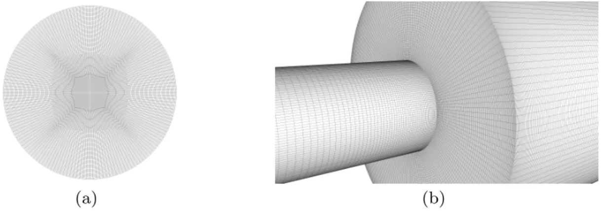
The applied computational mesh needed for the finite-volume simulation has been generated using the commercial tool ICEM-CFD (Ansys Inc., Canons- burg, PA, USA). The block-structured mesh involves 9 129 600 finite-volume cells composed of hexahedral elements using two combined O-grid topologies [42]. An example of the computational mesh used for the present case is shown in Fig. 3.2. For all the mesh elements the orthogonal quality is better than 0.7 (1 being the highest) and the equi-angle skewness is better than 0.5 (1 being the worst and 0 the optimum), leading to an excellent overall mesh quality.

The volume of the smallest grid volume elements, which are found in the region near the expansion, is 1.5×10⁻⁵ mm³, corresponding to a cell size of 24×24×25 µm. An extremely fine resolution has been implemented in the vicinity of the walls. The wall normal grid distance is between 7.5 and 27.5 µm providing a near-wall resolution less than one in wall units [42].

The largest computational cells are located near the inlet and outlet. The resolution is gradually refined approaching the two ends of the throat section.

An extremely fine resolution is provided at the level of the sudden expansion, which has been found to be very important in order to resolve correctly the flow separation [42]. The boundary layer is fully resolved in the present work and is thus not modeled as common in a RANS approach. This direct resolution is hardly possible for high Reynolds numbers, but is feasible for a moderate Reynolds number as in the present case. The final mesh resolution is mainly guided by the wall resolution and having almost homogeneous cells in the core of the domain.

dc_1631_19

(29)

3.2 Methods 21

(a) (b)

Fig. 3.2: Block-structured computational mesh for the FDA benchmark nozzle (a) two combined O-grid topologies at the outlet of the domain (b) refined mesh near the sudden expansion. [42]

3.2.2 Computational Details

The fluid flow simulations have been performed using the commercial finite- volume solver ANSYS Fluent 14 (Ansys Inc., Canonsburg, PA, USA) applying the double-precision pressure-based solver [42].

The inlet boundary condition for the velocity is prescribed in the form of a steady laminar parabolic profile. Note that the Reynolds number computed from the entry diameter is only Re = 2 167, denoting laminar conditions and therefore justifying this assumption. As a consequence, the observed complex unsteady flow downstream the sudden expansion is directly a result of the local flow instability associated to transition (Re = 6 500 when computed with the throat diameter).

Traction-free conditions are implemented at the outlet, assuming an identical uniform relative pressure. A standard, no-slip boundary condition is employed along the walls. [42]

The fluid is represented using isothermal and incompressible Newtonian blood properties. The constant density and the dynamic viscosity are chosen as 1056 kg/m³ and as 3.5 mPa·s, respectively [79].

Computations are carried out in parallel using 32 Linux computing cores on eight quad-core computing nodes equipped with AMD Opteron 64-bit Pro- cessor 2352 having 2.1 GHz clock rate. Each node has 32 GB memory and the internode communication is realized with a high-speed InfiniBand connection.

For the mesh considered in this study, over 20 GB of computer memory are needed for the simulation. The complete numerical simulations are finished

dc_1631_19

(30)

in around 470 hours wall-clock-time, corresponding to almost 20 days on 32 computing cores in parallel. [42]

The time advancement is realized using the Non-Iterative Time Advance- ment (NITA) based on the Fractional Time Step method with an implicit second-order scheme.

The convective terms in the momentum equations are discretized with a second-order central diﬀerencing scheme and the Least Squares cell-based approach is employed for the interpolation of variables on cell faces.

A constant time step of 10⁻⁵ s ensures that the Courant-Friedrichs-Lewy (CFL) number is less than unity everywhere. Before starting the averaging procedure in time, the simulation was continued for more than 50 000 time steps, corresponding to three through-flow times from inflow to outflow of the computational domain. All the presented profiles are the results of time- averaging performed during 100 000 time steps (almost 7 through-flow times), ensuring converged statistics. [42]

3.3 Results

Exemplary instantaneous velocity magnitudes are shown in Fig. 3.3(a). A computed iso-surface of the Q-criterion for Q= 2×10⁶ 1/s colored with the same axial velocity is shown in Fig. 3.3(b). The topology of this quantity reveals the existence of strong coherent structures in the considered flow showing a periodic street of vortex rings downstream the nozzle. Fig. 3.4(a) shows the instantaneous velocity magnitudes in a two-dimensional cut in the middle of the geometry. The high velocity regions shown in red color downstream the sudden expansion reveal the coherent ring-shaped structures produced peri- odically. Fig. 3.4(b) presents the computed vorticity magnitude in the same cut plane and at the same time step, showing the jet flow and highlighting the strong interaction between the near-axis high-speed jet and the stagnating flow in the recirculation.

These figures illustrate the complexity of the turbulent structures induced by the sudden expansion in this rather simple geometry. The resulting, highly unsteady flow cannot be directly compared with transient experimental results, because of the stochastic nature of turbulence. Nevertheless, all the re- alizations should give the same results in a statistical sense. Therefore, the temporally-averaged computational results are compared next with the averaged experimental results.

dc_1631_19

(31)

3.3 Results 23

(a) (b)

Fig. 3.3: Various representation of the instantaneous turbulent flow at Re = 6 500 in the nozzle. (a) Volume rendering of instantaneous velocity magnitude and (b) corresponding iso-surface of the Q-criterion colored by the axial velocity. [42]

Experimental data have been obtained by independent PIV measurements in three different laboratories [31]. As discussed in [31], the different groups observed either laminar or transitional flows even before reaching the throat for the considered Reynolds number. These different observations for the same configuration point out to one of the main difficulties of the present case.

While Re = 6 500 corresponds clearly to turbulent conditions in the throat section, the corresponding Reynolds number computed with the diameter of the baseline pipe is Re = 2 167, very close to the value associated to transition (Rec ≈ 2 300), so that laminar or transient conditions might be found due to spurious eﬀects, like slight vibrations in the surroundings. Even very small dis- turbances might be amplified and lead to diﬀerent experimental observations.

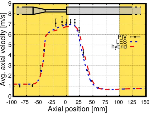
All experimental results shown in what follows, for instance in Fig. 3.5, are the averaged values obtained by the three laboratories reported in [31]. The error bars represent the deviation between the diﬀerent measurements (min- max range). Fig. 3.6 depicts the computed time-averaged axial velocity along the centerline [42]. The symbols illustrate the average of all PIV experiments.

The deviation is again shown by error bars.

dc_1631_19

(32)

(a)

(b)

Fig. 3.4: Instantaneous turbulent flow at Re = 6 500 in the middle plane of the nozzle. (a) instantaneous velocity magnitude in a two-dimensional cut-plane and (b) corresponding values of vorticity magnitude. [42]

In the present computations a steady laminar inflow (parabolic) profile is prescribed at the inlet of the domain. No artificial turbulence fluctuations are superimposed at the inlet, as it is often required for LES computations at high Reynolds numbers. Hence, all the unsteady flow features observed downstream are solely a result of transition within the considered geometry. [42]

Most of the temporally-averaged axial velocity profiles show fully symmetric curves (Fig. 3.5). For the last two measured sections (z = 0.060 and z = 0.080 m in Fig. 3.5) velocities are not yet fully symmetric, despite of the long averaging time [42]. Indeed, these profiles are located in the relaminarization region. Because the Reynolds number there is very close to the critical Reynolds number, the full relaminarization of the flow takes a considerable time and could only be observed further downstream, leading to exceedingly high computational costs.

3.3.1 Turbulent Velocity Spectra

In order to characterize the diﬀerent flow regimes, turbulent spectra are now investigated. Various probe locations along the centerline of the geometry have

dc_1631_19

(33)

3.3 Results 25

Axial direction, z/D [-]

0 2 4 6 8 15 20

D

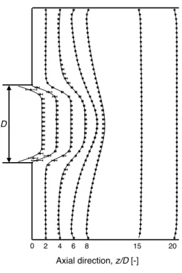
Fig. 3.5: Time-averaged axial velocity compared with PIV measurements along various cuts near the sudden expansion. Experimental values are plotted with symbols, solid lines represent the averaged, resolved axial velocities obtained by LES. For a better visibility, only a part of the computational domain is considered. [42]

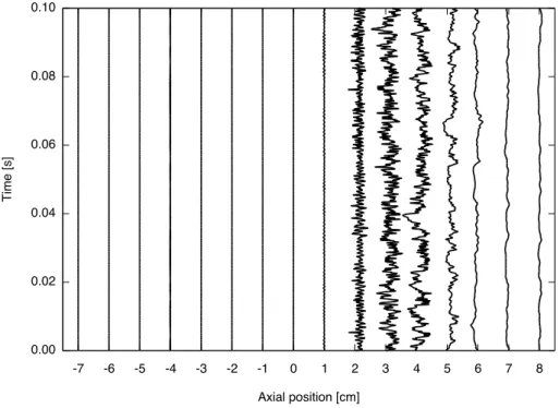
been defined. At these points the instantaneous axial velocity components are stored during the last 10 000 computational time steps. The first probes (left part of Fig. 3.7) are placed before the convergent nozzle, and no oscillations are visible. The next probes, located within the convergent nozzle, show a slight periodic oscillation with amplitude modulation. Then, the probes located downstream the sudden expansion (at z = 0) show clearly unsteady transitional behavior, before relaminarization occurs (right part of Fig. 3.7). [42]

The corresponding spectra of turbulent kinetic energy have been computed at these same locations and are shown in Fig. 3.7. These logarithmic plots illustrate the turbulent kinetic energy as a function of the Strouhal number St.

Spatial correlations are usually presented as a function of the wave number, while the temporal correlations are plotted against the frequency or Strouhal number. According to Kolmogorov [51] the energy spectra can be well ap-

dc_1631_19

(34)

0 1 2 3 4 5 6 7 8

-25 -20 -15 -10 -5 0 5 10 15 20

Axial velocity [m/s]

Axial direction, z/D [-]

PIV LES

Fig. 3.6: Time-averaged axial velocity compared with PIV measurements along the centerline. Experimental values are plotted with symbols, the solid line represents the averaged, resolved axial velocity obtained by LES. [42]

proximated with a −5/3 slope [38] in the so-called inertial subrange for high Reynolds numbers. [42]

The constant laminar values at the first probes do not lead to any noticeable turbulent kinetic energy content, as expected. Within the throat, the induced slight oscillations are associated with a limited amount of kinetic energy in Fig. 3.7, indicating the onset of the transitional stage of the flow. Downstream of the sudden expansion, the flow is clearly turbulent, and part of the spectra can be very well approximated with a slope of −5/3, even if a large part of it can be still better described by a slope of −10/3. Far from the sudden expansion the kinetic energy decays and the obtained spectra show a decreasing amount of energy. The−10/3 slope becomes more and more important in these region, representing the viscous dissipation subrange indicating high-frequency turbulent motions. [42]

dc_1631_19

(35)

3.4 Discussion 27

Fig. 3.7: Instantaneous axial velocity values at various locations along the centerline. [42]

3.4 Discussion

The presented results are not obtained from a blind test as those discussed in [79]. The measurement results were available before starting the LES computations. However, no modification of the models was needed to improve the comparisons. The results are obtained using a high-quality, well-resolved mesh with appropriate time steps, and this was found to be suﬃcient. No further parameters – e.g., the Smagorinsky constant – had to be adapted in order to improve the results.

The temporally averaged axial velocity profiles have been obtained experimentally by PIV [31]. These results could not be well reproduced by any of the RANS simulations discussed in [79]. Here, as observed when looking back at Fig. 3.5, a truly excellent agreement can be observed in all regions of the geometry, before, within and after the throat. In particular, the obtained LES results predict well the velocity profiles after the sudden expansion, in spite of the complex turbulent nature of the fluid flow illustrated for instance in Fig. 3.3.

dc_1631_19

(36)

It is known that symmetric diﬀusers may lead to separation on one side and attachment on the other side. Therefore, a non-symmetric flow can develop within a truly axisymmetric configuration. This might be a problem for the considered benchmark nozzle and explain why the transient and turbulent flows are not always axisymmetric, as shown exemplary in Fig. 3.3. This might also be one reason for the poor agreement with experimental data documented in [79], since this behavior obviously cannot be predicted by two-dimensional axisymmetric computations.

Another reason for the discrepancies discussed in [79] is that unsteady RANS simulations cannot really predict all the diﬀerent flow regimes encountered in the considered application, from laminar to turbulent through transition. A wall-resolved LES based on the standard Smagorinsky model [74]

model with wall damping delivers an excellent agreement compared with experiments in the present study.

The velocity spectra obtained in the current simulation have been presented in Fig. 3.7. The observation are consistent with the −5/3 power law representing the inertial range in the theory of Kolmogorov, even if this applies only to a small region. The largest part of the spectra beyond the sudden expansion can be well represented with a slope around −3 or −10/3 [42]. A slope of

−10/3 has been observed experimentally for stenotic conditions at relatively low Reynolds numbers [57]. Molla et al. [60] reported a combination of slopes

−5/3 and −10/3 in a modeled stenosis using LES computations. They observed that the slope of −10/3 was more pronounced in the relaminarization regime. In the current work the kinetic energy spectra are mostly characterized with the slopes of −5/3 and −10/3, showing that even small-scale vortical structures appear to be well resolved.

These observations demonstrate that the resolution of the employed LES computations is suﬃcient.

3.5 Hybrid Simulations

Hybrid simulations might be very interesting to save computational resources for a variety of applications involving diﬀerent flow regimes. Combining proper models for laminar, transitional, or turbulent flows, described either by steady RANS, unsteady RANS (URANS), LES or DNS depending on the needs, an accurate solution could then be obtained for complex configurations on existing computers. To do so, it is necessary to decide which kind of model should be used in which part of the numerical domain in space and time. As shown

dc_1631_19