Hybrid Feedback Linearization Slip Control for Anti-lock Braking System
Samuel John
1, Jimoh O. Pedro
21 Department of Mechanical Engineering The Polytechnic of Namibia
P. Bag 13388, Windhoek Namibia Email: sjohn@polytechnic.edu.na
2 School of Mechanical, Industrial and Aeronautical Engineering The University of the Witwatersrand
P. Bag 3, Johannesburg, South Africa Email: jimoh.pedro@wits.ac.za
Abstract: The Anti-lock braking system (ABS) is an active safety device in road vehicles, which during hard braking maximizes the braking force between the tyre and the road irrespective of the road conditions. This is accomplished by regulating the wheel slip around its optimum value. Due to the high non-linearity of the tyre and road interaction, and uncertainties from vehicle dynamics, a standard PID controller will not suffice. This paper therefore proposes a non-linear control design using input-output feedback linearization approach. To enhance the robustness of the non-linear controller, an integral feedback method was employed. The stability of the controller is analysed in the Lyapunov sense. To demonstrate the robustness of the proposed controller, simulations were conducted on two different road conditions. The results from the proposed method exhibited a more superior performance and reduced the chattering effect on the braking torque compared to the performance of the standard feedback linearization method.
Keywords: anti-lock braking system; wheel slip; friction model; hybrid systems; feedback linearization; PID
1 Introduction
The anti-lock braking system is a device that senses when the wheels of a vehicle are about to lock during hard-braking and it releases the brakes, so that locking of wheels does not occur. This operation results in the improvement of the longitudinal stability and hence the driver's steering control, thereby improving the driver's ability to avoid obstacles. In addition, the action of the ABS results in maximizing the frictional forces between the tyres and the road, consequently
minimizing the braking distance. Most commercial ABSs have a design objective of maximising the friction force between the tyres and the road surface to achieve shorter braking distance and better steering control [1, 2]. They are implemented using an algorithm that is based on complicated logic rules (table rules) that attempt to capture all possible operating scenarios. These rules are executed by a control computer that switches on and off solenoid valves to ensure the right pressures are delivered to the wheels while avoiding slippage [3]. Current ABS research is based on slip control. The goal of the slip control is to track pre- determined slip trajectory optimally in the face of un-modeled dynamics and external disturbances. To achieve this, correct slip estimation, which is crucial in the performance of the controller, is necessary [4].
The major challenge in controlling the wheel slip is the fact that the tyre and road interaction is highly non-linear. In addition, there are uncertainties from the vehicle dynamics as well as from the road conditions. These challenges therefore require a more robust non-linear control scheme. However, the Proportional Integral and Derivative (PID) controller, which is basically a linear controller, have been applied to ABS [5, 1, 6, 7]. This is due to the fact that the PID controller has been a success story in industrial applications [8, 9]. Solyom S. [1]
proposed a slip tracking approach in which the design objective is for each wheel to follow a reference trajectory for the longitudinal wheel slip. A quarter-car model is used for the analysis. A gain scheduled PI(D) controller was implemented for the design. Braking commenced from an initial speed of 30m s, and the vehicle achieved stopping distances of between 36m and 41m, which is a considerable improvement to currently available ABS. One of the major advantages in [1] is exploring the accuracy of the PID controller and ease of tuning; however, the model did not consider a number of system dynamics, such as the suspension dynamics, braking actuator, and the pitching effect. The PID control method has been known to behave poorly when systems are highly non- linear, and hence Jiang and Gao [7] have proposed a nonlinear PID (NPID) controller. The NPID controller incorporates a nonlinear function to the linear PID as the major modification to the linear PID. The method of gain scheduling implemented for the NPID is same for the linear PID. A comparison between the two control methods revealed that the NPID has a better robustness than the linear PID when tested on ABS stopping distance, road conditions and tyre conditions.
The NPID performance shows an average of 25% improvement over the linear PID.
The non-linearity of the ABS makes it difficult to capture all the dynamics in a mathematical model, hence the motivation for the introduction of the sliding mode control (SMC). The SMC consists of a robust controller, an equivalent controller and a sliding surface estimator. The robust controller compensates for a broad range of uncertainties, while the equivalent controller tracks the desired slip.
However, the major drawback with the SMC is the chattering caused by the non- linearity in the ABS model, which could affect the life-span of the ABS elements.
According to a study by Austin and Morrey [10], it is reported that some researchers have tried to solve the chattering problem by introducing a saturation function in place of the switching sign function for different road conditions. The introduction of the saturation function eliminates the chattering; however, it introduces a steady state error [10, 11]. Some authors have proposed other solutions to the chattering effect of the SMC. Jing et al [12] proposed a moving sliding surface for the slip control, based on global sliding mode control strategy.
In this method, unlike in the conventional SMC, the sliding surface moves from an initial condition to the desired sliding surface, thus achieving fast tracking of the desired slip, concluded Jiang et al [12]. This strategy is aimed at eliminating the reaching phase that causes chattering in the conventional SMC method. In addition, the radial basis function of the neural network is used for the sliding mode controller in this work. Simulation results on a quarter-car model comparing the proposed method and the conventional method indicate that the proposed method reduced the chattering.
Another new SMC methodology called the grey sliding mode control method (GSMC), provides robustness to partially unknown parameters and alleviates the chattering in the conventional SMC. This control method is becoming popular as an improvement to the standard SMC. It has been applied to various control problems [13, 14], including the ABS [15, 16]. In their work, Kayancan and Kaynak [15] proposed a grey sliding mode controller for the regulation of the wheel slip, on the basis of the vehicle longitudinal speed. The slip controller anticipates the slip value as a means of control input. Simulations and experimental validations on a quarter-car laboratory ABS test equipment were carried out. Simulations and experimentation on sudden changes in road conditions were conducted to evaluate the robustness of the controller. The proposed controller achieved faster convergence and better noise attenuation than the conventional SMC. It was concluded that the GSMC, with its predictive capabilities, can be a viable alternative approach when the conventional SMC cannot meet the desired performance specifications.
An investigation conducted by comparing the performances of four different control methods (threshold control, PID control, variable structure control and fuzzy logic control [17]) concluded that it is difficult for any single ABS control method to provide optimal control, accuracy and robustness under all possible braking conditions. To compensate for the shortcomings of various ABS controller designs, hybrid controllers have been proposed in the literature. For example, Assadian [18] investigated a mixed H and fuzzy logic controller. In this study, simulation results showed that using fuzzy logic mapping to vary the commanded slip value based on the vehicle deceleration input provides optimal results with H as the main controller or regulator of the torque. Park and Lim [19] presented simulation results of a hybrid wheel slip control, employing feedback linearisation control method with an adaptive sliding mode control. The novelty of this work is the introduction of a time delay to the input. It is claimed
that the time delay is necessary to compensate for the actuator's time delay. To compensate for the time delay, the sliding mode controller is incorporated to bound the uncertainties, using a method proposed by Shin et al [20]. From the simulation results it was concluded that the system with the time delay exhibits better performance compared with the system without a time delay.
Chattering of the braking torque is observed when using the feedback linearization control method with pole placement. The current work therefore proposes a combination of the feedback linearization method with a PID controller. The goal of this combination is to reduce the chattering effect on the braking torque. The performance of the proposed controller is tested in simulations on two extreme road conditions. The results from the proposed method exhibited a superior performance and reduced the chattering effect on the braking torque compared to the performance of the standard feedback linearization method.
2 Model Dynamics
2.1 Quarter-Car Model
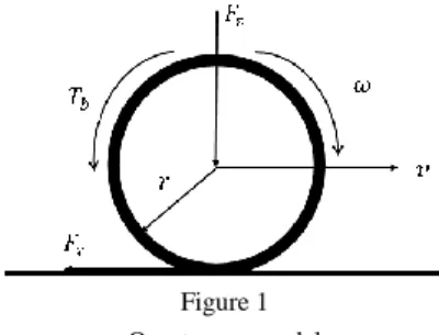
A quarter-car model is used to develop the longitudinal braking dynamics. It consists of a single wheel carrying a quarter mass m of the vehicle, and at any given time t, the vehicle is moving with a longitudinal velocity v t( ). Before brakes are applied, the wheel moves with an angular velocity of ( )t , driven by the mass m in the direction of the longitudinal motion. Due to the friction between the tyre and the road surface, a tractive force Fx is generated. When the driver applies the braking torque, it will cause the wheel to decelerate until it comes to a stop. A two degree of freedom quarter-car model is shown in Figure 1.
Figure 1 Quarter-car model
Applying Newton’s second law of motion, the equations describing the vehicle, tyre and road interaction dynamics during braking are given by Equations (1) and (2).
The equation describing the wheel rotational dynamics is given by:
1 r ( )Fz B T signb( ( ))
J (1)
where is the angular velocity of the wheel, J is the rotational inertia of the wheel, r is the radius of the tyre, B is the viscous friction coefficient of the wheel bearings and Tb is the effective braking torque, which is dependent on the direction of the angular velocity.
The equation describing the vehicle longitudinal dynamics is given by:
1 2
( ) z
v F Cv
m
(2)
where v is the longitudinal velocity of the vehicle, C is the vehicle’s aerodynamic friction coefficient, is the longitudinal friction coefficient between the tyre and the road surface is the longitudinal tyre slip and Fz is the normal force exerted on the wheel.
The hydraulic brake actuator dynamics is modelled as a first-order system given by:
1
b b b b
T T k P
(3)
where kb is the braking gain, which is a function of the brake radius, brake pad friction coefficient, brake temperature and the number of pads [21], and Pb is the braking pressure from the action of the brake pedal which is converted to torque by the gain kb. The hydraulic time constant accounts for the brake cylinder’s filling and dumping of the brake fluid [21].
2.2 Friction Model
The friction coefficient between the road and the tyre has a significant influence on the braking or traction of the vehicle. The wheel slip results in the deformation and sliding of tread elements in the tyre/road patch. A simple definition of the longitudinal slip () is given by:
v r v
(4)
The frictional forces developed between the tyre and the road surface is a complex non-linear problem, which attracted a lot of research work in the eighties to nineties [22, 23, 24, 25]. When the rotation of the wheel around its axle is free, partly or fully locked, three phenomena are likely to take place; these are free
rolling, skidding and full locking. The available maximum acceleration / deceleration of the vehicle body is determined by the maximum friction coefficient describing the contact of the road and the wheels. For this reason, the behaviours of various tyres under various environmental conditions are extensively studied [22, 25, 26, 27, 28]. The physics involved in the modeling of the rolling phenomenon is complex. Bakker et al. [22] in the late eighties and Zanten et al. [29] in the early nineties concentrated on clarifying the role of the so called “wheel slip” parameter, which is defined by Equation (4). The wheel slip was found to be a critical parameter on which the available maximal friction coefficient depends [30], also shown in Figure 2. A parameter essentially identical to this wheel slip is found to be crucial by measurements [31]. However, a practically useful model need not be so complex. The development of a practical friction model may enhance the performance of the ABS controller.
Figure 2
Curves for different road conditions
Equation (4) has a physical deficiency because of the normalization with v. In the definition of
,
no dependence on the absolute value of v is taken into account, though the relative velocity of the skidding surfaces is determined by v r . Most friction models like the magic formulae [22] are affected by this physical deficiency. The Burckhardt's model given by Equation (5) on the other hand contains the relative velocity of the car body to road, v.
2
41 3
( , ) 1 C C v
x v C e C e
(5)
where:
C1 is the maximum value of the friction curve C2 is the friction curve shape
C3 is the friction curve difference between the maximum value and the value at
1
C4 is the wetness characteristics, which are in the range 0.02C40.04s m
This formulae was evidently developed for v0( cannot be defined for v0) and for r
0,v . Since and v are physically independent variables, different possible /v ratios may occur in practice. For example, the v0 situation may happen while 0 that makes indefinite. Besides this problem, it can be observed that the indefinite quantities may appear in the exponent of the approximating functions in the model. In order to eliminate these numerical difficulties, which could make the results of numerical situations unreliable, the present work has adopted a static tyre-road friction model proposed by [32] given as:0
0 2 2
0
( ) 2
(6)
in which 0 can be interpreted as the “optimal slip ratio” and 0 denotes the available maximum of the friction coefficient. This model has the advantage that it gives a good result when , and its sign modification can also be physically interpreted as turning from braking to accelerating phase, and vice versa. However, it also has the special property that for v r 0 (i.e. for rolling without skidding) it yields 0. Therefore, it can describe the case of locked wheels when v0.
3 Controller Design
3.1 Input-Output Feedback Linearization
In the input-output feedback linearization method, the output y is differentiated r times to generate an explicit relationship between the output and the input. For any controllable system of order n, it will require at most n differentiations of the output for the control input to appear. This implies that rn, where r is referred to as the relative degree of the system. If the control input never appears, the system is uncontrollable or undefined. If on the other hand rn, there will be internal dynamics, which cannot be seen from the external input-output relationship. Depending on whether the internal dynamics are stable or unstable, further transformation of the states and analysis is required. The internal dynamics are usually difficult to analyse, and hence the zero dynamics are often analysed instead [33, 34]. For a well-defined system (i.e. rn), a controller is designed to cancel the non-linearity. For an undefined or uncontrollable system, it is not possible to linearise the system. The current work is based on a well-defined relative degree as will be shown later.
In addition, the feedback linearization control approach is applicable to a class of non-linear systems described by the canonical form given by Equation (7) [35].
( ) ( )
f g u
x x x (7)
( )
yhx (8)
where the state variables x
x x1, 2
Tare the wheel angular velocity and the vehicle longitudinal velocity v respectively, f g, :R® R are smooth functions and y is the output slip function. It will be shown that the ABS problem is a single input single output (SISO) affine non-linear system of the form represented by Equation (7).The wheel slip dynamics is obtained by taking the derivative of the longitudinal wheel slip (Equation 4) with respect to time, assuming that the radius of the tyre remains constant.
d dv d dr
dt v dt dt r dt
(9)
2
r r
v v v
(10)
Substituting (1) and (2) into (10) yields the following:
2
x b x
rF T F
r r
v J v m
(11)
Rearranging (11) and knowing that FxFz
, 0
yields the slip dynamics as2
0
1 r z( , ) r b
F T
v mv J Jv
(12)
The slip dynamics represented by Equation (12) resembles Equation (7) where
2
0
( ) 1 r z( , ), ( ) r
f x F g x
v mv J Jv
and uTb. In this case, f( )and ( )
g are nonlinear dynamic functions. The goal of the ABS is to track a predetermined slip set-point (d). At this operating point, it is safely assumed that g x( )0, and hence the control input can be chosen as:
1 ( )
u ( ) f x
g x
(13)
where is a virtual input.
The nonlinearity in (12) is therefore cancelled and a simplified relationship between the integral of the output and the new input can be presented as:
(14)
The wheel slip control is an output tracking problem. The objective is to find a control action u t( ) that will ensure the plant follows the desired slip trajectory within acceptable boundaries, keeping all the states variables and controllers bounded. On this basis, the following assumptions are necessary [36]:
Assumption 1
The vehicle velocity v and wheel speed are measurable or observable.
Assumption 2
The desired trajectory vector defined within a compact subset of Rl, ld( )t Î Ud, is assumed to be continuous, available for measurement, and ld( )t £ Wx with
Wx as a known bound.
Let the tracking error ( )e be given as:
( ) d( )
e t t (15)
and let the new input be chosen as:
d e
(16)
where is a positive constant. From (13) and (14), the closed-loop tracking error dynamics will be:
0
ee (17)
3.2 Stability Analysis
Even though the control input (16) is shown to provide perfect tracking, as shown by (17), it is desirable to show that the system is stable in the Lyapunov sense.
If the new input is defined as:
( 1)
1 n ... ( 1) ...
v e n e xnd
(18) where the design parameters v and s are chosen heuristically [37], and is the filtered error signal given by:
1 2
1 1
1 2 ...
n n
n n n
d e d e
e
dt dt
(19)
Taking the derivative of will yield:
v (20)
Considering the following Lyapunov function:
1 2
V 2 (21)
the derivative of (21) will yield:
( 1) ( 2)
1 ( 1)
( 1) ( 2) ...
n n
n n n
d e d e
V e
dt dt
(22)
It can be seen that e0 exponentially as 0over time, while the design parameters 1... n1 are chosen so that the system is stable. For example, if before braking e(0)e(0)0, then e t( ) 0 t 0; this signifies perfect tracking of the slip.
4 Proposed Wheel Slip Controller Scheme
The current work proposes a hybrid system that combines feedback linearization (FBL) and PID controllers to realise the hybrid FBLPID controller. The FBLPID hybrid solution for the ABS takes advantage of the FBL approach, in which a non- linear system is transformed into a linear system [38, 34]. This makes it possible to apply a linear PID controller instead of the traditional pole placement controller. The problem identified with the FBL method incorporating pole placement approach for the ABS is that it inherently chatters. Since the linear controller realised from the input-output feedback linearization scheme already contains proportional and derivative terms of the error signal, the proposed scheme therefore adds an integral term to handle the chattering of the braking torque. The arrangement of the proposed hybrid system is shown in Figure 3, and the governing equation for the PID controller used in the hybrid system is given by Equation 23.
Figure 3
Hybrid FBLPID slip controller structure
1 1
( ) ( )
1
i d
p
i d
T s T s
U s K E s
T s T s
(23)
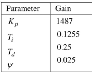
The Simulink® optimization toolbox incorporating a gradient descent search method is used to choose the gains for the PID controller. The gains are presented in Table 1
Table 1 PID gains for hybrid system
Parameter Gain Kp
Ti
Td
1487 0.1255 0.25 0.025
5 Simulation Results and Discussions
In order to evaluate the performance of the proposed controllers, three performance indices are adopted. These are: the integral squared error [ISE] of the slip 2
0 tf
d dt
, the integral squared control input 20 tf
T dtb
, and the stopping distance0 tf
vdt [40]. The desired performance will therefore be: small variations from the desired slip, less effective braking torque, to achieve a shorter stopping distance.Simulations are conducted on a straight-line braking operation, braking commenced at an initial longitudinal velocity of 80km h, and the braking torque was limited to 1200Nm. In order to impose a desired slip trajectory, the following reference model is adopted [41].
( ) 10 ( ) 10 ( )
d t d t c t
(24)
where the slip command is chosen to be c 0.18.
The parameters and numerical values used are presented in Table 2.
Table 2
System parameters and numerical values
Symbol Description Value Unit
m Quarter-car mass 395 kg
J Moment of Inertia 1.6 2
/ Nms rad
r Radius of wheel 0.3 m
C Vehicle viscous friction 0.856 kg m/
B Wheel viscous friction 0.08 2
/ N kg m s
Hydraulic time constant 0.3 s
b Hydraulic gain 0.8 Constant
g Gravitational acceleration 9.81 m s/ 2
d Desired slip 0.18 Ratio
Simulations are conducted for high and low friction surfaces with friction coefficients of 0.85 and 0.2, respectively. These friction coefficients correspond to dry asphalt and icy road conditions, respectively [42]. The simulations are terminated at speeds of about 4km h. This is because as the speed of the wheel approaches zero, the slip becomes unstable, therefore the ABS should disengage at low speeds to allow the vehicle to come to a stop.
Simulation results for the vehicle and wheel deceleration for both FBL and FBLPID controllers are shown in Figures 4 to 7 for high and low friction road conditions. The vehicle deceleration is represented by dash-lines while the wheel angular deceleration is represented by a continuous line. Figures 8 to 11 gives the slip tracking plots the desired slip is shown in dash-lines and the tracking slip is shown as continuous line. It can be observed that in some cases the difference between the slip tracking and the desired slip is not obvious; this is a case of perfect tracking. The braking torque simulation results are presented in Figures 12 to 15 for both the standard FBL controller and the proposed hybrid controller, respectively. The summarised performance results are presented in Tables 3 and 4.
The primary objective for developing the hybrid system is to solve the chattering effect observed in the FBL controller performance by enhancing the FBL controller with a PID controller to smooth-out the control action. The proposed hybrid controller achieves stopping distances of 29m and 103mon high and low friction road conditions, respectively. This yields a 6% improvement on the high friction road and 19% improvement on the low friction road when compared to the standard FBL controller.
Figure 4 Figure 5
Vehicle & wheel deceleration using FBL Vehicle & wheel deceleration using FBLPID
controller with 0.85 controller with 0.85
Figure 6 Figure 7
Vehicle & wheel deceleration using FBL Vehicle & wheel deceleration using FBLPID
controller with 0.2 controller with 0.2
Table 3
Simulation results for 0.85road condition
Performance index Specs. FBL Proposed-FBL
Integral square error min 65.99 0.2113
Integral square input Nm2 105 min 2.411 2.083
Stopping distance
m 50 31 29Figure 8 Figure 9
Slip tracking using FBL with 0.85 Slip tracking using FBLPID with 0.85
Figure 10 Figure 11
Slip tracking using FBL with 0.2 Slip tracking using FBLPID with 0.2
Table 4
Simulation results for 0.2road condition
Performance index Specs. FBL Proposed-FBL
Integral square error min 1.412 4.148
Integral square input Nm2 105 min 0.645 0.481
Stopping distance
m 50 127 103Figure 12 Figure 13
Braking torque using FBL with 0.85 Braking torque using FBLPID with 0.85
Figure 14 Figure 15
Braking torque using FBL with 0.2 Braking torque using FBLPID with 0.2 The hybrid system equally utilises less effective braking torques when compared to the maximum allowable torque. It recorded an effective braking torque of 1135Nm on the high friction road, which is about 1% higher than the standard FBL, and 267Nmon the low friction road, about 1.5% above that of the standard FBL. Comparing the plots of the hybrid system in Figures 13 and 15 to those of the standard FBL in Figures 12 and 14, chattering has been reduced considerably.
The slightly higher braking torques utilised by the hybrid system is compensated for by the reduced chattering. The effective braking torques plots showed a high initial torque values at the on-set of the braking on all road conditions, but this phenomenon is more pronounced on the low friction road condition. Taking this situation into consideration, therefore, the hybrid controller out-performs the standard FBL as revealed on the effective braking torque performance index in Tables 3 and 4.
The slip tracking plots for the hybrid system are shown in Figures 9 and 11. The hybrid system exhibits a slight unstable slip situation towards the end of the simulation for the high friction road condition. It gives, however, almost perfect slip tracking on the low friction road condition. The hybrid system records lower performance index values than the FBL with respect to slip tracking, as indicated in Tables 3 and 4.
Conclusion and Future Work
This paper proposes a hybrid feedback linearization method in combination with a PID controller for solving the chattering problem observed in the application of the standard feedback linearization to the ABS control problem. The over-all performance of the proposed method demonstrates a superior performance over the standard FBL controller for the ABS. Correlating the plots with the performance results presented in Tables 3 and 4 confirms this assertion. The robustness of both controllers, however, can be seen in their performances at low friction road conditions, where both the transient and steady state conditions of the slip behaved quite well, thereby avoiding excessive slippage.
The scope of this paper covers vehicle dynamics modeling, controller design and analysis and implementation in simulations using the Matlab® / Simulink® simulation environment. Future work will investigate the application of intelligent-based FBL control scheme.
References
[1] Solyom S.: Control of Systems with Limited Capacity, PhD Thesis, Lund Institute of Technoogy, 2004
[2] Petersen I.: Wheel Slip Control in ABS Brakes Using Gain Scheduled Optimal Control with Constrians, PhD Thesis, Norwegian University of Science and Technology, Norway, 2003
[3] Wellstead P., Pettit N.: Analysis and Re-Designof an Antilock Brake System Controller, IEE Proceedings on Control Theory and Applications, Vol. 144, No. 5, pp. 413-426
[4] Aly A. A, Zeidan E. S., Hamed A., Salem F.: An Antilock-Braking System (ABS) Control: A Technical Review, Intlligent Control and Automation, August 2011, Vol. 2, pp. 186-195
[5] Yoo D.: Model-based Slip Control via Constrained Optimal Algorithm, Master’s thesis, RMIT University, 2006
[6] John S., Pedro J., Pozna C.: Enhanced Slip Control Performance Using Nonlinear Passive Suspension System, Proceedings of the IEEE/ASME International Conference on Advanced Intelligent Mechatronics, Hungary, 2011, pp. 277-282
[7] Jiang F., Gao Z.: An Application of Nonlinear PID Control to a Class of Truck ABS Problems, Proceedings of the 40th IEEE Conference on Decision and Control Vol. 1, 2001, pp. 516-521
[8] O’Dwyer A. Handbook of PI and PID Controller Tuning Rules, 3rd Edition, Imperial College Press, 2009
[9] Panagopoulos H, Astrom K. J.: PID Control Design and H∞ loop Shapping, International Journal of Robust and Nonlinear Control, 2000, Vol. 10, No.
15, pp. 1249-1261
[10] Austin L., Morrey D.: Recent Advances in Antilock Braking Systems and Traction Control Systems, Proceedings of the Institute of Mechanical Engineers, Part D: Journal of Automobile Engineering, January 2000, Vol.
214, No. 6, pp. 625-638
[11] Buckholtz K. R. Reference Input Wheel Slip Tracking Using Sliding Mode Control, SAE Technical Series, 2002
[12] Jing Y., Mao Y., Dimirovski G, Zheng S.: Adaptive Global Sliding Mode Control Strategy for the Vehicle Antilock Braking Systems, Proceedings of the American Control Conference, 2009, pp. 769-773
[13] Lu H. C.: Grey Prediction Approach for Designing Grey Sliding Mode Controller, Proceedings of IEEE International Conference on Systems, Man and Cybernetics, Vol. 1, 2004, pp. 403-408
[14] Li J., Yibo Z., Haipeng P., Chattering-Free Grey Sliding Mode Control for Discrete Time-Delay Systems with Unmatched Uncertainty, Proceedings of the 3rd International Conference on Intelligent System and Knowledge Engineering, Vol. 1, 2008, pp. 983-986
[15] Kayacan E., Oniz Y., Kaynak O. A., A Grey System Modeling Approach for Sliding-Mode Control of Antilock Braking System, IEEE Transactions on Industrial Electronics, August 2009, Vol. 56, No. 8, pp. 3244-3252 [16] Oniz Y., Kayacan E., Kaynak O., Simulated and Experiemtal Study of
Antilock Braking System Using Grey Sliding Mode Control, IEEE International Conference on Systems, Man and Cybernetics, 2007, pp. 90- 95
[17] Jun C.: The Study of ABS Control System with Different Control Methods, Proceedings of the 4th International Symposium on Adavced Vehicle Control, Nagoya Japan, 1998
[18] Assdian F.: Mixed H∞ and Fuzzy Logic Controllers for the Automobile ABS, SAE Technical Series, March 2001
[19] Park K. S., Lim J. T., Wheel Slip Control for ABS with Time Delay Input Using Feedback Linearization and Adaptive Sliding Mode Control, Proceedings of the International Conference on Control, Automation and Systems, 2008, pp. 290-295
[20] Shin H. S., Choi H. L., Lim J. T.: Feedback Linearization of Uncertain Nonlinear Systems with Time Delay, IEE Proceedings on Control Theory and Applications November 2006, Vol. 153, No. 6, pp. 732-736
[21] Alleyne A.: Improved Vehicle Performance Using Combined Suspension and Braking Forces, Vehicle Systems Dynamics, International Journal of Vehicle Mechanics and Mobility, 1997, Vol. 27, No. 4, pp. 235-265 [22] Bakker E., Pacejka H., Lidner L.: A New Tire Model with an Application
in Vehicle Dynamics Studies, SAE Technical Seires, 1998, pp. 83-95 [23] Pacejka H., Bakker E.: The Magic Formula Tyre Model, Proceedings of the
1st International Colloquium on Tyre Models for Vehicle Dynamics Analysis, 1993, Vol. 21, pp. 1-18
[24] Oosten J. V., Bakker E.: Determination of Magic Tyre Model Parameters, Proceedings of 1st International Colloquium on Tyre Models for Vehicle Dynamics Analysis, 1993, Vol. 21, pp. 19-29
[25] Linder L.: Experience with the Magic Formula Tyre Model, 1st International Colloquium on Tyre Models for Vehicle Dynamics Analysis, 1993, Vol. 21, pp. 30-46
[26] Canudas-de Wit C., Tsiotras P.: Dynamic Tire Friction Friction Models for Vehicle Traction Control, Proceedings of the 38th IEEE Conference on Decision and Control, Vol. 4, 1999, pp. 3746-3751
[27] Lacombe J.: Tire Model for Simulations of Vehicle Motion on High and Low Friction Road Surfaces, Simulation Conference Proceedings, Vol. 1, 2000, pp. 1025-1034
[28] Olson B. J.: Nonlinear Dynamics of Longitudinal Ground Vehicle Traction, Master’s Thesis, Michigan State University, 2001
[29] Zantn A, Erhardt R., Lutz A.: Measurement and Simulation of Transients in Longitudinal and Lateral Tire Forces, SAE Technical Series, 1990, pp. 300- 318
[30] Corno M., Savaresi S. M., Balas G. J.: On Linear-Parameter-Varying (LPV) Slip-Control Design for Two-wheeled Vehicles, International Journal of Robust and Nonlinear Control, 2009, Vol. 19, No. 12, pp. 1313- 1336
[31] Yagi K., Kyogoku K., Nakahara T.: Relationship between Temperature Distribution in EHL Film and Dimple Formation, Journal of Tribology, 2005, Vol. 127, No. 3, pp. 658-665
[32] Lin J. S., Ting W. E.: Nonlinear Control Design of Anti-Lock Braking Systems with Assistance of Active Suspension, Control Theory Applications IET, January 2007, Vol. 1, No. 1, pp. 343-348
[33] Slotine J. J., Li W.: Applied Nonlinear Control, Printice-Hall, New Jersey, USA, 1991
[34] Hedrick J, Girard A, Feedback linearization, 2005
[35] Ball S., Barany E., Schaffer S., Wedeward K.: Nonlinear Control of Power Network Models Using Feedback Linearization, Proceedings of the Circuits, Signals and Systems, Oklobdzija, 2005, pp. 493-800
[36] Yesildrirek A., Lewis F.L.: Adaptive Feedback Linearization Using Efficient Neural Networks, Journal of Intelligent and Robotics Systems, May 2001, Vol. 31, pp. 253-281
[37] Behera L., Kar I.: Intelligent Systems and Control: Principles and Applications, Oxford University Press, 2009
[38] Henson M. A, Seborg D.E.: Nonlinear Process Control, Prentice-Hall, 1997 [39] Zhang D., Chen Y., Xie J., Ai W., Yuan C.: A Hybrid Control Method of Sliding Mode and PID Controllers Based on Adaptive Controlled Switching Portion, Proceedings of the 29th Control Conference 2010, pp.
439-445
[40] Mirzaeinejad H., Mirzaei M.: Anovel Method for Non-Linear Control of Wheel Slip in Anti-Lock Braking Systems, Control Engineering Practice, 2010, Vol. 18, No. 8, pp. 918-926
[41] Poursamad A.: Adaptive Feedback Linearization Control of Antilock Braking Systems Using Neural Networks, Mechatronics, 2009, Vol. 19, No. 5, pp. 767-773
[42] MacIsaac Jr J. D., Garrot W. R.: Preliminary Findings of the Effect of Tire Inflation Pressure on the Peak and Slide Coefficients of Friction, Technical Report, National Highway Traffic Safety Administration, Washington D.C., 20590, USA, 2002