Preliminary Moho depth determination from receiver function analysis using AlpArray stations in Hungary

(1)

ORIGINAL STUDY

Preliminary Moho depth determination from receiver function analysis using AlpArray stations in Hungary

Dániel Kalmár^1,2 · Bálint Süle² · István Bondár² · the AlpArray Working Group

Received: 21 September 2017 / Accepted: 3 May 2018 / Published online: 14 May 2018

Abstract Receiver function analysis is applied to the western part of the Pannonian Basin, a rather complex region both geologically and geodynamically. Previous receiver function analyses in this region had to deal with much smaller station density and time span than those available to us. In the analysis we used the data of some 48 seismological stations. These include not only the permanent stations from Hungary and permanent stations from neighbouring countries (Slovakia and Slovenia), but also the temporary broadband stations that were installed within the framework of the AlpArray project. Hav- ing applied rather strict manual quality control on the calculated radial receiver functions we stacked the receiver functions. Using the H–K grid search method we determined the Moho depth and the Vp/Vs ratio beneath the seismological stations in the western part of the Pannonian Basin. The unprecedented density of the AlpArray network, combined with the permanent stations, allowed us to derive high resolution Moho and Vp/Vs maps for the West Pannonian Basin, together with uncertainty estimates. Our preliminary results agree well with previous studies and complement them with finer details on the Moho topography and crustal thickness.

Keywords Pannonian Basin · AlpArray project · Receiver function analysis · Moho discontinuity

* Dániel Kalmár

kalmardani222@gmail.com

1 Department of Geophysics and Space Science, Institute of Geography and Earth Sciences, Eötvös Loránd University, Budapest, Hungary

2 Kövesligethy Radó Seismological Observatory, Geodetic and Geophysical Institute, Research Centre for Astronomy and Earth Sciences, Hungarian Academy of Sciences (MTA CSFK GGI KRSZO), Budapest, Hungary

(2)

1 Introduction

Our region of interest was the western part of the Pannonian Basin and the easternmost part of the Eastern Alps. The Pannonian Basin is a geologically complex extensional back- arc basin in Central Europe (Horváth et al. 2006). It is characterized by compression stress fields and left strike-slip movements (Fodor 2010). The Eastern Alps has similar evolution history to the Pannonian Basin (Schmid et al. 2008). The region shows medium seismic activity due to the advance of the Adriatic microplate. The Vienna Basin has similar sediment thickness as the Pannonian Basin but unlike the Pannonian Basin, the Mur-Mürz- Zilina zone is a seismically very active area (Horváth et al. 2006).

The receiver function method is based on the notion that teleseismic waveforms contain information that can be used to determine the crustal and upper mantel characteristics of the Earth underneath seismic stations (Ammon 1991). In this paper, we applied receiver function analysis to determine the depth of the crust-mantle boundary under the West Pan- nonian Basin.

The first crustal thickness map of the Carpathian-Pannonian region was composed by Horváth (1993) by using the available national maps mostly based on reflection seismic measurements. Lenkey (1999) modified the map by making compatible the seismically obtained pattern with the gravitational anomalies of the basin. Taking into account of new deep seismic profiles and results of gravitational modelling studies Horváth et al. (2006) improved a new Moho map. The most recent version of this map is published by Horváth et al. (2015).

Receiver functions were analysed by Hetényi and Bus (2007) at four permanent stations in Hungary. In case of two stations the obtained Moho depth agreed very well with the map of Horváth et al. (2006), at the other two ones receiver function analysis indicates about 5 km thicker crust.

Grad et al. (2009) compiled the first digital, high-resolution map of Moho for the whole European Plate from individual seismic profiles, body and surface wave tomography studies, receiver function results and maps of seismic and gravity data compilations.

Recently the crustal structure of the region studied in this paper was investigated by applying ambient noise tomography by Ren et al. (2013) and by receiver functions analysis by Hetényi et al. (2015). These studies used the data of the Carpathian Basin Project array which comprised three lines of broadband seismometers and covered a 75 km wide zone across the western Pannonian Basin.

Thanks to the AlpArray project the station density and time span we could use in this study is much larger. The AlpArray project is a European initiative, with the aim to advance our understanding of orogenesis and its relationship to mantle dynamics, surface processes and seismic hazard in the Alps–Apennines–Carpathians–Dinarides orogenic system. We calculated receiver functions and determined depth of Moho beneath 13 permanent stations and 29 temporary AlpArray stations.

2 Data

The AlpArray seismic network provides uniform coverage of the greater Alpine area with seismometers deployed at unprecedented density. This presents 220 permanent and 350 temporary AlpArray seismological broadband stations (Hetényi et al. 2018). The waveform

(3)

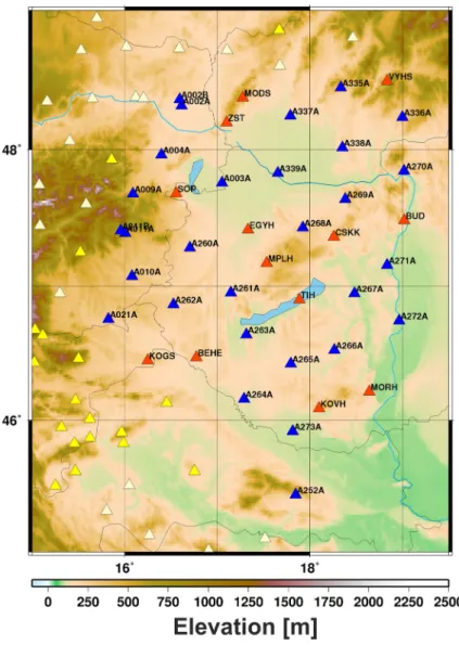
data are available for participants of the project, at the ORFEUS EIDA node (European Integrated Data Archive). The Hungarian component of this network consists of 14 broadband stations in addition to the 9 permanent stations of the Hungarian National Seismo- logical Network (HNSN) (Gráczer et al. 2018). The experiment has officially started on January 1, 2016. Thus, besides data from the HNSN and the Hungarian component of the AlpArray temporary deployment, we used 10-month worth of data from 15 stations of the AlpArray temporary network and 4 permanent stations from neighbouring countries (Slovakia and Slovenia). As for the HNSN broadband stations we used all available data from the start date of their operations up until October 31, 2016. Figure 1 shows the 13

Fig. 1 The map shows the seismic network in the West Pannonian Basin. The red triangles represent permanent stations and the blue triangles represent temporary AlpArray stations. The yellow and white triangles show the non-Hungarian permanent and temporary AlpArray stations that were not used in this study

(4)

permanent stations and 29 temporary AlpArray stations we used for the receiver function analysis.

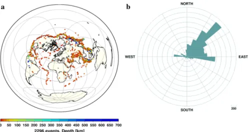
For the receiver function analysis we considered waveforms from teleseismic earthquakes between 25° and 96° epicentral distances and magnitudes larger than 5.5. The selection of events is expected to provide reasonable signal to noise ratio. Note that we extended the upper bound of epicentral distances from 90° to 96° so that we can get bet- ter azimuthal coverage by including events along the west coast of Central and Northern America. Figure 2a shows the selected events. Figure 2b shows the back azimuthal coverage indicating that the vast majority of earthquakes occurred in the Himalayas, the Indo- nesian archipelago and Japan. We downloaded the broadband three-component waveforms from the HNSN and ORFEUS-EIDA servers.

To determine the time window of the waveforms to be downloaded we used the reported irst P arrivals in the Hungarian National Seismological Bulletin (HNSB) for the Hungarian stations (Gráczer et al. 2004–2015). At the non-Hungarian temporary AlpArray stations we did not use HNSB, because the reviewed bulletin for 2016 was not yet available. Therefore in this case we used predicted first P wave arrivals using the ak135 (Kennett et al. 1995) travel time tables.

3 Receiver function analysis

The basis of the method is that incident P waves generated from teleseismic events are con- verted to S wave (Ps) and other multiples (PpPs and PpSs + PsPs) at discontinuities associ- ated with large seismic velocity contrast such as the Moho discontinuity. We used broadband 3-component seismograms for the P receiver function analysis. The procedure rotates the ZNE components into the ZRT coordinate system and performs the deconvolution by dividing Fourier transforms of the R and T components by the Fourier transform of the Z component. The computed receiver functions represent the relative response of the Earth structure below the stations without source and station effects. In other words, the receiver

Fig. 2 a The map shows the 2296 earthquakes that were used in the receiver function analysis. b Most of the earthquakes occurred in the Himalayas, the Indonesian archipelago and Japan

(5)

functions approximate the Green’s function of the local structure beneath a seismic station (Grad and Tiira 2012). We applied the frequency-domain deconvolution method for the receiver function analysis in this study (Ammon 1997).

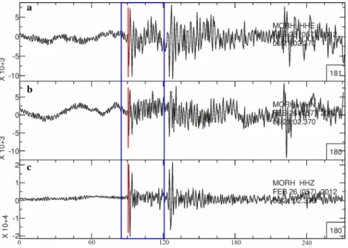
We used a 35 s time-window, with 5 s lead and 30 s lag times. Because the crustal thickness below the Pannonian Basin is shallower than below the Alps and Carpathians, the 35 s time-window will include the major multiples from the Moho interface. In most cases this relatively short time-window contains useful signals with good signal-to-noise ratio (Fig. 3).

After the removal of the mean and trend, the waveforms were filtered with a But- terworth band-pass filter between 0.033 and 1 Hz (Hetényi et al. 2015). During the pre-processing of waveforms, the Seismic Analysis Code (SAC, Goldstein et al. 2003), and the General Seismic Application Computing (GSAC, Herrmann 2013) were used.

For receiver function analysis the pwaveqn (Ammon 1997) software is applied. The pwaveqn software rotates the seismograms from the ZNE system to the ZRT coord- ianate system and performs the deconvolution in frequency-domain. This deconvolution method strongly depends on the water-level and Gauss-filter parameters. The water- level parameter avoids division by zero by adding a small value to the denominator. The Gauss-filter removes high-frequency noise in the receiver functions, this in fact impacts the maximum amplitude of the receiver functions. The water-level and the Gaussian- filter are required parameters that were determined by trial-and-error by testing a range of values. We set the water-level and Gauss-filter values to 0.01 and 1.5, respectively.

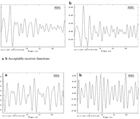
Because of the relative instability of the frequency domain deconvolution (Ammon 1997) we performed manual quality control of the radial receiver functions (Figs. 4, 5).

This step represented the most time consuming process, but it was quite important to

Fig. 3 E, N and Z waveform components from the 2012-02-26 Taiwan earthquake recorded at MORH. The red line shows the first P arrival time. The blue lines present the start and end of a 35 s time-window

(6)

select receiver functions with the best quality. We accepted only those receiver functions where both the first-arriving P and the first multiple, Ps could be clearly seen, otherwise we rejected the receiver function. Figure 4 illustrates cases of accepted and Fig. 5 shows rejected receiver functions.

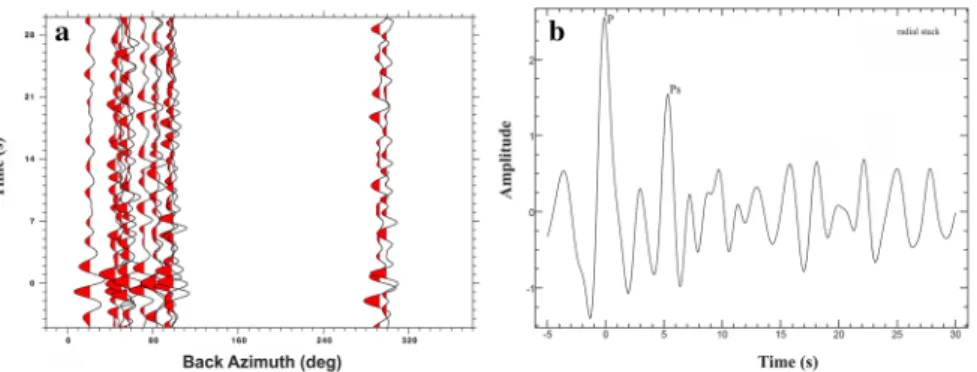
After the quality control process we grouped and stacked the receiver functions by back-azimuth. We grouped the receiver functions into 36, 10 degree-wide back- azimuth bins. We stacked the receiver functions in each group to increase signal-to- noise ratio for the receiver function. This grouping allowed us to investigate if there is a significant azimuthal dependence in the receiver functions. In most cases there was not, which allowed us using the full, azimuthally independent stack in our analysis. Finally, we obtained the full-stack receiver function when we stacked the receiver functions of the back-azimuth groups. Figure 6 shows an example for this stacking procedure.

The stacked receiver functions formed the input for the H–K grid search method (Helffrich et al. 2013), where H represents the Moho depth and K stands for the Vp/

Vs ratio. We set the Vp to 5.8 km/s, which is the average P velocity in the crust of the Pannonian Basin (Gráczer and Wéber 2012). We set the limits in H–K analysis for the Moho depth between 20 and 40 km and for the Vp/Vs ratio between 1.5 and 2. These values represent physically meaningful limits for the Pannonian Basin. We manually checked the H–K results (Crotwell and Owens 2005) by inspecting the absolute and local Fig. 4 a, b Acceptable receiver functions

Fig. 5 a, b The rejected receiver functions

(7)

maxima. We selected the physically most meaningful maximum, which was not neces- sarily the absolute maximum. Figure 7 shows an example of the H–K analysis at BEHE.

4 Results

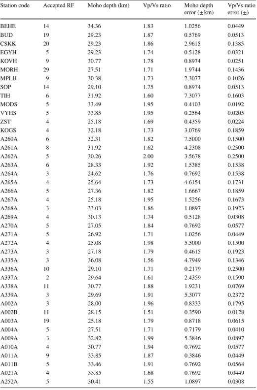
We present Moho depth values and Vp/Vs ratios under the investigated stations we used in this study. Table 1 shows the results of the H–K grid search for each station.

Since the permanent stations in Hungary had longer operating periods than the rest of the stations, they produced more accepted receiver functions than the other (AlpArray and non-Hungarian permanent) stations. We only had 10-month worth of data at the AlpAr- ray and non-Hungarian permanent stations, therefore the number of receiver functions that passed the manual review is inevitably smaller. Figure 8 shows the events with accepted receiver functions and the azimuthal coverage of receiver functions. Similar to the original distribution of the selected events shown in Fig. 2, most accepted receiver functions obtained from events from the Himalayas, the Indonesian archipelago and Japan.

Figure 9a shows the Moho map obtained from the receiver function analysis for the western part of the Pannonian Basin. We focused on the West Pannonian Basin because Fig. 6 a Receiver functions ordered by back-azimuth at BEHE station. b The full-stack receiver function at BEHE

Fig. 7 Results of the H–K Grid search method at the BEHE seismological station

(8)

Table 1 The table summarizes the results

Station code Accepted RF Moho depth (km) Vp/Vs ratio Moho depth

error (± km) Vp/Vs ratio error (±)

BEHE 14 34.36 1.83 1.0256 0.0449

BUD 19 29.23 1.87 0.5769 0.0513

CSKK 20 29.23 1.86 2.9615 0.1385

EGYH 5 29.23 1.74 0.5128 0.0321

KOVH 9 30.77 1.78 0.8974 0.0251

MORH 29 27.51 1.71 1.9744 0.1436

MPLH 9 30.38 1.73 2.3077 0.1026

SOP 14 29.10 1.75 0.8974 0.0513

TIH 6 31.92 1.60 7.3077 0.1603

MODS 5 33.49 1.95 0.4103 0.0192

VYHS 5 33.85 1.95 0.2564 0.0205

ZST 4 25.18 1.69 0.4359 0.0224

KOGS 4 32.18 1.73 3.0769 0.1859

A260A 6 32.31 1.82 7.5000 0.1500

A261A 8 31.92 1.62 4.2308 0.2500

A262A 5 30.26 2.00 3.5678 0.2500

A263A 6 28.33 1.92 1.5385 0.1538

A264A 3 24.62 1.76 0.7692 0.1538

A265A 4 25.64 1.73 4.6154 0.1731

A266A 5 27.36 1.82 1.6667 0.1859

A267A 4 25.18 1.95 1.5256 0.1673

A268A 3 33.03 1.86 1.0897 0.1923

A269A 4 30.13 1.74 0.5128 0.0308

A270A 5 27.05 1.84 0.7692 0.0577

A271A 5 26.92 1.71 1.0256 0.0449

A272A 4 25.08 1.98 5.5000 0.1500

A273A 3 27.18 1.79 0.4615 0.1923

A335A 3 36.08 1.56 4.7949 0.1346

A336A 10 29.10 1.71 0.2179 0.2500

A337A 2 29.64 1.61 2.4359 0.1590

A338A 11 30.77 1.88 1.9231 0.0769

A339A 3 29.69 1.91 5.3077 0.2372

A002A 3 28.00 1.96 0.8333 0.1795

A002B 11 28.15 1.51 0.3590 0.0128

A003A 19 25.18 1.79 0.8718 0.0615

A004A 5 27.51 1.71 0.7179 0.0410

A009A 3 32.82 1.99 5.3846 0.0897

A010A 4 30.77 1.94 0.7692 0.0577

A011A 9 33.85 1.87 0.3846 0.0449

A011B 5 33.46 1.91 0.7692 0.0564

A021A 4 33.85 1.68 0.7692 0.0449

A252A 5 30.41 1.55 1.0897 0.0308

The columns present the station code, the number of accepted receiver functions, the Moho depth, the Vp/

Vs ratio, the Moho-depth errors and the Vp/Vs errors

(9)

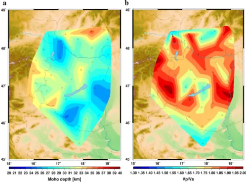
there we could obtain the best resolution for the Moho map owing to the station density of the AlpArray network. Hence, we ignored the stations in the eastern part of the Pan- nonian. The Moho depth values change between 24 and 36 km. The Mid-Hungarian

Fig. 8 a The map presents the 409 events with accepted receiver functions. b Back azimuthal coverage of accepted receiver functions

Fig. 9 Maps present the Moho depth (a) and Vp/Vs ratios (b) in the western part of the Pannonian Basin from the receiver function analysis

(10)

Zone and Little Hungarian Plain is characterised by thinner crust (24–28 km), while by the foothills of the Alps, Carpathians and Transdanubian Mountains indicate larger crustal thickness (30–33 km). These results are in good agreement with previous studies and complement them with finer details in the Moho topography (Grad et al. 2009;

Hetényi et al. 2007, 2015; Lenkey 1999; Horváth et al. 2015).

Figure 9b shows the Vp/Vs ratio map for the western part of the Pannonian Basin.

The calculated Vp/Vs values in every case change between 1.5 and 2 in the western part of the Pannonian Basin. We obtained somewhat higher values (1.8–2) for the studied area. Recall that we used 5.8 km/s Vp velocity for every station, which is the average crustal P velocity in the Pannonian Basin (Gráczer and Wéber 2012). However, we admit that this value may not always be the best estimate in the Eastern Alps and the Carpathians. Similarly, the choice of the 35 s time-window might be too short for the surrounding orogenic regions, but for our focus area this choice is acceptable.

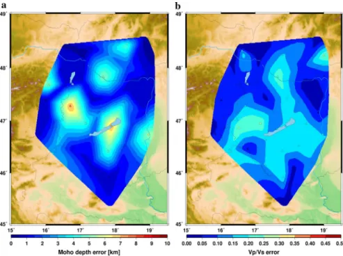
Figure 10 shows the uncertainties in the Moho depth and Vp/Vs ratio obtained from the H–K grid search. In most cases, the Moho depth uncertainty is about one km. We obtain somewhat larger (4–7 km) values at BSZH, CSKK, TIH and A260A because the multiples were not very well defined in the full stack receiver function. The Vp/Vs ratio uncertainties vary between 0.05 and 0.25, with the majority of the errors around ± 0.1.

Fig. 10 The maps present a the Moho depth and b the Vp/Vs ratio errors for western part of the Pannonian Basin obtained from the H–K analysis

(11)

5 Discussions and conclusions

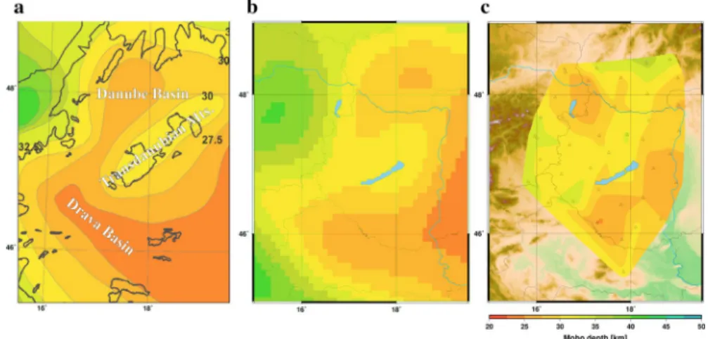
Figure 11 show three Moho maps. The leftmost is the latest published Moho map of the West Pannonian Basin (Horváth et al. 2015), the middle one is published by Grad et al.

(2009) from seismic profiles, body and surface wave tomography and receiver function analysis and finally the rightmost one is our map. For the sake of comparison, the three maps are presented in the same colour scale and step interval. The comparison of the three Moho maps indicates that owing to the higher resolution provided by the AlpAr- ray network, in most cases our results are able to resolve more subtle changes of the Moho discontinuity than the map of Horváth et al. (2015) and Grad et al. (2009).

We can identify shallower crust in the Danube Basin and in the surrounding areas, as well as in the central part of Hungary and Drava Basin. The shallow crust of (25–27 km) in the Danube Basin agrees well with Hetényi et al. (2015) and can also be found on the Horváth et al. (2015) map, while it is not present in the Grad et al. (2009) map. The crustal thickness (20–25 km) below the Drava Basin shows the largest discrepancies, most likely because of the lack of reliable data.

The Transdanubian Mountains exhibits somewhat thicker crust (30–33 km) and is in a good agreement whith Grad et al. (2009), Horváth et al. (2015) as well as Ren et al.

(2013) and Hetényi et al. (2015). Our map also indicates thicker crust below the Car- pathians than the maps of Horváth et al. (2015) and Grad et al. (2009). All maps show thicker crust in the Alps than in the Pannonian Basin.

We conclude that our preliminary results, obtained purely from P-receiver function analysis, correlate well with previous studies and complement them with finer details in the Moho topography and crustal thickness. The unprecedented density of the AlpAr- ray network, combined with the permanent stations, allowed us to derive high resolution Moho and Vp/Vs maps for the West Pannonian Basin, together with uncertainty estimates. However, during the manual quality control of the receiver functions we had to reject a large number of receiver functions because of the relative instability of the frequency domain deconvolution method. Therefore, in the follow up of this effort where we compute not only radial P receiver functions, but also S receiver functions and investigate anisotropy using both radial and transverse receiver functions, we will use

Fig. 11 Comparison of the Moho maps from a Horváth et al. (2015), b Grad et al. (2009), c from this study

(12)

the more stable, but slower iterative time-domain deconvolution (Ligorría and Ammon 1999).

Acknowledgements The reported investigation was supported by the National Research, Development and Innovation Fund (No. K124241). Waveforms were used from the AlpArray temporary network (https ://doi.org/10.12686 /alpar ray/z3_2015), from the Hungarian National Seismological Network (https ://doi.

org/10.14470 /uh028 726), the Slovak National Seismological Network (https ://doi.org/10.14470 /fx099 882) as well as the Slovenian National Seismological Network (https ://doi.org/10.7914/sn/sl). We would like to thank to the authors of Generic Mapping Tools (GMT) software (Wessel and Smith 1998). The authors thank the two anonymous reviewers whose comments helped to improve the paper.

References

Ammon CJ (1991) The isolation of receiver effects from teleseismic P waveforms. Bull Seismol Soc Am 81:2504–2510

Ammon CJ (1997) An overview of receiver function analysis. http://eqsei s.geosc .psu.edu/~cammo n/HTML/

RftnD ocs/rftn0 1.html Accessed 22 Apr 2017

Crotwell HP, Owens JT (2005) Automated receiver function processing. Bull Seismol Soc Am 76:702–709 Fodor LI (2010) Mezozoos-kainozoos feszültségmezők és törésrendszerek a Pannon-medence ÉNy-i

részén—módszertan és szerkezeti elemzés. DSc thesis, Budapest

Goldstein PD, Dodge M, Firpo LM (2003) SAC2000: signal processing and analysis tools for seismologists and engineer. IASPEI Int Handb Earthq Eng Seismol 81:1613–1620

Gráczer Z, Wéber Z (2012) One-dimensional P-wave velocity model for the territory of Hungary from local earthquake data. Acta Geodaetica et Geophysica Hungarica 473:344–357

Gráczer Z, Bondár I, Czanik C, Czifra T, Győri E, Kiszely M, Mónus P, Süle B, Szanyi G, Tóth L, Varga P, Wesztergom V, Wéber Z (2004–2015) Hungarian National Seismological Bulletin. http://www.seism ology .hu/index .php/en/seism icity /earth quake -bulle tins. Accessed 08 May 2017

Gráczer Z, Szanyi G, Bondár I, Czanik C, Czifra T, Győri E, Hetényi G, Kovács I, Molinari I, Süle B, Szűcs E, Wesztergom V, Wéber Z, AlpArray Working Group (2018) AlpArray in Hungary: temporary and permanent seismological networks in the transition zone between the Eastern Alps and the Pannonian basin. Acta Geodaetica et Geophysica Hungarica. https ://doi.org/10.1007/s4032 8-018-0213-4 Grad M, Tiira T (2012) Moho depth of the European Plate from teleseismic receiver functions. J Seismol

16:95–105

Grad M, Tiira T, ESC Moho Working Group (2009) The Moho depth of the European plate. Geophys J Int 176:279–292

Helffrich G, Wookey J, Bastow I (2013) The seismic analysis code: a primer and user’s guide. Cambridge University Press, Cambridge

Herrmann RB (2013) Computer programs in seismology: an evolving tool for instruction and research. Seis- mol Res Lett 84:1081–1088. https ://doi.org/10.1785/02201 10096

Hetényi G, Bus Z (2007) Shear wave velocity and crustal thickness in the Pannonian Basin from receiver function inversions at four permanent stations in Hungary. J Seismol 11:405–414

Hetényi G, Ren Y, Dando B, Stuart GW, Hegedűs E, Kovács AC, Houseman GA (2015) Crustal structure of the Pannonian Basin: the Alcapa and Tisza terrains and the mid-Hungarian zone. Tectonophysics 646:106–116

Hetényi G, Molinari I, Clinton J, Bokelmann G, Bondár I, Crawford WC, Dessa JX, Doubre C, Friederich W, Fuchs F, Giardini D, Gráczer Z, Handy MR, Herak M, Jia Y, Kissling E, Kopp H, Korn M, Margh- eriti L, Meier T, Mucciarelli M, Paul A, Pesaresi D, Piromallo C, Plenefisch T, Plomerová J, Ritter J, Rümpker G, Sipka V, Spallarossa D, Thomas C, Tilmann F, Wassermann J, Weber M, Wéber Z, Wesz- tergom V, Zivcic M, Team ASN, Crew AOC, Group AW (2018) The AlpArray seismic network—a large-scale European experiment to image the Alpine orogeny. Surv Geophys. https ://doi.org/10.1007/

s1071 2-018-9472-4

Horváth F (1993) Towards a mechanical model for the formation of the Pannonian Basin. Tectonophysics 226:333–357

Horváth F, Bada G, Windhoffer G, Csontos L, Dombrádi E, Dövényi P, Fodor L, Grenercy G, Síkhegyi F, Szafián P, Székely B, Tímár G, Tóth L, Tóth T (2006) A Pannon-medence jelenkori geodinamikájának atlasza: Euro-konform térképsorozat és magyarázó. Magyar Geofizika 47:133–137

(13)

Horváth F, Musitz B, Balázs A, Végh A, Uhrin A, Nádor A, Koroknai B, Pap N, Tóth T, Wórum G (2015) Evolution of the Pannonian basin and its geothermal resources. Geothermics 53:328–352

Kennett BLN, Engdahl ER, Buland R (1995) Constraints on seismic velocities in the Earth from traveltimes.

Geophys J Int 122:108–124

Lenkey L (1999) Geothermics of the Pannonian basin and its bearing on the tectonics of basin evolution.

PhD thesis, Vrije Universiteit Amsterdam

Ligorría JP, Ammon CJ (1999) Iterative deconvolution and receiver-function estimation. Bull Seismol Soc Am 89:1395–1400

Ren Y, Grecu B, Stuart G, Houseman G, Hegedüs E, South Carpathian Project Working Group (2013) Crustal structures of the Carpathian–Pannonian region from ambient noise tomography. Geophys J Int 195:1351–11369. https ://doi.org/10.1093/gji/ggt31 6

Schmid SM, Bernoulli D, Fügenschuh B, Matenco LC, Schefer S, Schuster R, Tischler M, Ustaszewski K (2008) The Alpine-Carpathian-Dinaridic orogenic system: correlation and evolution of tectonic units.

Swiss J Geosci 101:139–183

Wessel P, Smith WHF (1998) New, improved version of the Generic Mapping Tools Released. EOS Transcr Am Geophys Union 79:579