Live electronics
Szigetvári Andrea
Siska Ádám
Live electronics
Szigetvári Andrea Siska Ádám
Copyright © 2013 Andrea Szigetvári, Ádám Siska
iii
Table of Contents
Foreword ... x
1. Introduction to Live Electronics ... 1
2. Fixed-Media and Interactive Systems ... 3
1. Studio Tools ... 3
1.1. Sequencers ... 3
1.2. DAWs and Samplers ... 3
1.3. Integrated Systems ... 3
1.4. Composing in the Studio ... 4
2. Interactive Systems ... 4
2.1. Roles of Interactive Systems ... 4
2.2. Composition and Performance Issues ... 6
3. Description of Live Electronic Pieces ... 7
1. Karlheinz Stockhausen: Mantra (1970) ... 7
1.1. Gestures Controlling the System and Their Interpretation ... 7
1.2. Sound Processing Unit ... 8
1.3. Mapping ... 8
1.4. The Role of Electronics ... 8
2. Andrea Szigetvári: CT (2010) ... 9
2.1. Gestures Controlling the System ... 11
2.2. Gesture Capture and Analysis Strategies ... 12
2.3. Sound Synthesis and Processing Unit ... 12
2.4. Mapping ... 13
4. Listing and Description of Different Types of Sensors ... 16
1. Defining Controllers ... 16
2. Augmented Instruments ... 16
3. Instrument-like Controllers ... 18
4. Instrument-inspired Controllers ... 21
5. Alternate Controllers ... 24
5. Structure and Functioning of Integra Live ... 30
1. History ... 30
2. The Concept of Integra Live ... 31
2.1. Structure of the Arrange View ... 31
2.2. Structure of the Live View ... 33
3. Examples ... 35
4. Exercises ... 37
6. Structure and Functioning of Max ... 39
1. History ... 39
2. The Concept of Max ... 39
2.1. Data Types ... 40
2.2. Structuring Patches ... 41
2.3. Common Interface Elements and Object Categories ... 41
2.4. Mapping and Signal Routing ... 43
3. Examples ... 43
3.1. Basic Operations ... 44
3.2. Embedding ... 45
3.3. Signal Routing ... 45
3.4. Data Mapping ... 46
3.5. Templates ... 47
4. Exercises ... 49
7. OSC - An Advanced Protocol in Real-Time Communication ... 50
1. Theoretical Background ... 50
1.1. The OSC Protocol ... 50
1.2. IP-based Networks ... 50
2. Examples ... 51
3. Exercises ... 53
8. Pitch, Spectrum and Onset Detection ... 55
1. Theoretical Background ... 55
1.1. Signal and Control Data ... 55
1.2. Detecting Low-Level Parameters ... 55
1.3. Detecting High-Level Parameters ... 56
1.3.1. Pattern Matching ... 56
1.3.2. Spectral Analysis ... 56
1.3.3. Automated Score Following ... 56
2. Examples ... 56
2.1. Analysis in Integra Live ... 56
2.2. Analysis in Max ... 57
3. Exercises ... 60
9. Capturing Sounds, Soundfile Playback and Live Sampling. Looping, Transposition and Time Stretch 62 1. Theoretical Background ... 62
1.1. Methods of Sampling and Playback ... 62
1.2. Transposition and Time Stretch ... 63
2. Examples ... 63
2.1. Sampling in Integra Live ... 64
2.2. Sampling in Max ... 64
3. Exercises ... 66
10. Traditional Modulation Techniques ... 68
1. Theoretical Background ... 68
1.1. Amplitude and Ring Modulation ... 68
1.2. Frequency Modulation ... 69
1.3. The Timbre of Modulated Sounds ... 70
2. Examples ... 71
2.1. Ring Modulation in Integra Live ... 71
2.2. Modulation in Max ... 72
3. Exercises ... 74
11. Granular Synthesis ... 76
1. Theoretical Background ... 76
2. Examples ... 76
2.1. Granular Synthesis in Integra Live ... 77
2.2. Granular Synthesis in Max ... 78
3. Exercises ... 79
12. Sound Processing by Filtering and Distortion ... 81
1. Theoretical Background ... 81
1.1. Filtering ... 81
1.2. Distortion ... 82
1.2.1. Harmonic and Intermodulation Distortion ... 82
1.2.2. Quantization Distortion ... 83
2. Examples ... 83
2.1. Filtering and Distorting in Integra Live ... 84
2.2. Filtering and Distorting in Max ... 85
3. Exercises ... 89
13. Sound Processing by Delay, Reverb and Material Simulation ... 91
1. Theoretical Background ... 91
1.1. Delay ... 91
1.2. Reverberation ... 91
1.3. Material Simulation ... 92
2. Examples ... 92
2.1. Material Simulation in Integra Live ... 92
2.2. Delay and Reverb in Max ... 92
3. Exercises ... 93
14. Panning, Surround and Multichannel Sound Projection ... 95
1. Theoretical Background ... 95
1.1. Simple Stereo and Quadro Panning ... 95
1.2. Simple Surround Systems ... 95
1.3. Multichannel Projection ... 95
1.4. Musical Importance ... 96
v
2. Examples ... 96
2.1. Spatialisation in Integra Live ... 96
2.2. Spatialisation in Max ... 97
3. Exercises ... 98
15. Mapping Performance Gestures ... 99
1. Theoretical Background ... 99
1.1. Mapping ... 99
1.2. Scaling ... 99
2. Examples ... 100
2.1. Mappings in Integra Live ... 100
2.2. Mappings in Max ... 101
3. Exercises ... 103
16. Bibliography ... 104
List of Figures
2.1. On the one hand, the number and type of data structures that control sound processing and synthesis are defined by the gesture capture strategies, the analysis, and the interpretation of control data. On the other hand, the number of (changeable) parameters of the sound-producing algorithms is fixed by the algorithms themselves. Mapping creates the balance between these by specifying which control data belongs to which synthesis parameter, as well as the registers to be controlled. The choice of feedback
modalities influences the way how the performer is informed about the results of their gestures. ... 5
3.1. Process of the CT scan of metal wires: a) Position of the wire in the computer tomograph. The red lines indicate 2 intersections. b) 2 frames created by the intersection: 1th section contains one, the 2nd section contains three 'sparks'. c) The final results are bright shining sparks projected on a black backgound. ... 9
3.2. Slices of the original video of 2,394 frames (100 sec). ... 10
3.3. The score of CT, derived from the five identified orbits. These are displayed as horizontal lines, the one below the other. For each line, those frames where the respective orbit is active are marked red; inactive parts are coloured black. ... 12
3.4. The structure of the sound engine of a single voice, showing the avaliable synthesis and processing techniques (soundfile playback, granular synthesis, subtractive synthesis and distortion), together with their controllable parameters and the possible routes between the sound generating units. ... 12
3.5. The parameters of the sound engine which are exposed to the dynamic control system based on the motion of the sparks. ... 13
3.6. The matrix controlling the mappings within a single voice. The red dots specify the synthesis parameters that are assigned to the individual control data in a certain preset. The green number boxes set the ranges of the incoming control data, while the red ones define the allowed ranges for the controlled parameters. ... 14
4.1. Yamaha Disklavier. ... 16
4.2. Serpentine Bassoon, a hybrid instrument inspired by the serpent. Designed and built by Garry Greenwood and Joanne Cannon. ... 17
4.3. MIDI master keyboards of different octave ranges. In fact, most master keyboards also contain a set of built-in alternate controllers, like dials and sliders. ... 18
4.4. Electronic string controllers: violin (left) and chello (right). ... 19
4.5. The Moog Etherwave Theremin ... 21
4.6. Two different laser harp implementations which both send controller values for further processing. The LightHarp (left), developed by Garry Greenwood, uses 32 infrared sensors to detect when a 'virtual string' is being touched. As the 'strings' are infrared, they can not be seen by humans. The laser harp (right), developed by Andrea Szigetvári and János Wieser, operates with coloured laser beams. ... 22
4.7. The Hands, developed by Michel Waisvisz. An alternate MIDI controller from as early as 1984. 24 4.8. Reactable, developed at the Pompeu Fabra University. The interface recognises specially designed objects that can be placed on the table and executes the 'patches' designed this way. ... 26
4.9. The Radio Baton (left) and its designer, Max Matthews (right). ... 27
4.10. Kinect, by Microsoft. ... 28
5.1. A Tap Delay Module and its controls. ... 31
5.2. A Stereo Granular Synthesizer Module and its controls. ... 32
5.3. A Block containing a spectral delay. ... 32
5.4. An example project containing three simultaneous Tracks. A few Blocks contain controllers controlled by envelopes. ... 33
5.5. Routings between different elements and external (MIDI CC) data sources. ... 33
5.6. The most relevant controllers of each Track, as shown in the Live View. ... 34
5.7. Three Scenes in the timeline of Integra Live. ... 34
5.8. The 'virtual keyboard' of the Live View, showing the shortcuts of Scenes. ... 34
5.9. The sound file player. Click on the 'Load File' field to load a sound file. Click on the 'Bang' to start playing it. ... 35
5.10. The keyboard shortcuts associated with the Scenes of the demo project. ... 35
5.11. The main switch between the Arrange and Live Views. Also depicted are the playback controls (top left) and the button (in blue) that would return us from the Module View to the Block View. ... 36
5.12. The demo project, in Arrange View. We may see all the involved Envelopes and Scenes. .... 36
5.13. The first Block of Track1, under Module View. The Properties Panel displays the controls of the test tone Module. ... 37
vii
5.14. The first Block of Track2. Top: Module View. Bottom: Live View. ... 37
6.1. Most common objects for direct user interaction. ... 42
6.2. The application LEApp_06_01. Subpatches open by clicking on their boxes. ... 43
6.3. The basics subpatch, containing four tiny examples illustrating the basic behaviour of a few Max objects. ... 44
6.4. The embedding subpatch, showing different implementations of the same linear scaling method. 45 6.5. The routing subpatch, containing an Analog-to-Digital-Converter (ADC) input, a file player and two synthetic sounds that may be routed to the left and right loudspeakers. ... 46
6.6. The mapping subpatch, showing several examples of linear and non-linear scalings. ... 46
6.7. The templates subpatch, showing the different templates used through these chapters. ... 48
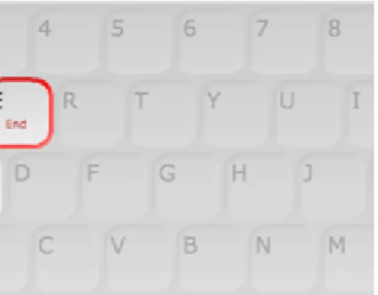
6.8. Generic keyboard input. ... 48
7.1. Find out the IP addresses of your network interfaces. ... 51
7.2. A synthesizer, consisting of three independent modules, which can be controlled via OSC. .... 51
7.3. An OSC-based synthesizer contol interface. ... 53
8.1. An oscillator controlled by low-level musical parameters extracted from an input signal. ... 57
8.2. The spectrum and sonogram of an incoming signal. ... 57
8.3. Simple spectral analysis tools in Max. ... 58
8.4. A MIDI-driven rhythmic pattern matcher in Max. ... 59
8.5. A MIDI-driven melodic pattern matcher in Max. ... 59
9.1. A sampler with individual control over transposition and playback speed. ... 64
9.2. A simple sampler presenting both hard drive- and memory-based sampling techniques. The current setting gives an example of circular recording and looped play-back of the same buffer: while recording into the second half of the buffer, the first part of the same buffer is being played back. ... 64
9.3. A 4-channel hard disk-based circular recording and play-back engine in Max. All channels use separate playback settings, including the possibility of turning them on and off individually. Sound files are created and saved automatically. ... 65
9.4. A harmoniser in use. The current setting, adding both subharmonic and harmonic components, adds brightness while transposes down the input signal's base pitch by several octaves. ... 66
10.1. Spectrum of Ring (a) and Amplitude (b) Modulation. ... 68
10.2. Frequency Modulation. ... 69
10.3. FM spectrum. ... 69
10.4. Ring modulation in Integra Live: the most important controls of the ring modulator. ... 71
10.5. Ring modulation in Integra Live: the test tone and file player sources. ... 71
10.6. Amplitude and Ring modulation in Max. ... 72
10.7. Simple FM in Max. ... 73
10.8. Infinitely cascaded frequency modulation by means of feedback. ... 73
11.1. A granular synthesizer in Live View. It can process either pre-recorded sounds (stored in Granular.loadsound) or live input (which can be recorded with Granular.recSound). ... 77
11.2. The same granular synthesizer, this time with parameters controlled by envelopes. ... 77
11.3. A simple granular synthesizer in Max with live-sampling capabilities. ... 78
12.1. The spectra of an incoming signal and a filter's response to it. ... 81
12.2. Idealised amplitude responses of several filter types. Upper row (from left to right): LP, HP, BP, BR; lower row (from left to right): LS, HS, AP. fc stands either for cutoff-frequency or centre-frequency; b stands for bandwidth. The AP response depicts the phase response as well, to illustrate the role of these filters. ... 81
12.3. Hard clipping (right) applied to a pure sine wave (left). The red lines indicate the threshold. 82 12.4. Illustration of poor quantization (red) of a pure sine wave (black). ... 83
12.5. The le_12_01_integra.integra project in Integra Live. ... 84
12.6. Overdrive (soft and hard clipping) in Integra Live. ... 84
12.7. LEApp_12_01. ... 86
12.8. LEApp_12_02. ... 86
12.9. Hard clipping in Max. ... 87
12.10. Quantization distortion in Max. ... 88
12.11. LEApp_12_04: an instrument built entirely on filtering and distorting short bursts of noise. 88 13.1. Material simulation in Integra Live. ... 92
13.2. A simple delay line in Max. ... 93
13.3. A simple cascaded reverberator in Max. Every reverberator (whose number is set by the 'Number of reverbs') obtains the same values. ... 93
14.1. Stereo panning in Integra Live. ... 96
14.2. Quadraphonic panning in Integra Live. ... 96
14.3. A simple stereo panner in Max. The 2D interface controls both the stereo positioning and depth. 97 14.4. Ambisonics-based 8-channel projection in Max, using up to four individual monophonic sources. 98 15.1. A block consisting of a test tone, modulated, filtered and distorted in several ways. ... 100
15.2. Routings of Block1. ... 100
15.3. Routings of Block2. ... 100
15.4. A basic (but complete) interactive system in Max. ... 101
ix
List of Tables
2.1. The phases of interactive processing proposed by three different authors. One can observe that, as time progresses, the workflow becomes more exact and pragmatic (thanks to cumulative experience).
4
6.1. List of the most common objects for direct user interaction. ... 41
Foreword
This syllabus approaches the realm of real-time electronic music by presenting some of its most important concepts and their realisations on two different software platforms: Integra Live and Max.
Both applications are built on the concept of patching, or graphical programming. Patches contain small program modules - called unit generators - which can be connected together. Unit generators are 'black boxes' whose internal logic is hidden from the musicians, performing some well-defined, characteristic action. The behaviour of the patch as a whole depends on the choice of unit generators and the connections that the musician creates between them.
The visual design of Integra Live resembles a more traditional multitrack sequencer, with multiple tracks and a timeline. The main novelty of the software is that, instead of containing pre-recorded samples, the tracks contain patches. In other words, rather than holding actual sounds, each track describes processes to make sounds, extending the philosophy of the traditional sequencer towards live, interactive music performance.
Max, on the other hand, offers no more than a blank canvas to its user. Although this approach requires a more computer-oriented way of thinking, it does not put any borders in the way of the musicians' imagination.
Chapter 1-4 present the basic aspects of live electronic music, pointing out the typical differences (in terms of aesthetics, possibilities and technical solutions) between tape music and live performance. To illustrate these, analyses of two pieces involving live electronics is presented. A detailed description of sensors used by performers of live electronic music is also included.
Chapters 5-6 introduce the two software environements used in this syllabus, Integra Live and Max, respectively.
Chapter 7 describes protocols that allow different pieces of software and hardware (including sensors) to communicate with each other in a standardised way.
Chapter 8 defines and presents different methods to capture low- and high-level musical descriptors in real-time.
These are essential in order to let the computer react to live music in an interactive way.
Chapters 9-11 describe different methods of creating sounds. Some of these are based on synthesis (the creation of a signal based on a priori principles), others on capturing existing sounds, while others mix these two approaches.
Chapters 12-13 contain techniques of altering our sound samples by different sound processing methods.
Chapter 14 is centred on the issues of sound projection.
Chapter 15 introduces the quite complex problematics of mapping, focusing on the questions of transforming raw sensor data into musically meaningful information.
Every Chapter starts with an introduction, describing the purpose, basic behaviour and possible parameters (and their meanings) of the methods presented. This is followed by examples realised in Integra Live and Max (some Chapters do not contain Integra Live examples). The purpose of these examples is demonstration, emphasizing simple control and transparency; indeed, they cannot (and are not intended to) compete with commercially available professional tools. Moreover, in some cases, they deliberately allow some settings and possibilities that professional tools normally forbid by design. Our goal in this was a better illustration of the nature of some techniques through the exploration of their extreme parameters and settings.
The syllabus contains a number of excercises, to facilitate understanding through practice of the principles and methods explored.
To run the example projects for Integra Live, Integra Live needs to be downloaded and installed (available freely from http://www.integralive.org under the GPL license). Software written in Max were converted into standalone applications - there is no need to have a copy of Max in order to open these files.
1
Chapter 1. Introduction to Live Electronics
The first electroacoustic works - not considering pieces using electro-mechanic instruments, like the ondes Martenot - were realized for fixed media (in most cases, magnetic tape). Performing such music consists of playing back the recordings, the only human interaction being the act of starting the sound flow.
The reason behind this practice was purely practical: the realization of these works required the use of devices, which at the time were available only in a few 'experimental' studios. In addition, the time scale of preparing the sound materials was many orders of magnitude above the time scale of the actual pieces. This made it impossible to create these works in real-time. As an example, the realization of Stockhausen's Kontakte, a key piece in the history of early electroacoustic music, took almost two years between 1958 and 1960.
Preparing music in a studio has its own benefits. Besides avoiding the inevitable errors of a live performance, the composer is able to control the details of the music to a degree that is not achievable in a real-time situation:
in a studio, it is possible to listen each sound as many times as needed, while experimenting with the different settings of the sound generator and manipulating devices. The composer can compare the results with earlier ones after each modification and make tiny adjustments to the settings when needed. These are perhaps the key reasons why many composers, even today, choose to create pieces for fixed media. However, tape music has raised a number of issues since its birth.
Within a decade of the opening of the first electronic studios, many composers realized the limitations inherent in studio-made music. For most audiences, the presence of a performer on stage is an organic element of the concert situation. Concerts presenting pre-rendered music feature only a set of loudspeakers distributed around the venue. While the soundscape created by such performances may indeed be astonishing, the lack of any human presence on stage challenges the listener's ability to sustain focused attention.
Another issue arises from the questions of interpretation and improvisation, which are, by their nature, 'incompatible' with the concept of fixed media. Moreover, not only is tape-improvisation impossible, but subtle in situ adjustments, which are so natural in traditional music practice - for example, the automatic adaptation of accompanying musicians to a soloist or the tiny adjustment of tuning and metre to the acoustics of the performance hall - are excluded as well. This problem manifests itself when mixing tape music with live instruments, and becomes much more apparent when the music has to co-exist with other art forms, like dance.
This latter was perhaps the main reason that pushed composers like John Cage towards methods which could be realized in 'real-time', leading to such early productions as Variations V (1965), composed for the Cunningham Dance Company.
As a consequence of the above (and many other) arguments, the demand for the possibility of performing electronic music under 'real-time' circumstances increased over time, eventually giving birth to the world of 'live' electronic music.
Although the first works of this genre were already created in the mid-sixties, it was not until the millenium that the idea of live performance in electronic music became widespread1. Moreover, most works involving live electronics were themselves experimental pieces, where improvisation played a great role. The lack of proper recordings as well as documentation (both musical and technical) makes the researchers' task very hard; a detailed summary of the history of the first decades of live electronic music is still awaited2.
What changed the situation during the past (two) decade(s)?
The obvious answer is the speed and capacity of modern computers, which have played an undisputable role in the evolution of live-performed electronic music. Unlike the studio equipment of the eighties, the personal computer offers an affordable solution for many musicians to use as (or create) musical devices which fit their aesthetic needs.
1As a landmark: one of the most important conferences on the subject, New Interfaces for Musical Expression (NIME) was first held in 2001.
2And, as the 'protagonists' of that era - the only sources we could rely on - pass away, such summary might never materialise.
However, this is not the only reason. Computers just do what their users tell them to do: without proper software solutions and knowledge, even super-fast computers are not much help. The development of software paradigms with live performance in mind - either based on pre-existing studio paradigms, or on completely new ideas - have also made a great impact on the genre. These new paradigms allow musicians to discuss their ideas, creating communities with an increased amount of 'shared knowledge'. This knowledge boosts interest in live electronic music (both from the prespective of musicians and researchers) and serves as inspiration for many artists engaging with the genre.
3
Chapter 2. Fixed-Media and Interactive Systems
Since the advent of fast personal computers, the performance practice of electroacoustic music has been in continuous transformation. The emergent drive desire of live interpretation possibilities is forcing tape music to yield it's primacy to new digital interactive systems - also called Digital Music Instruments (DMI). The field is still in a pioneering, transitional state, as it is difficult to compete with the quality of both past and present acousmatic and computer music, created using non-real-time techniques. A key reason behind this is that the compositional process itself is inseparable from its realisation, allowing the careful creation of the fixed, final sound material of the piece. Therefore, developers of DMIs have to solve (at least) two essential problems:
• Invent strategies that substitute (recreate) the non real-time studio situation, where sonorities are the result of numerous sequential (consecutive, successive) procedures.
• Develop appropriate ways of gestural control to shape the complex variables of the musical process.
1. Studio Tools
To better understand the main issues of interactivity, we first present the most important devices involved in studio-based (offline) composition. These solutions have been constantly evolving during the past sixty years, and development is still active in the field, to say the least. Nonetheless, the past decades have already given us enough experience to categorise the most important instruments of non-real-time music editing.
1.1. Sequencers
A sequencer allows recording, editing and play-back of musical data. It is important to emphasize that sequencers deal with data instead of the actual sound, thus, they represent an abstract, hierarchical conceptualisation of musical information. In contrast to sound editors, a sequencer will not offer the possibility of editing the signal. Instead, the information is represented in a symbolic way. This could be a musical score, a piano roll, or any other symbolic representation. However, in contrast to traditional scores, a sequencer may display (as well as capture and/or play back) information that is not available in a 'traditional' score (for example exact amplitude envelopes, generated by MIDI controllers). As it is clear from the above, a sequencer usually contains a minor score engraver as well as the capabilities for creating and editing complete envelopes.
1.2. DAWs and Samplers
The DAW (Digital Audio Workstation) is similar to the sequencer in that it has storage, editing and play-back options. However, in contrast to a sequencer, a DAW always uses (pre-)recorded sound as a source. Thus, it is not the abstract, parametric representation of the sound that is edited, but the sonic material itself. To achieve this, a DAW usually includes a large number of plug-ins - each one capable of modifying the original sound in many different ways.
Although it was originally a separate tool, the sampler is, by now, an integral part of any DAW. A sampler stores (or, in many cases, also records) samples of original sound sources, often in high quality. Then, fed by control data arriving from (MIDI) controllers (or a sequencer), it chooses the actual sound sample to be played back, adjusting its timing, pitch, dynamics and other parameters according to the actual control values.
1.3. Integrated Systems
An integrated system is nothing more than a tool containing all listed devices. It contains a complete built-in sequencer, a DAW and a sampler. These integrated systems are usually multi-track, each track having its own inserts (plug-ins modifying the sounds of the individual tracks), notation tools that ease the creation/editing of control data in addition to actual sounds as well as extensive sample and rhythm libraries offering a broad choice of options for additional sounds. Some more advanced integrated systems offer video syncing capabilities too, allowing the creation of complex audiovisual content.
1.4. Composing in the Studio
As outlined in Chapter 1, the non-real-time composing method consists of a careful iterative process of listening, modifying and sequencing samples.
Each segment of the sound can be listened to many times, allowing the composer to concentrate on minute details of the music. According to the aesthetic needs of the piece, one can apply any combination of sound processing tools to alter the original samples. By listening to the result after each step and comparing it to the samples already created as well as the 'ideal' goal present in the imagination of the composer, one can reach any desired sound. After classifying these, one can 'build' the piece by structuring these samples in an appropriate way.
Of course, the steps outlined above are interchangeable to some extent. In many cases, composers create the temporal structure of the samples in parallel with the creation of the samples themselves. It is also possible to take abstract decisions regarding the structure in advance (based, for example, on different aesthetic or mathematical principles), long before producing the first actual sample of music.
In other words, the 'studio situation' - i.e. the opportunity of listening to and altering the samples again and again within isolated, noiseless working conditions - allows composers to create very detailed and elaborated soundscapes.
2. Interactive Systems
The offline approach, however efficient in terms of sound quality and controllability of the music, does not allow interaction with the computer, which (should be) a key element of any live performance. Hence, there has been an increasing demand for 'raising' our electronic tools to a higher musical level since the earliest days of electroacoustic music, implementing solutions that allow our devices to react to their musical environment in a (half-)automated way. Such tools are called interactive systems.
These systems are still highly individual: there are no general tools providing ready-made environments or instruments for composition. The composer/developer has to conceive their instrument from scratch, defining the musical potential of the piece to a greater extent. An established theory is also lacking: the available bibliography consists of continuously evolving reports on the actual state of developments. However, these only document some aspects of the field - mainly the tools which gradually become standardized, and can be used as building blocks for consecutive works. Reviewing the documented works, the variety of solutions is striking.
2.1. Roles of Interactive Systems
Authors writing comprehensive summaries conceptualize the workflow of interactive computer music systems in different ways. Table 2.1. outlines the main aspects of three different approaches.
Table 2.1. The phases of interactive processing proposed by three different authors. One can observe that, as time progresses, the workflow becomes more exact and pragmatic (thanks to cumulative experience).
Rowe (1993) Winkler (2001) Miranda (2006)
1. Sensing Human input, instruments Gestures to control the
system
2. Processing Computer listening Gesture capture strategies
3. Response Interpretation Sound synthesis
algorithms
4. Computer composition Mapping
5. Sound generation Feedback modalities
The stages of the classification proposed by Miranda and the relations between these is depicted in Figure 2.1.
The main elements are:
5
Figure 2.1. On the one hand, the number and type of data structures that control sound processing and synthesis are defined by the gesture capture strategies, the analysis, and the interpretation of control data. On the other hand, the number of (changeable) parameters of the sound-producing algorithms is fixed by the algorithms themselves.
Mapping creates the balance between these by specifying which control data belongs to which synthesis parameter, as well as the registers to be controlled. The choice of feedback modalities influences the way how the performer is informed about the results of their gestures.
Controlling Gestures. This means both the physical and musical gestures of the performer. When creating an interactive system, the composer/designer needs to define both the set of meaningful motions and the sonic events that may be comprehended by the machine.
Gesture Capture and Analysis. The physical gestures are captured by sensors, while sound is normally recorded by microphones. However, a gesture capture/analysis strategy is far more than just a collection of sensors and microphones: it is the internal logic which converts the raw controller and signal data into parameters that are meaningful in the context of the piece. Sensors are presented in Chapter 4 while some signal analysis strategies are explained in Chapter 8.
Sound Synthesis and Processing. This is the 'core' of an interactive system, which produces the sound. The parameters controlling the sound creation - although scaled or modified - are derived from the control values arriving from the gesture analysis subsystem.
Mapping. Normally we use a set of controllers whose values are routed in different ways to the parameters of sound synthesis. Mapping (presented in Chapter 15) denotes the way the parameters arriving from the controllers are converted into values that are meaningful for the sound generation engine.
Feedback. To have real, meaningful interaction, it is essential to give different levels of feedback to the performer simultaneously. The most obvious, fundamental form of feedback is the sound itself; however, as in the case of 'classic' chamber music (where performers have the ability to, for example, look at each other), other modes are also very important to facilitate the 'coherence' between the performer and the machine/instrument. Examples include haptic (touch-based) feedback (normally produced by the sensors themselves) or visual representation of the current internal state of the system.
2.2. Composition and Performance Issues
Compared with the tools accessible in a studio, an interactive 'performing machine' has the undisputed ability of performing live, giving musicians the ability to interpret the same piece in many different ways, as with any instrumental work. In this respect, interactive systems are much better suited for combining with 'ordinary' instruments than tape-based music. Improvisation, a realm completely inaccessible to fixed media, is made possible by these devices.
Conversely, it is much harder to achieve the same sound quality and richness with these devices compared to standard studio tools. While the offline/studio method is built on the slow process of listening to, manipulation of, editing, layering and sequencing of actual samples, an interactive system is a generic device where, during the design process, there is no way to test every possible sound generated by the instrument. Simply, the challenge for the musician wanting to work in a live, interactive, improvisational way is to begin to understand what the possibilities of real-time sound synthesis/manipulation are, given (con)temporary computational limitations.
7
Chapter 3. Description of Live Electronic Pieces
In what follows, we examine two compositions, based on the categorisation proposed by Miranda (see Chapter 2). One of these pieces (Mantra, by Karlheinz Stockhausen) was created during the very early days, while the other (CT, by Andrea Szigetvári) is a very recent piece within the genre of interactive electro(acoustic) music.
Our choice of pieces illustrates how the possibilities (both musical and technical) have evolved during the past forty years.
1. Karlheinz Stockhausen: Mantra (1970)
Mantra, a 70 minute long piece for two pianos, antique cymbals, wood blocks and live electronics was composed by Karlheinz Stockhausen (1928-2007) as his Werk Nr. 32 during the Summer of 1970 for the Donaueschinger Musiktage of the same year. It has a distinguished place within the composer's œuvre for multiple reasons. On the one hand, it is one of his first pieces using formula technique - a composition method derived by Stockhausen himself from the serial approach -, a principle which served as his main compositional method during the next 30 years, giving birth to compositions like Inori, Sirius or the 29 hour long opera Licht.
On the other hand, it was also one of his first determinate works (i.e. where the score is completely fixed) to include live electronics, and generally, his first determinate work after a long period of indeterminate compositions.
The setup requires two pianists and a sound technician. Each pianist performs with a grand piano, 12 antique cymbals, a wood block, and a special analog modulator (called 'MODUL 69 B'), designed by the composer.
Additionally, Performer I also operates a short wave radio receiver. The sound of the pianos, picked up by microphones, is routed through the modulator as well as being sent directly to the mixing desk. The combination of unprocessed and modulated piano sounds is amplified by four loudspeakers set at the back of the stage. The role of the technician is the active supervision of this mix, according to general rules set by the score.
The most comprehensible effect of MODUL 69 B is the built-in ring modulation, which is applied to the piano sound most of the time. The details of ring modulation are explained in Chapter 10. Here, we just refer to the results.
Ring modulation consists of the modulation of the amplitude of an incoming signal (called carrier) with a sine wave (called modulator). When the modulator frequency is very low (below approx. 15 Hz), the modulation adds an artificial tremolo to the timbre. With higher frequencies, two sidebands are generated per each spectral component. Depending on the ratio of the carrier and frequency, the resulting timbre may either become harmonic or inharmonic.
In the subsequent subsections, we examine the role of the ring modulation within the piece.
1.1. Gestures Controlling the System and Their Interpretation
When Stockhausen composed the piece, the choice of live controllers was very limited: the main controller of the MODUL 69 B is a simple dial (with a single output value), which controls the modulator frequency of the device. This controller allows two basic gestures:
• Rotating the dial (the output value changes continuously).
• Leaving the dial at its current position (the output value remains unaltered).
Of course, one may combine the two gestures above to create more complex ones, e.g. it is possible to rotate the dial back and forth within a range.
The dial has twelve pre-set positions, which are defined as musical tones. This representation is musically meaningful for the performer, yet it hides all irrelevant technical details from their sight. In most of the cases, the Pianists need to select one of these presets and hold them steady for very long durations. However, there are situations when they need to
• rotate the dial slowly from one preset to the other;
• play with the dial in an improvisatory way (usually, within a range defined by the score);
• vibrate the incoming sound by slowly (but periodically) altering the oscillator frequency;
• add tremolo to the incoming sound by setting the dial to very low frequency values.
The interface is quite intuitive: it is suited both for playing glissandi and for holding a steady note for as long as needed. It is consistent, as tiny changes in the dial position cause smooth and slight changes in the modulating frequency. Yet it is very simple as well: since the dials hold their position when left unattended, they require minimal supervision from both performers. Moreover, the music is composed in such a way that the performers do not need to carry out difficult instrumental passages at times when they need to control the dial.
The 'playing technique' may be learned and mastered by any musician in less than a day.
1.2. Sound Processing Unit
According to the score, MODUL 69 B consists of 2 microphone inputs with regulable amplifiers, compressors, filters, a sine-wave generator and a particularly refined ring modulator. Unfortunately, the exact internal setup is not documented (at least, in a publicly available form), which makes any discussion regarding the fine details of the device hopeless. Nevertheless, by analysing the score we may figure out that the modulation range of the ring modulator is between 5 Hz and 6 kHz. A remark by Stockhausen also clarifies that the compressor is needed in order to balance the ring-modulated piano sound, as (specially, for still sounds) the signal/noise ratio of the ring-modulated sounds differ from that of the original piano timbre.
Without knowing the internals, we can not guess the number of the device's variable parameters. It is evident that the modulator frequency is such a parameter; however, we don't know whether the built-in compressor or the filter operates with fixed values or not. While it might make sense to assume that at least one of these values (the cutoff frequency of a hypothetical high-pass filter, if there was any) would change according to the actual modulator frequency, there is no way to verify such assumptions.
1.3. Mapping
In Mantra, the dial controls the frequency of the modulator. There are twelve pre-set positions, labeled with numbers 1 to 12, corresponding to different tones of a twelve-tone row and its inverted form. However, instead of referring to these numbers, the score indicates the actual presets to use with the pitches corresponding to the particular positions.
We have no information about the particular mapping between the physical position of the dial and the corresponding frequency. However, the score suggests that the link between the position of the dial and the actual frequency is, to say the least, monotonic. Moreover, it is likely that it follows a logarithmic scaling in frequency (linear scaling in pitch), at least in the frequency region where the rows are defined (G♭3 to G♯4 for Performer I and B♯2 to C4 for Performer II).
The two basic motions, explained in Section 3.1.1., are mapped to the modulator frequency as follows:
• Changing the position of the dial causes glissandi.
• Keeping the dial position constant creates a steady modulation at a particular frequency.
1.4. The Role of Electronics
As we have said, together with the idea of representing the modulating frequencies as musical tones instead of numerical frequency values, the device is very intuitive. On the other hand, we may realise that the overall possibilities of MODUL 69 B (particularly, the expressivity allowed by the device) is very limited. We may obtain the following musical results:
• Artificial tremolo, by choosing a very low modulating frequency.
• (Timbral) vibrato, by modulating (manually) the dial around a central value.
9
• (Spectral) glissandi, by rotating the dial.
• Spectral alteration of the piano sound.
The timbral modifications introduced into the piano sound are of key importance in the piece, from both a conceptual and a musical point of view. The 'conceptual role' of the modulator frequencies is to mark the sections of the piece, which are defined by a main formula of thirteen tones (built on the previously mentioned twelve-tone row). Since the types of timbral alterations (e.g. harmonic, transposed, inharmonic etc.) of the piano sound are related to the ratio of the base pitch of the sound and the modulator frequency, having a fixed modulator frequency organizes the twelve tones into a hierarchy - defined by their relation to this modulator -, creating an abstract 'tonality'. This is different from the classical tonality, though, since octaves do not play the same role as they do in classical harmony: the results of ring modulation do change if we add an octave to an initial interval. Nevertheless, by computing - for each possible combination appearing in the piece - the timbral changes that ring modulation introduces, we could find the 'centres of gravity' of each section within the piece, underlying the role that ring modulation plays in Mantra.
2. Andrea Szigetvári: CT (2010)
CT is an audiovisual piece realised purely in Max and Jitter, applying Zsolt Gyenes' 100 second computer tomograph animation as a visual source. Computer tomography (CT) is a medical imaging technology:
normally, the scanned 'object' is the human body, for the purposes of diagnosis. To create an 'experimental' scan, metal wires were placed in the tomograph. The frames of slices of the metal wires were photographed and animated, creating unexpected results in the form of abstract moving images. The animation does not have any particular meaning, it works like a Rorschach test, where the expressive qualities, meanings are added by the viewing subjects. The music serves here as a tool to particularize the expressivity of the visual system. Different sonic interpretations of the same visual gestures are produced by an interactive music system, in which parameters are modified in real time by the performer.
Figure 3.1. shows how the cross-sections of the metal wire form the frames of a video animation.
Figure 3.1. Process of the CT scan of metal wires: a) Position of the wire in the
computer tomograph. The red lines indicate 2 intersections. b) 2 frames created by the
intersection: 1
thsection contains one, the 2
ndsection contains three 'sparks'. c) The final
results are bright shining sparks projected on a black backgound.
Figure 3.2. displays every 5th frame of a 4.2 sec long sequence of the final video. There are shiny sparks travelling in space, inhabiting different orbits, turning around, and changing their size and shape. The number of the sparks, the speed and direction of their movements varies in time.
Figure 3.2. Slices of the original video of 2,394 frames (100 sec).
11
2.1. Gestures Controlling the System
The music is controlled by the animated tomograph images. These describe five orbits, which are assigned to five musical parts. Figure 3.3. displays the activity on these orbits. This 'score' helps to indentify sections of solos, duos, trios, quartets and quintets.
Figure 3.3. The score of CT, derived from the five identified orbits. These are displayed as horizontal lines, the one below the other. For each line, those frames where the respective orbit is active are marked red; inactive parts are coloured black.
The realising software can play the 2,394 frames at different speeds:
• From the beginning to the end (original structure).
• Manually advancing frames in both directions.
• Using loops with controllable starting points, lengths and directions.
• Using random playback with controllable range and offset.
The parameters of the video playback are manipulated by the performer with a MIDI controller, which contains sliders and knobs.
As the sound sequences are controlled by the movements of the sparks of the CT animation, the gestures of the performer influence the music in an indirect way. Depending on how the video is played back, it is possible to control those movements either directly (frame by frame) or by assigning general parameters to loop or random playback.
2.2. Gesture Capture and Analysis Strategies
Each frame is represented as a set of x and y coordinates, representing the positions of the (active) sparks. An algorithm - calculating the speed of the sparks between any consecutive frames - guarantees that any combination of frames would produce a speed value, depending on how far the positions of the sparks are from each other on a given orbit.
We obtain 3 parameters per each orbit after analyzing the frames and computing the speeds. Thus, the music can be conrolled by fifteen parameters all together: x1, y1, v1, x2, y2, v2, x3, y3, v3, x4, y4, v4, x5, y5, v5.
2.3. Sound Synthesis and Processing Unit
Each orbit is linked to a different electroacoustic voice, 'sonifying' the movements of the sparks. As a result, the piece consists of five discrete (unfused) electroacoustic parts, imitating the feeling of divergent motions. The percept of different characteristics is explored by feeding similar videos to different timbre spaces.
There are 43 parameters assigned to a single voice, depicted in Figure 3.4. Together with the parameters controlling the volumes of the five voices, the low-pass filter used after their mix and the reverb (7 parameters), 43×5+5+1+7=228 parameters are available to control the sound generating engine.
Figure 3.4. The structure of the sound engine of a single voice, showing the avaliable
synthesis and processing techniques (soundfile playback, granular synthesis, subtractive
13
synthesis and distortion), together with their controllable parameters and the possible routes between the sound generating units.
2.4. Mapping
For each voice, the data received from the analysis of the video frames is mapped individually to the parameters of the sound generating engine with the help of a matrix.
As there are fewer parameters arriving from the video (15) than the total number of parameters of the sound engine (228), only a few selected musical parameters are controlled by the movements of the animation. Some parameters are kept constant, only for creating source sounds, subject to further dynamic changes. The list of dynamically changeable parameters is shown on Figure 3.5. Mapping is then reduced to the following two tasks:
1. Assigning control data to dynamically controlled parameters.
2. Defining the range of these parameters.
Figure 3.5. The parameters of the sound engine which are exposed to the dynamic
control system based on the motion of the sparks.
Figure 3.6. depicts the matrix assigned to the first voice. This matrix allows a huge number of variations: as each connection can be turned on and off individually, the connections themselves (not to mention the different scalings) offer 2(19×4)≈75558 trillion combination possibilities. The different musical motifs of the piece are created by letting the movements of the video explore different routes through the timbre space, defined by the presets of the matrices.
Figure 3.6. The matrix controlling the mappings within a single voice. The red dots
specify the synthesis parameters that are assigned to the individual control data in a
certain preset. The green number boxes set the ranges of the incoming control data,
while the red ones define the allowed ranges for the controlled parameters.
15
Chapter 4. Listing and Description of Different Types of Sensors
A controller is a device for transforming the performer's gesture into abstract machine language (in most cases, a sequence of numbers or a non-stationary electronic signal). In a live scenario, this information may either be used to control the generation, the processing or the projection of sounds (or any simultaneous combination of these). However, the data arriving from a controller is not enough per se to master these processes, as the information is normally structured in a different way than the expected parameter structure of the controlled devices. Hence, proper mappings have to be defined between the information arriving from the controllers and the parameters of the different generating, processing and projecting tools. These mappings - and the musical implications of using controllers - are explored in Chapter 15. Here, we concentrate on presenting the most commonly available controllers.
1. Defining Controllers
Historically, controllers were inherent parts of the instrument: there is no way to break an instrument into a set of controllers, synthesis/effects, and mappings between these, as the mechanical controllers are also parts of the synthesis/effect engine. In live electronic music, it is just the opposite: these independently defined entities must be merged into an instrument, giving us the freedom to use literally any human-controlled device1 to control sonic parameters. This freedom has a price, though. When 'breaking up' the instrument paradigm into these categories, we have to re-create some tasks that were automatically present in the 'composite' paradigm. Thus, in order to build a controller, one needs to define at least the following three aspects:
Communication channel. What is the means by which the controller communicates? Does it interact with the performer through physical connection? Through motion sensing?
By eye-contact? By speech recognition?
Detection. How does the device detect the above means of communication in a technical sense? Does it include buttons? Sliders? Cameras? Electrodes?
Feedback. Does the device offer any direct feedback to the performer? If yes, how is this feedback delivered?
In what follows, we present a few controllers in respect of the above issues, following a categorisation based on the conceptual distance of a controller from already existing instruments2. It must be emphasized that the borderlines between the following categories are by far not strict, though.
2. Augmented Instruments
This family consists of traditional instruments equipped with sensors. As they are built on existing instruments, the communication channel and the feedback given to the performer are defined by the base instrument. Also, even though augmented with sensors providing control data, the instrument still produces it's original sound.
A commercial product is Yamaha's Disklavier (depicted in Figure 4.1.), a real piano equipped with sensors able to record the keyboard and pedal input from the pianist. Moreover, disklaviers are equipped with appropriate tools in order to reproduce the acquired performance data. As a result, they are not only used by live electronic musicians, but also serve as tools to record, preserve and reproduce actual performances (rather than the sound of the performances) of pianists.
Figure 4.1. Yamaha Disklavier.
1Or even human-independent, like a thermometer.
2Based on E. R. Miranda and M. M. Wanderley, New Digital Musical Instruments: Control and Interaction Beyond the Keyboard (Middleton: A-R Editions, 2006).
17
Different research centres have delivered a great amount of augmented instruments during the past 30 years.
MIDI Flute, developed by IRCAM, adds sensors to the flute keys to identify the exact fingerings of the performed notes. This approach was expanded by several researchers, by adding inclination detectors or wind sensors. The Hyperinstruments (Hyperviolin, Hyperviola, Hyperchello) of MIT Media Lab combine bow motion and finger placement detection with spectral analysis of the recorded sound to provide detailed real-time performance parameters. Augmented trumpets of Princeton Media Lab include, above key pressure detectors, air-pressure sensors (microphones) built into the mouthpiece of the instrument.
Hybrids form an interesting subcategory. These are instruments that, although based on traditional instruments equipped with sensors, they no longer produce their sound in the way the original instrument does. An example is the Serpentine Bassoon (see Figure 4.2.), which is based on a classic serpent and is played with a conventional bassoon reed. However, its sound is produced electronically: it has a built-in microphone recording the acoustic sound produced by the instrument, which - after being processed by a computer - is delivered to the audience by means of electronic amplification.
Figure 4.2. Serpentine Bassoon, a hybrid instrument inspired by the serpent. Designed
and built by Garry Greenwood and Joanne Cannon.
3. Instrument-like Controllers
These devices may be imagined as if we took the 'control mechanism' out of an instrument, and possibly extending the performance possibilities (like adding additional octaves to the playable range). The reason for creating such controllers is twofold. Firstly, as most trained musicians play on acoustic instruments, a great number of potential performers may be reached with controllers that imitate the behaviour of the instruments they have already learned. Secondly, these performers already know how to master their instruments, bringing the opportunity of using advanced playing techniques in live electronic music.
Based on the construction, it is obvious that their communication channel is practically identical to the respective instrument's original set of gestures. However, the direct feedback of the controller normally lacks some of the feedback mechanisms present in the original instrument. This may be due to the lack of body vibrations (which is caused by the lack of direct sound emission) or by differences in the underlying mechanical solutions (like the different mechanisms implemented by a real piano and an electronic keyboard).
The by far most widespread such controller is the (piano-like) keyboard (see Figure 4.3.). To highlight its importance, one should consider that early modular synthesizers - like the ones manufactured by Moog or ARP - were driven by keyboard controllers, or that the MIDI standard is definitely keyboard-biased3. Modern keyboard controllers are normally velocity-sensitive, often pressure-sensitive as well (i.e. they may also detect the force applied when holding a key, also known as aftertouch).
Figure 4.3. MIDI master keyboards of different octave ranges. In fact, most master keyboards also contain a set of built-in alternate controllers, like dials and sliders.
3And has constantly been criticised for this by some researchers since its creation.
19
Commercially available wind instrument controllers also exist, like the Akai EWI or the Yamaha WX series. This latter simulates a saxophone by measuring both the fingering and the air blowing pressure. Also, one may convert the WX5 into a recorder controller by changing its mouthpiece. Electronic string controllers are popular, too (see Figure 4.4.).
Figure 4.4. Electronic string controllers: violin (left) and chello (right).
An exotic example of instrument-like controllers is the Moog Etherwave Theremin (see Figure 4.5.). This controller resembles the interface of the original theremin, one of the first electronic instruments, invented by Lev Sergeyevich Termen in 1928. The theremin has two antennae to control the pitch and the loudness of the
21
sound by sensing the distance between the antennae and the performer's hands. Moog's controller has the same two antennae, and (apart of being able to produce its own sound as well) transmits the captured distances as MIDI data.
Figure 4.5. The Moog Etherwave Theremin
4. Instrument-inspired Controllers
As a further step, it is possible to derive controllers which do not reproduce the controls of existing instruments, but just take inspiration from them. In some cases, they stay quite close to classic instrument concepts, and in others, the resemblance to any known instrument may seem almost purely coincidental.
The reason why one may call the controllers in this category 'instrument-inspired' is that the set of gestures that they understand (i.e. their communication channel) shares elements with the 'gestural vocabulary' of a real (family of) instrument(s). The more these two vocabularies overlap, the closer the controller is to the control surface of that real instrument.
The way of giving direct feedback as well as the detection principles depend largely on the actual 'extrapolation' of the instrument. Laser harps (depicted in Figure 4.6.), of which many have been developed independently among the past decades, require the performer to touch the laser beams - the virtual strings of the harp -, imitating the way real harps are 'controlled'. Some of these instruments may also give visual feedback, as the laser beam is 'cut' when the performer touches it. Extended keyboard controllers may deliver the 'classic keyboard-like' feedback, however, they may be equipped with additional detection systems, not present on classic instruments - like additional control surfaces allowing glissandi. There are also wind controllers with structures very close to instrument-like wind controllers, which only differ from the latter in the application of non-conventional fingerings. This approach is of particular interest to instrument builders who show an interest towards the creation of microtonal controllers based on non-conventional scales.
Figure 4.6. Two different laser harp implementations which both send controller values
for further processing. The LightHarp (left), developed by Garry Greenwood, uses 32
infrared sensors to detect when a 'virtual string' is being touched. As the 'strings' are
infrared, they can not be seen by humans. The laser harp (right), developed by Andrea
Szigetvári and János Wieser, operates with coloured laser beams.
23
5. Alternate Controllers
These are the controllers that have nothing in common with mechanical instrument control surfaces. Their means of communication and detection mechanisms vary from controller to controller, which makes it impossible to talk about these in a generic way. However, we may distinguish between touch controllers (which require direct physical contact in order to operate), expanded-range controllers (which react to gestures performed within a certain range from the instrument and may or may not require direct physical contact) and immersive controllers (which capture the gestures of the performer anywhere, maintaining an unbreakable, always active connection with the performer, without the possibility to 'leave' the control surface). Except for touch controllers, alternate controllers usually do not have any form of haptic feedback, and even touch controllers do not offer much normally in this regard.
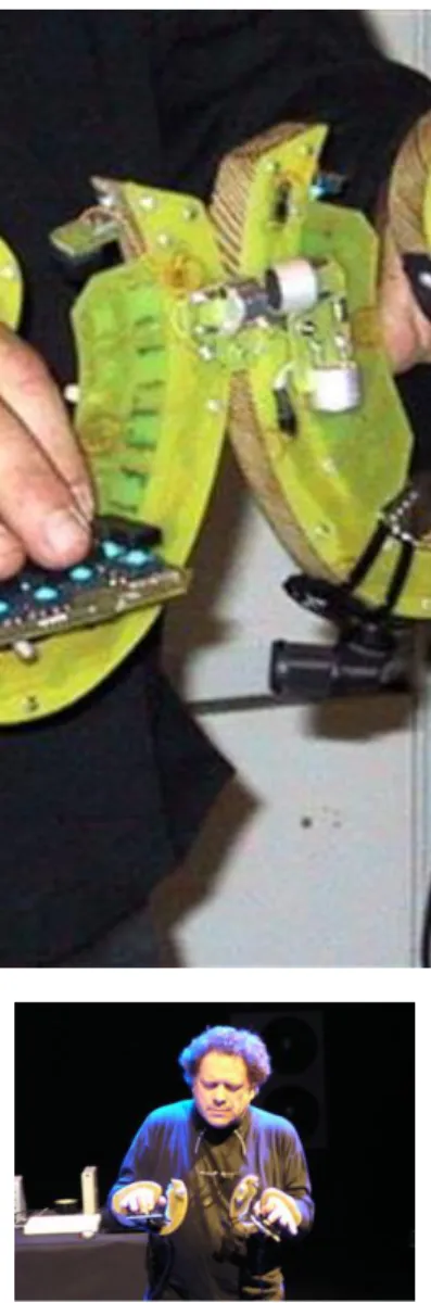
The most obvious and 'ancient' touch controller is the button (allowing the triggering of an event) and the two- state switch, but sliders, dials and other basic controllers, already familiar from common electronic household devices, also belong to this category together with (legacy) computer controllers like joysticks, trackpads or the mouse. Their gestural vocabulary is somewhat limited compared to more advanced controllers, understanding only one (or some of them, two) dimensional motions. Nevertheless, as they have been used as practically the only way to control electronic sound for quite a few decades, some musicians gained a deep experience in mastering these tools. Sophisticated controllers, like The Hands (see Figure 4.7.) combine the ability of playing on keys with built-in motion capturing.
Figure 4.7. The Hands, developed by Michel Waisvisz. An alternate MIDI controller
from as early as 1984.
25
Currently perhaps the most widely used touch controllers are the touch-sensitive 2D screens of tablets, smartphones etc. As these come with highly programmable visual interfaces (and because they are more and more widespread), their usage within the community has constantly been increasing during recent times. Some solutions, like the Reactable (see Figure 4.8.), build on a combination of touch sensing and image recognition - although its control capabilities are very limited.
Figure 4.8. Reactable, developed at the Pompeu Fabra University. The interface
recognises specially designed objects that can be placed on the table and executes the
'patches' designed this way.
27
Expanded-range controllers include tools with limited motion sensing capabilities, like the Radio Baton by Max Matthews (see Figure 4.9.), consisting of two batons and a detector plate, implementing 3D tracking of the location of the baton heads - provided that those are located within a reasonable distance from the detector plate.
Other examples include commercial sensors like the Wii Remote or the gyroscope built into many smartphones.
The Leap Motion, a recent development of 2013, tracks the motion of all 10 fingers individually, allowing the capture of quite sophisticated 3D hand gestures.
Figure 4.9. The Radio Baton (left) and its designer, Max Matthews (right).
Immersive controllers also vary a great amount. They include ambient sensors (like a thermometer) as well as biometrical sensors (like EEG). However, most commonly they are associated with body suits, data gloves, or full-range location sensing (like video-based motion tracking, as implemented by Kinect, depicted in Figure 4.10.).
Figure 4.10. Kinect, by Microsoft.
29