LIMIT CYCLES IN REACTION JET ATTITUDE CONTROL SYSTEMS SUBJECT TO EXTERNAL TORQUES
1 2 λ
P. R. Dahl, G. T. Aldrich, and L. K. Herman Aerospace Corporation, El Segundo, Calif.
ABSTRACT
A great deal of literature has been written on the limit cycle operation of reaction jet attitude control systems and about the nature of external torques such as gravitational, aerodynamic, magnetic, etc, experienced by orbiting satellites.
This paper considers the effects of external torques on the limit cycle operation of a reaction jet attitude control system. Expressions are developed for the impulse require- ments of the limit cycle operation of a system under the action of external torques. Among the results obtained is the interesting fact that destabilizing torques can be used to reduce impulse required below that of a torque free system.
DESCRIPTION
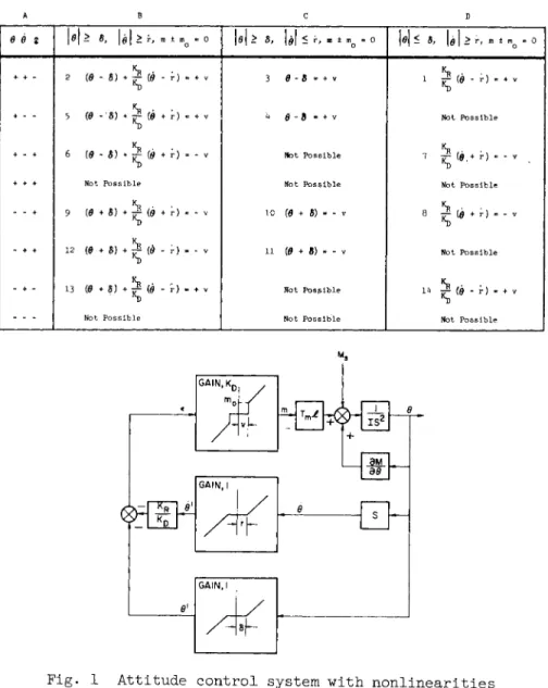
The single-axis attitude control system described by the diagram in Fig. 1 is now considered. The position and rate measurements are considered to have independent and symmetric threshold values δ and r, respectively. A threshold error signal of magnitude ν is necessary to obtain an output from the torque generating device.
The authors consider in particular that the thrust which generates control torque is pulse modulated and the modulation factor is
m = fAt
It is possible to modulate the thrust with pulse frequency f or pulse width At, or both. Fig. 2 depicts the meaning of
Presented at ARS Guidance, Control, and Navigation Conference, Stanford, Calif., Aug. 7 - 9 , I 9 6 1 .
Member of the Technical Staff.
2Member of the Technical Staff.
3Msmber of the Technical Staff.
599
these quantities along with Tm the thrust pulse magnitude.
The time average thrust will obviously saturate for m = 1 but this condition will not be a point of concern in this paper.
SWITCH LINES
The following relations can be written from Fig.
inspection
ο, | β | < δ
θ· = { θ - δ, θ > δ θ + δ, θ < - δ
0, loi < r θ' = J θ - r, θ >r
θ + r, θ < - r 0, |e| < ν
( e - ν) + mo, e > ν
[ KJJ (e + ν) - mo, e <- ν
-e = θ' + ττθ'
1 by _la
"lb 'le
" 2 a
'2b
\2c
' 3 a
'3b
'3c
The equations of the lines, referred to as switch lines, in the phase plane that separate the coasting region from regions where corrective torque is applied may be determined by
setting m ± mQ = 0 in Eqs. 3 b and 3 c The equations of the switch lines can best be found by constructing a table of all the combinations of signs of Θ, Q, and € (see Table l). A set of equations for the θ and $ signals at or above thresh- old are obtained from Eqs. lb, lc, 2 b , 2 c , 3 b , 3 c , and k (see column B, Table l). Another set is obtained by letting β drop below threshold or (θ ± r) = 0 in the equations of column Β (see column C). The remaining possible equations are obtained by letting β drop below the threshold or
(θ - δ) = 0 in the equations of column Β (see column D).
Some of the combinations of signs are not possible and are so indicated. This happens because of the inequalities in the mother set of equations. The segments of the lines defined by the equations in columns B, C, and D which enclose the coast region are plotted in the phase plane diagram of Fig. 3·
[«]
601 POWERED TRAJECTORIES
It is seen that the switch lines defined by Fig. 3 and Table 1 separate regions in the phase plane where the trajectories differ in character. Outside the coast region are powered regions where the trajectories are those where corrective torque is applied. The following trajectory descriptions apply to the system under consideration without external torques.
Regions 1 , 7J 8, and Ik contain rectilinear portions of the trajectories where the control system operates without benefit of position feedback. Regions 2, 5, 6, 9, 1 2 , and 13 contain the second order system spiral portions of the trajectories.
Regions 3j k, 1 0 , and 1 1 contain the elliptical portions of the trajectories where the system operates without benefit of rate feedback.
The regions of importance so far as limit cycles are con- cerned are the coast region and the elliptical trajectories regions, for it can be deduced that the steady limit cycle of the system being considered is determined by r and (S + v).
The vehicle will coast at angular velocity ± r until 0 = ± ( δ + ν), at which time corrective torque is applied without benefit of rate feedback, giving rise to an elliptical trajectory symmetrical about the θ axis. The corrective torque is removed when the point on the elliptical trajectory coincides with a point on a switch line. It should be pointed out that the powered portion of the limit cycle trajectories are elliptical only if the threshold modulation factor m0 = 0.
If m0 4 0, the trajectories tend to be parabolic and are perfect parabolas if m = m0 = constant. When pulse modulation
is used, the minimum angular momentum impulse applied to the vehicle by a single thrust pulse should be much less than Ir or
Τ / A t . = I Δ θ « Ir m m m
in order that the foregoing comments apply. If this is not the case, the mean drift velocity will be determined by
Τ / A t .
• _ n m m m θ - 2 I
where η is the integer number of pulses required to reverse angular rate. Since η should be an integer, it will be some value higher than the reversing impulse or
m m m
Ideally η should be the next integer value above the value of the right side of the above expression. An interesting thing to note is that the number of pulses should lie between that required^to insure a change of sign of Q and that required to change Q from r to -r. Thus
Ir . . ο Ir
<n <2 T i n t - M Τ / At . _ _. .
m m m m m m
and, therefore, the mean drift velocity will be less than r.
For η large, the torque control becomes almost continuous (small granularity), η approaches the right side of Eq. 8 and the drift velocity is approximately r. For η = 1 and
^r/^m^^^min n e a rl y equal to but less than unity, the mean drift velocity approaches τ/2. It would appear that by proper design, an attitude control system using pulse modulation might have a built-in safety margin of gas or propellant supply (in the absence of external torque).
Fig. k illustrates a pulse frequency modulation system response trajectory in the phase plane where the mean drift velocity is slightly greater than r/2. The pulse width in this case is constant. Fig. 5 illustrates a pulse modulation system response trajectory when the pulse width and pulse frequency are both modulated. Position and rate thresholds are not shown in this figure.
COAST TRAJECTORIES
In the absence of external torques, the vehicle will coast with constant angular velocity across the coast region from
switch line to switch line and from left to right in the upper half of the phase plane and from right to left in the lower half of the phase plane.
The characteristics of the coast trajectories when the vehicle is subject to external torques can be determined by solving the vehicle's equation of motion. The equation of motion of the coasting vehicle with a stabilizing or desta- bilizing torque and a steady torque acting on it is
where ΘΜ/θο = stabilizing or destabilizing torque coefficient (ft-lb/radian) and Ms = steady torque (ft/lb). The coefficient 3M/3Ö is defined as the moment (stabilizing or destabilizing) per unit angle Θ.
Considering aerodynamic and gravitational moments acting in the pitch plane on a circular orbital vehicle with pitch attitude deviation β from the local horizontal in the direc- tion of motion, the torque coefficient, ΘΜ/θ0, can be expressed as
Θ Μ m τ 2 fr τ \
Ζθ = Μ0 - 3 ωο ^ χ *Σζ}
where is the aerodynamic stability derivative with respect to 0, Iz is the yaw moment of inertia, Ix is the roll moment of inertia and ω 0 is the vehicle orbit frequency. The second term on the right of this relation is the torque per unit angle θ resulting from the gravity gradient as presented and discussed by Frye and Stearns (l).^ As is pointed out by Frye and Stearns, Davis (7) has shown that this term arises from a combination of the effects of torque due to gravity gradient and centrifugal force of orbital motion. More general relations for the gravity torques, from which one can determine the gravitational torque derivative, are available in the literature ( 3 , 4, 8, 1 3 , 14)· The aerodynamic stability derivative may be deduced from the normal force and axial force characteristics of the vehicle resulting from what may be considered Newtonian or free molecular flow as is discussed by Frye and Stearns (l), and DeBra and Stearns (5, 6 ) .
A steady torque with respect to body axes could arise from solar radiation pressure or winds. In this case, the torque would be "steady" only during the time of year when the orbit plane of an earth satellite would be normal to Earth-sun radius vector. The solar pressure torque would be constant for a vehicle in a circular heliocentric orbit where one axis is kept aligned with the velocity vector. It can also arise from gas ventage, leakage, and from steady aerodynamic moments in a vehicle whose axis of symmetry is not nominally aligned with the orbital velocity vector (l, 4, 1 0 , 1 1 , 1 2 ) .
Eq. 9 m ay be written as
0 = λ 0 + M2
[io]
4
Numbers in parenthesis indicate References at end of paper.
603
where
Δ du/de ι
[ 1 1 ] Δ M
μ s I If Eq. 10 is divided by Q
i - m
à dö λ 2 ϊ + ϊ
θ θ
[ 1 2 ]
Eq. 12 integrates directly to
β - λ θ - 2 μ # = constant [ 1 3 ] If the sign of is positive and μ = 0, the external torque is destabilizing and the result is the equation of a family of hyperbolas with center at the origin and asymptotes with slope ± λ.· These hyperbolic trajectories exist only within the coast region of the phase plane. Figs. 6 and 7 show the two types of limit cycles which are possible assuming that higher order effects will preclude steady limit cycles inside the ones shown. In Fig. 6 the coast trajectories resemble the constant ß condition which is obtained with no torque. In Fig. 7 the coast trajectories are such that θ always has a mean value other than zero and never reaches zero (unless the trajectory follows the asymptotes).
If the sign of is negative and μ = 0, the external torque is stabilizing and we have the equation of a family of ellipses which describe the trajectories in the coast region. Fig. 8
illustrates the lowest frequency steady limit cycle possible with stabilizing torque. Elliptical trajectories are possible
inside the one shown but it is assumed that spurious torques and lags in a practical system will eventually open these out to the one shown.
If λ = 0 and μ is positive, the equation of a family of parabolas is obtained. These parabolas open to the right in the phase plane. Fig. 9 illustrates the steady limit cycle ob- tained assuming that higher-order effects will open out the trajectories that are possible inside the one shown. For μ smaller than that of Fig. 9, the coast trajectory flattens un- til the apex of the parabola coincides with the 0= - (δ + v) switch line and further reduction of μ causes corrective torque application on the left side of the phase plane.
Had the steady torque term μ not been neglected, in the destabilizing and stabilizing external torque types of
trajectories mentioned in the foregoing, its effect would have been to shift the hyperbola's and ellipse's centers along the 0= 0 axis. Figs. 10 and 1 1 show this effect and the result-
ing limit cycle trajectory shapes.
COAST TIME
The ratio of the time of corrective torque application to the drift or coasting time in a practically designed system will likely be of the order of 10$ or less. Thus the period
of the limit cycle in most cases will be dependent primarily upon the drift time. This time can be determined for a system with external torques and can be compared with the drift time of a
system without external torques to obtain an estimate of relative propellant consumption since the amount of propellant expended over a time interval of operation of the system will be proportional to the frequency of the limit cycle.
Eq. 10 may be solved subject to the initial conditions that exist at the beginning of the drifting portion of the limit cycle.
θ(ο) à
and
θ (ο) â
Definition is given of L (ö(t)
Taking the Laplace transform of Eq. 10
Λ
[ 1 5 ] (s2 - λ2) Ο . (s2 -λ 2)
605
Finding the inverse Laplace transform of Eq. 15 obtains for λ 2 positive
"2- (t) = cosh \ t + τ-75- sinh X t
θο ο λ ο
[ 1 6 ] + [cosh \t - l| , λ2 > 0
and for λ 2 negative
θ ^ ο
•ψ (t) = cos|\|t + ffîff sinlXIt
ο ο
+ ζ fl - cos lAlt], χ2 < 0
[17]
The coast time interval from the initial conditions to Ö = 0 is obtained by setting θ (t) =0.
ο
Destabilizing External Torque, λ > 0 with β = 0
The coast time between corrective torque application from Eq. l6 for the limit cycle type shown in Fig. 6, where μ = 0, is
t = -7- tanh
D1 λ 1
(έ) M
where
κ = HÜTT [ > ] Ι λ Ι ο0
Using the identity
4 - ν , "1 1 , /l + x\
tanh χ = — Ζ η
2 V1 - χ7
Eq. 18 can be expressed as
\ - * ' » ( Η τ ) M
which corresponds to the condition Κ > 1 .
The coast time between corrective torque application for the limit cycle shown in Fig. 7 is determined by differentiating Eq. l6 and setting
obtaining
M H S ) M
which corresponds to the condition 0 < Κ < 1 .
Comparing Eqs. 20 and 21 it can be seen that in general 1 . . . IK + 1
λ
Stabilizing External Torque, λ2 < 0 With μ = 0
The coast time between the switch lines for λ 2 < 0 and β = 0 is obtained from Eq. 1 7
t = T ^ T_2_ tan"1
(^j
[ 2 3 ] Steady External Torque, μ Φ 0 With \2 = 0The coast time for the type of trajectory shown in Fig. 9 can be found by differentiating Eq. 1 7 and setting λ = 0 and 0= 0 . This results in the drift time between corrective torque applications
2 0
[ 2 4 ]
6 0 7
t = -
When M is small enough that corrective torque is applied on both sides of the phase plane diagram, Eq. 1 7 is again dif- ferentiated, setting λ = 0 and setting
è = χ Θ20 - V ö0 [ 2 5 ]
to find the drift time. Equation 25 is obtained from Eq. 13 with β = -ßQ where the constant is evaluated using the initial
conditions 0=θο and β = -ßQ. The result is obtained
for the coast time between corrective torque applications.
The value of μ for which the apex of the parabolas coincides with β = - β0 is obtained from Eq. 25 with β = 0. It is what may be termed the critical value of the steady torque
parameter
c RELATIVE PROPELLANT CONSUMPTION
If it is assumed that corrective torque application time is negligible compared to coast time, the propellant consumption will be proportional to corrective torque application fre- quency or inversely proportional to coast time for a given operating time. The relative propellant consumption ψ is defined as (propellant consumption with external torque ) -7 (propellant consumption without external torque).
Destabilizing External Torque
For the case of destabilizing external torque tT
, D 4 ^ 2 [ 2 8 ]
From Eq. 2 1 , using L'Hospital's rule
•à
λ=0θο Δ +
• — "C
σο
[ 2 9 ]
which could have been deduced directly.
Using Eqs. 22 and 29 in Eq. 28 A. 2 „ K + 1 -1
il
I '
κ-
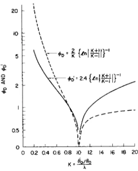
0 [30]It is of interest to see how propellant consumption varies with the destabilizing torque coefficient. Accordingly <f> is plotted vs. l/κ2 in Fig. 1 2 . This figure shows a theoretical relative propellant consumption of zero for Κ = 1 . Prac- tically, less impulse then for the case of a system without torque might be expected if
or
0 < ^ < 1 Λ 4 Κ
0.83 < Κ < co
However, this presumes that the point ($0, ßQ) at which corrective torque is applied, is the same for both conditions (i.e., with torque and with no torque). This behavior is seen in the dashed curve of Fig. 13·
The case is examined where there is a given value of torque and hence λ. It should be possible to vary Κ by virtue of the possibility of adjusting βο/θο- The question may reasonably be asked: What effect does the choice of switching point
(β0, β0) have on propellant consumption? To answer this it may be noticed from Fig. 1 2 that Κ = 0.83 gives the same propellant consumption as the case of zero torque (it may be
considered unity consumption). The ratio is formed
0 n -
Δ tD Wö 0 = °· 8 3 λ
Κ + 1κ
y . èje0= κ λ i ^ n λ
Κ = 0.83 Κ + 1 [ 3 2 ]
609
or
This relation is plotted as curve 1 of Fig. 13 and is
propellant consumption when switched at
9
Q/9
0 = Κ λpropellant consumption when switched at
è
Q/0
o = 0.83 λpropellant consumption when switched at θ0/θ0 = Κ λ r τ propellant consumption when switched at
θ
Q/0
o with\
= 0From the solid curve of Fig. 1 3 , one sees that for a given value of torque
0.83 = < Κ < 1 . 2
[35J
in order that consumption be less than that obtained with zero torque. It is apparent from Eq. 28 that
η
w =η ( I ) M
Something might be gained from this observation; i.e., if the torque coefficient is predictable within a ± per cent
expected error, it would be better to set Κ > 1 because the penalty for error is not so great in this direction as for
Κ < 1 .
In regard to the means for adjusting θ0/θ0> one observes from Fig. 3 that θQ = r and θ0 = δ + ν and, therefore
^o = r
β δ + ν
[»]
As a result, the switching point is easily adjusted if these quantities are at ones disposal in a practical system.
Stabilizing External Torque
The relative propellant consumption for the case where is negative and μ = 0 is obtained using Eq. 23
Equation 3 8 is plotted in Fig. 1 2 which shows that the relative propellant consumption increases monotonically and the con-
sumption with a negative stabilizing external torque coeffi- cient will always be greater than the consumption without torque.
Steady Torque
The relative propellant consumption for the case where χ2 = 0 and μ0 is obtained using Eq. 2k
To obtain the relative propellant consumption for λ = 0 and μ positive and less than μ0, it is assumed that for the corrective torque on the left side of the phase plane, one consumes only
as much fuel in reversing Q as on the right side. The ratio
will then be the relative fuel consumption of this cycle due to the unsymmetric limit cycle. Then the product of this quantity and the ratio of the coast time
6 1 1
1 -
should give a reasonable approximation to the relative fuel consumption. Thus
Eqs. 39 and ^0 are plotted in Fig. Ik, where it is shown that the fuel consumption of the system can be as small as l/h the fuel consumption without external torques.
TOTAL PROPELLANT CONSUMPTION WITHOUT EXTERNAL TORQUE The following assumptions are made:
1) Steady limit cycle only contributes to propellant consumption.
2 ) No external torques.
3) Corrective torque application time negligible compared to coast time.
h) Reaction jets only are used.
One then has the set of equations for a single axis , ο < μ < μ
-2,
t ο
= Nt ο
ψ = τ At Αθ = 2 0
Ο
W
Τ I sp Simple substitutions yield
W
sp ο
Ν
HIGHER-ORDER EFFECTS
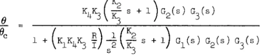
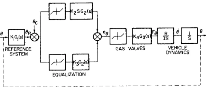
In practical systems the dynamics of the hardware used in the control system lead to higher than second-order system response. Fig. 15 represents a typical single-axis system with the transfer function
s + l)o2(s) G3( S )
1 + (iC^Kg f ) - | ( î Ç S + λ) Gl( s ) G2( s ) G3 ( s )
Fig. l6 presents a comparison between a second-order system, i.e., Gi(s) G2(s) G3(s) equals one, and a higher-order system.
The phase plane is the result of an analog computer study of a system without a threshold in the position channel to the valve. The dynamics of the control system hardware cause the time of switching to lag that of an ideal second-order system thereby increasing limit cycle rates and, subsequently, fuel consumption.
DESIGN CONSIDERATIONS Minimum Pulse Width
The number of pulses to reverse the direction of motion when corrective torque is applied needs to be one or more. Some advantage accrues from a single-thrust pulse as was discussed in the section on Powered Trajectories. If Ν = 1 in Eq. 8 then
Ir < Τ / A t . < 2Ir
m m m
H
6 l J
A pulse width can be found which will cause θ to change its sign and also which will provide some margin of safety such that two corrective pulses will not occur. Choosing a value of torque impulse midway in the range (Eq. 42) one could use
min Τ £ L - i
m
The minimum or threshold pulse width should be at least this small.
Maximum and Minimum Pulse Frequency
If pulse frequency modulation alone is used it is noted that
max At . L J
mm
when m = 1 (or continuous thrust). The minimum pulse fre- quency should be such that l/fmino r ^he time between pulses at threshold conditions is long compared with the instrument
(and possible shaping network) response times. This is desirable to prevent application of more corrective thrust impulses than is necessary because of slow information pro- cessing by control system components. If both of the desired conditions (i.e., fm ax a n (^ ^min) cannot be met because of frequency range limitations of pulse frequency generating devices, it may be desirable to use a combined pulse frequency and pulse width modulation method in order to extend the modulation factor range of the pulse producing equipment.
Adjustments for External Torque
The minimum pulse width should likely be reduced when the vehicle has external torque acting on it. This can be deduced from curve 1 of Fig. 1 3 ; i.e., it is not desirable to allow the single torque impulse to govern AO (unless it corresponds to Κ = l). It is probably better from a design point of view to require something of the order of 1 0 pulses to achieve Ad = 2r in order that the adjustment factor r/ δ + ν pre-
dominate in the determination of relative propellant consumption.
Then again, if r is not accurately known or is time varying in some random way, it may be better to choose Atmj_n to cor- respond to the optimum value of Κ = 1 , providing that minimum pulse width can be accurately set and held time invariant better than r.
CONCLUSIONS
1) In the threshold region or in the vicinity of the origin in the phase plane, trajectories are or can he piecewise linear, hyperbolic, parabolic, and elliptic.
2) Minimum pulse size can affect the mean drift rate ad- vantageously or disadvantageously.
3 ) There may be an advantage in modulating both pulse width and pulse frequency in order to reduce the single pulse impulse below Ir/£ so that it is not the controlling factor in the resulting mean drift rate.
k) With destabilizing torque, the vehicle may drift (hyper- bolic trajectories ) from positive to negative attitudes or the limit cycle may be such as to yield only positive or negative values of attitude.
5) Propellant consumption with destabilizing torque is less than propellant consumption without external torque for values of
a h 1 - " 1 ® '
6) Propellant consumption with destabilizing torque is less than propellant consumption without external torque for values of
if θ0/θ0 ^o r ^ke case of no external torque is
7 ) Propellant consumption with stabilizing torque will be greater than propellant consumption without external torque for a steady powered limit cycle with amplitude determined by the threshold magnitudes.
615
8) Propellant consumption with steady torque is less than propellant consumption without external torque for
< 1
9) Higher-order effects or additional lags in a single—axis attitude control system cause propellant consumption to be greater than a simple second-order system.
1 0 ) Total propellant consumption due to limit cycles in the system without torque is proportional to the square of the rate measurement threshold and inversely proportional to the position measurement threshold plus valve threshold.
1 1 ) Minimum pulse width should be made compatible with the rate measurement threshold.
1 2 ) Minimum pulse frequency should be low compared to sensor cutoff frequencies.
1 3 ) Something of the order of 1 0 pulses should be designed for in the time duration of corrective torque^application.
This should enable the dead zone settings of r, δ , and ν to independently determine the character of the limit cycles.
NOMENCLATURE
f = pulse frequency, pulses/sec
G. = transfer function of i"^ component in control loop, dimensionless
I = moment of inertia (e.g., about pitch axis), slug-ft I = moment of inertia about roll axis, slug-ft2
χ
I = moment of inertia about yaw axis, slug-ft
>d = thrust impulse single corrective torque application, lb-sec
^ = total thrust impulse over operating time, Tip, lb-sec Κ = stabilizing or destabilizing torque parameter,
dimensionless
617
= position gain, dimensionless
= rate gain, sec
= gain of i^*1 component in control loop, dimensionless
£ = moment arm, ft
m = modulation factor (m = 1—constant thrust), dimensionless
m = threshold modulation factor, dimensionless ο
M = steady external torque, ft-lb s
3M/3 β = stabilizing or destabilizing external torque coefficient, ft-lb/radian
η = number of pulses required to reverse angular rate, dimensionless
Ν = total number of thrust impulses in time, Trp, dimensionless
r = rate measurement threshold, radians/sec s = Laplace operator, sec"l
t = time, sec
At = thrust pulse width, sec
A t . = minimum thrust pulse width, sec m m
tp = coast time with destabilizing external torque, sec t = coast time without external torque, sec
t = coast time with destabilizing external torque, sec s
t = coast time with steady external torque, sec Τ = thrust pulse magnitude, lb
m
= system operating time, sec
ν = thrust generator threshold, dimensionless
WT = total propellant used in time T^, lb ,δ = position measurement threshold, radians
e = error signal, radians
β = vehicle Euler angle, radians
β 1 = position measurement signal, radians
Λ
β = Laplace transformed position, radians
0 = initial condition in 0 (beginning of coast), radians 0ç = position command signal, radians
β = vehicle angular rate, radians/sec β1 = rate measurement signal, radians/sec
0 = initial condition in β (beginning of coast ), radians/sec
A 0 = angular rate reversal magnitude, radians/sec
ρ λ = stabilizing or destabilizing torque parameter, sec"
μ = steady external torque parameter, radians/sec2
μ = critical value of steady torque parameter, radians/sec2
φ = relative propellant consumption - destabilizing
" torque, dimensionless
φ^ = relative propellant consumption - stabilizing torque, dimensionless
ψ = relative propellant consumption - stabilizing torque, dimensionless
φ = relative propellant consumption - steady torque,
^ dimensionless
ω = orbit frequency, radians/sec
REFERENCES
1 Frye, W.E. and Stearns, E.V.Β., "Stabilization and attitude control of satellite vehicles," ARS J. 2£, 927-931
(1959).
2 Freeman, G.W., "Limit-cycle efficiency of on-off reaction control systems," Proc. IAS National Specialists Meeting on Guidance of Aerospace Vehicles, Boston, Mass., May 2 5 - 2 7 , i 9 6 0 .
3 Roberson, R.E., "Gravitational torque on a satellite vehicle," J. Franklin Instit. 265, 13 ( 1 9 5 8 ) .
k Roberson, R.E., "Attitude control of a satellite vehicle - an outline of the problems," in Proc. VIII Congress IAF, Barcelona, 1 9 5 7 ; Ρ· 3 1 7 ·
5 DeBra, D.B. and Stearns, E.V., "Attitude control," Elect.
Eng. vol. 7 7 ; I 9 5 8 .
6 DeBra, D.B., "The effect of aerodynamic forces on satellite attitude," in Proc Am. Astronaut S o c , Western Regional Meeting, Aug. 1 9 5 8 .
7 Davis, W.R., "Determination of a unique attitude for an earth satellite, " in Proc. Am. Astronaut. S o c , Fourth Annual Meeting, Jan. 1 9 5 8 .
8 Nesbit, R.A., "Gravity Gradient Torques," Aerospace Corp.
Document A- 6 1 - I 7 3 2 . 2 - l 8 , 1 9 May 1 9 6 1 .
9 Frick, R.H. and Garber, T.B., "General Equations of Motion of a Satellite in a Gravitational Gradient Field," Rand
Document RM-2527.
10 Sohn, R.L., "Attitude stabilization by means of solar radiation pressure," ARS J., 2£, no 5; 371-373 ( 1 9 5 9 ) ·
1 1 Hibbard, R.R., "Attitude stabilization using focused radiation pressure," ARS J., 3 1 , no 6, 8kk-Qk5 ( 1 9 6 1 ) .
1 2 Newton, R.R., "Stabilizing a spherical satellite by radiation pressure," ARS J. 30, no 1 2 , I I 7 5- I I 7 7 ( i 9 6 0 ) .
13 Hultquist, P.F., "Gravitational torque impulse on a stabilized satellite," ARS J., 3 1 , no 1 1 , I506-I5O9 ( 1 9 6 1 ) .
lk Roberson, R.E., "Gravity gradient determination of the vertical," ARS J. 3 1 , no 1 1 , 1 5 0 9 - 1 5 1 5 ( I 9 6 l ) ·
619
θ ζ M > s, |â|>r, |ö| > 5, 101 < r, m ± m - 0 \θ\< δ, \è\>r, m
2 (0 - 6) + f (0 - r)
5 (0 - δ ) + ^ (0 + r)
6 (0 - δ) + / (0 + r)
N o t P o s s i b l e
9 (0 • β) + / (0 + r) :
12 (β + δ) + £ (d - r) « -
KR · · 13 (0 + δ) + -f (0 - Γ ) - +
N o t P o s s i b l e
3 β - δ = + ν
h $ - 8 - + ν
N o t P o s s i b l e
N o t P o s s i b l e
I C (0 + β) « - ν
11 (0 + δ) « - ν
N o t P o s g i b l e
N o t P o s s i b l e
1 IT (0 - r) « + ν
Not P o s s i b l e
KR - -
7 FM0.+ r ) '
Not P o s s i b l e
KR · -
N o t P o s s i b l e
1^ ^ (0 - r) - + ι Not P o s s i b l e
Fig. 1 Attitude control system with nonlinearities
A t
Fig. 2 Reaction jet thrust wave form
62h
Fig. Ik Steady torque relative propellant consumption
K,G,(s) REFERENCE
S Y S T E M
K2S G2( s ) J - j
m _R_
I S GAS VALVES
E Q U A L I Z A T I O N
V E H I C L E I DYNAMICS I
15 Attitude control system with nonlinearities and higher order effects
SWITCH LINES HIGHER ORDER SYSTEM LIMIT CYCLE
Fig. l6 Higher order system effects
627