(2010) pp. 51–75
http://ami.ektf.hu
Evaluating a probabilistic model checker for modeling and analyzing retrial queueing
systems ∗
Tamás Bérczes
a, Gábor Guta
b, Gábor Kusper
cWolfgang Schreiner
b, János Sztrik
aaFaculty of Informatics, University of Debrecen, Hungary
bResearch Institute for Symbolic Computation (RISC), Johannes Kepler University, Linz, Austria
cEszterházy Károly College, Eger, Hungary
Submitted 6 April 2009; Accepted 27 May 2010
Dedicated to professor Béla Pelle on his 80th birthday
Abstract
We describe the results of analyzing the performance model of a finite- source retrial queueing system with the probabilistic model checker PRISM.
The system has been previously investigated with the help of the performance modeling environment MOSEL; we are able to accurately reproduce the re- sults reported in literature. The present paper compares PRISM and MOSEL with respect to their modeling languages and ways of specifying performance queries and benchmark the executions of the tools.
1. Introduction
The performance analysis of computing and communicating systems has always been an important subject of computer science. The goal of this analysis is to make predictions about the quantitative behavior of a system under varying con- ditions, e.g., the expected response time of a server under varying numbers of
∗The work is supported by the TÁMOP 4.2.1./B-09/1/KONV-2010-0007 project. The project is implemented through the New Hungary Development Plan, co-financed by the European Social Fund and the European Regional Development Fund.
51
service requests, the average utilization of a communication channel under varying numbers of communication requests, and so on.
To perform such an analysis, however, first an adequate mathematical model of the system has to be developed which comprises the interesting aspects of the sys- tem but abstracts away from details that are irrelevant to the questions addressed.
Originally, these models were developed purely by manual efforts, typically in for- mal frameworks based on queuing theory, stochastic Petri networks, and the like, which can be ultimately translated into continuous time Markov chains (CTMCs) as the fundamental mathematical basis [18]. Since the manual creation of com- plex models is tedious and error-prone, specification languages and corresponding tools were developed that automated the model creation from high-level system descriptions. Since the generated models cannot typically be solved analytically, simulation-based techniques were applied in order to predict their quantitative behavior from a large number of sampled system runs. Latter on, however, the underlying systems of equations were solved (for fixed parameter values) by iter- ative numerical calculations, thus deriving (mathematically exact but numerically approximated) solutions for the long-term (steady state) behavior of the system.
One tool of this kind is MOSEL (Modeling, Specification, and Evaluation Lan- guage) [14, 3] with its latest incarnation MOSEL-2 [15]. The software has a high- level specification language for modeling interconnected queue networks where tran- sitions execute at certain rates to move entities across queues. The environment supports various back ends for simulating the model system or for computing nu- merical solutions of the derived system of steady-state equations. In particular, it may construct a stochastic Petri net model as input to the SPNP solver [10].
While above developments emerged in the performance modeling and evalu- ation community, also the formal methods community has produced theoretical frameworks and supporting tools that are, while coming from a different direction, nevertheless applicable to performance analysis problems. Originally, the only goal of formal methods was to determine qualitative properties of systems, i.e., prop- erties that can be expressed by formal specifications (typically in the language of temporal logic).
In the last couple of years, however, the formal methods community also got more and more interested in systems that exhibit stochastic behavior, i.e., systems whose transitions are executed according to specific rates (respectively probabili- ties); this gives rise to continuous time (respectively discrete time) Markov chains like those used by the performance modeling community and to questions about quantitative rather than qualitative system properties. To pursue this new direc- tion of quantitative verification [12], model checking techniques were correspond- ingly extended tostochastic/probabilistic model checking [13].
A prominent tool in this category is the probabilistic model checker PRISM [16, 9] which provides a high-level modeling language for describing systems that ex- hibit probabilistic behavior, with models based on continuous-time Markov chains (CTMCs) as well as discrete-time Markov chains (DTMCs) and Markov decision procedures (MDPs). For specifying system properties, PRISM uses the probabilis-
tic logics CSL (continuous stochastic logic) for CTMCs and PCTL (probabilistic computation tree logic) for DTMCs and MDPs, both logics being extensions of CTL (computation tree logic), a temporal logic that is used in various classical model checkers for specifying properties [7]. While some probabilistic model check- ers are faster, PRISM provides a comparatively comfortable modeling language;
for a more detailed comparison, see [11].
The fact that the previously disjoint areas of performance evaluation and formal methods have become overlapping is recognized by both communities. While origi- nally only individual authors hailed this convergence [8], today various conferences and workshops are intended to make both communities more aware of each others’
achievements [5, 21]. One attempt towards this goal is to compare techniques and tools from both communities by concrete application studies. The present paper is aimed at exactly this direction.
The starting point of our investigation is the paper [19] which discusses various performance modeling tools; in particular, it presents the application of MOSEL to the modeling and analysis of a retrial queuing system previously described in [1]
and latter refined in [17]. The goal of the present paper is to construct PRISM models analogous to the MOSEL models presented in [19] for computing the per- formance measures presented in the above paper, to compare the results derived by PRISM with those from MOSEL, to evaluate the usability and expressiveness of both frameworks with respect to these tasks, to benchmark the tools with respect to their efficiency (time and memory consumption), and finally to draw some over- all conclusions about the suitability of PRISM to performance modeling compared with classical tools in this area.
The rest of the paper (which is based on the more detailed technical report [4]) is structured as follows: Section 2 describes the application to be modeled and the questions to be asked about the model; Section 3 summarizes the previously presented MOSEL solution; Section 4 presents the newly developed PRISM solu- tion; Section 5 gives the experimental results computed by PRISM in comparison to those computed by MOSEL and also gives benchmarks of both tools; Section 6 concludes and gives an outlook on further work.
2. Problem description
2.1. Problem overview
In this section we give a brief overview on the model of the retrial queueing system presented in [19]. The variable names used latter in the model are indicated in italics in the textual description. The dynamic behavior of the model is illustrated by UML state machine diagrams [20].
The system contains a single server and NT terminals. Their behavior is as follows:
• Intuitively, terminals send requests to the server for processing. If the server is busy, the terminals retry to send the request latter. More precisely, the
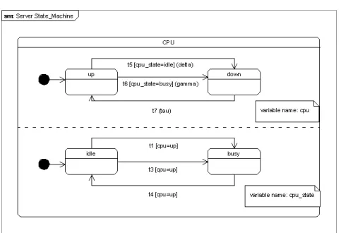
Figure 1: State machine representation of the server
terminals can be in three different states (which are named in parentheses):
1. ready to generate a primary call (busy), 2. sending repeated calls (retrying) and 3. under service by the server (waiting).
• The server according to its CPU state (cpu) can be operational (cpu=cpu_up) or non-operational (cpu=cpu_down): if it is operational we distinguish be- tween two further states (cpu_state): idle (cpu_state=cpu_idle) and busy (cpu_state=cpu_busy).
• In the initial state of the system, the server is operational (cpu=cpu_up) waiting for requests (cpu_state=cpu_idle) and all terminals are ready to generate a primary call.
2.2. Finite state model
The behavior of the system can be described by the state transitions of the terminals and the server, which occur at different rates.
We extend the standard UML [20] state machine diagram notation and seman- tics to present our model in an easy-to-read way. According to the standard, the diagram contains states and transitions; the transitions in different swim-lanes can occur independently. Our extensions are the following:
• Every comment of a swim-lane contains a variable name which is changed by the transition of that lane.
• Each transition is associated with a triple of a label, a guard (in square brackets) and a rate(in parentheses); if there is no rate indicated, then the rate equals 1.
• A parallel composition semantics: the set of the states of the composed system is the Cartesian product of the state sets of the two swim-lanes or state machines. The composed state machines can make a transition whenever one of the original state machines can make one, except if multiple transitions in different original state machines have the same label: it that case, they must be taken simultaneously.
In Figure 1 we show the state transitions of the server:
t1 (The server starts to serve a primary call) If the server is in operational state and idle, it can receive a primary call and become busy.
t2 (The server rejects to serve a primary call) If the server is operational and busy, it can reject a primary call.
t3 (The server starts to serve a retried call) If the server is in operational state and idle, it can start to serve a repeated call.
t4 (The server finishes a call) If the server is operational and busy, it can finish the processing of the call.
t5 (An idle server becomes inoperable) If the server is in operational state and idle, it can become inoperable with rateδ.
t6 (A busy server becomes inoperable) If the server is in operational state and busy, it can become inoperable with rateγ.
t7 (A server gets repaired) If the server is inoperable, it can become operable again with rateτ.
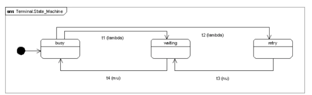
The state transitions of the terminal are described in Figure 2:
t1 (The server starts to serve a primary call) The call of a terminal which issues a primary call is accepted and it becomes a waiting terminal with probabilityλ.
t2 (The server rejects a primary call) The call of a terminal which issues a primary call is rejected and it becomes a retrying terminal with probabilityλ.
t3 (The server starts to serve a retried call) The call of a terminal which re- tries a call is accepted and it becomes a waiting terminal with probabilityν.
t4 (The server finishes a call) The call of a terminal is finished and it becomes ready to generate a new primary call again with rateµ.
Figure 2: State machine representation of the terminals
The system can be represented alternatively by merging the server and the terminals into a single system as modelled in the original MOSEL model [19]: the guard conditions of all transitions with the same label are logically conjoined and their probabilities are multiplied.
2.3. Mathematical model
In this section we describe the mathematical formulation of the queries. The state of the system at time t can be described by the process X(t)=(cpu(t), cpu_state(t), retrying_terminals(t)), where cpu(t)=0 (cpu_up) if the server is operable, cpu(t)=1 (cpu_ down) if the server is not operable, cpu_state(t)=0 (cpu_idle) if the server is idle andcpu_state(t)=1 (cpu_busy) if the server is busy and retrying_terminals(t) describe the number of repeated calls at time t. The number of waiting terminals and busy terminals are not expressed explicitly in the mathematical model. Their values can be calculated according to the following equations:
• waiting_terminals=0 ifcpu_state=cpu_idle,
• waiting_terminals=1 ifcpu_state=cpu_busy,
• busy_terminals=NT-(waiting_terminals+retrying_terminals),
Because of the exponentiality of the involved random variables and the finite number of sources, this process is a Markov chain with a finite state space. Since the state space of the process X(t), t >0 is finite, the process is ergodic for all reasonable values of the rates involved in the model construction. From now on, we assume that the system is in the steady-state.
We define the stationary probabilities by:
P(q, r, j) = lim
t→∞P(cpu(t), cpu_state(t), retrying_terminals(t)), q= 0,1, r= 0,1, j= 0,· · · , N T−1,
The main steady-state system performance measures can be derived as follows:
• Utilization of the servers
cpuutil=
N TX−1
j=0
P(0,1, j)
• Availability of the servers
goodcpu= X1
r=0 N TX−1
j=0
P(0, r, j)
• Utilization of the repairman
repairutil= X1
r=0 N TX−1
j=0
P(1, r, j) = 1−goodcpu
• Mean rate of generation of primary calls
busyterm=E[N T −cpu_state(t)−retrying_terminals(t);cpu(t) = 0]
= X1
r=0 N TX−1
j=0
(N T −r−j)P(0, r, j)
• Utilization of the sources
termutil= busyterm N T
• Mean rate of generation of repeated calls
retravg=E[retrying_terminals(t);cpu(t) = 0] = X1
r=0 N TX−1
j=0
jP(0, r, j)
• Mean number of calls staying in the server
waitall=E[cpu_state(t)] = X1
q=0 N T−1X
j=0
P(q,1, j)
• Mean number of calls staying in the orbit
retrall=E[retrying_terminals(t)] = X1
q=0
X1
r=0 N TX−1
j=0
jP(q, r, j)
• Overall utilization
overallutil=cpuutil+repairutil+N T ∗termutil
• Mean number of calls staying in the orbit or in the server meanorbit=waitall+retrall
• Mean response times
E[T] =E[retrying_terminals(t)] +E[cpu_state(t)]
λ∗busyterm
The last equation is essentially a consequence ofLittle’s Theorem, a classical result in queuing theory [6], which describes for a queuing system in equilibrium by the equationT =L/λthe relationship between the long-term average waiting time T of a request, the long-term average number of requests L pending in the system, and the long-term average request arrival rateλ. Furthermore, according toJackson’s Theorem, a network ofN queues with arrival ratesλmay (under rather loose assumptions) be considered as a single queue with arrival rateλ¯=λN. This relationship will become crucial in the use of MOSEL and PRISM described in the following sections because it allows us to reduce questions about average timing properties of a system to questions about quantities which can be deduced from the (long-term) observation of states.
2.4. Questions about the system
Our goal is to study various quantitative properties of the presented models to get a deeper understanding of the modelled systems. The following properties are analyzed:
cpuutil The ratio of the time the server spends serving calls compared to the total execution time (06cpuutil61).
goodcpu The ratio of the time when the server is operable compared to the total execution time (06goodcpu61).
repairutil The ratio of the time when the server is inoperable compared to the total execution time (06repairutil61).
busyterm The average number of served terminals while the system is operable (06busyterm6NT).
termutil The ratio of served terminals while the system is operable to the total number of terminals (06termutil61).
retravg The average number of retrying terminals while the system is operable (06retravg6NT−1).
waitall The average number of waiting terminals during the total system execution time (06waitall61).
retrall The average number of retrying terminals during the total system execu- tion time (06retrall6NT-1).
overallutil The sum of the system average utilization, i.e., the sum of cpuutil, repairutil andNT*termutil (06overallutil6NT+1).
meanorbit The average number of retrying terminals and waiting terminals dur- ing the total system execution time (06retrall6NT).
resptime The mean response time, i.e., the average waiting time till a call of a terminal is successfully accepted.
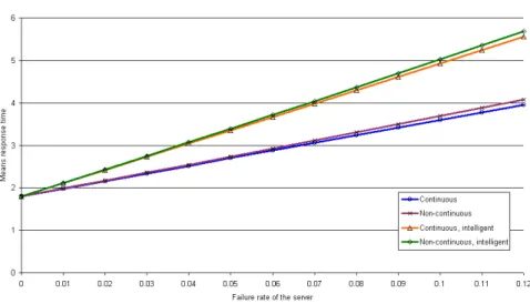
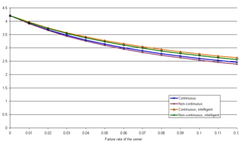
2.5. Different versions of the system
In [19], actually four slightly different systems were described:
continuous The presented model.
non-continuous If the server becomes inoperable, then the call has to be retried (the waiting terminal becomes retrying).
continuous, intelligent It can also reject a call if the server is inoperable (the original model cannot handle a call if the server is inoperable.
non-continuous, intelligent The combination of the non-continuous and intel- ligent model.
The latter three variants are not formally described in the present paper. However, they have been implemented and have been used for the experiments in Section 5.
3. Modeling and analyzing in MOSEL
The MOSEL language (Modeling Specification and Evaluation Language) was de- veloped at the University of Erlangen. The MOSEL system uses a macro-like language to model communication networks and computer systems, like stochastic Petri nets. The MOSEL tool contains some language features, like variables and functions in the style of the C programming language. The MOSEL system calls an external tool after having translated the MOSEL code into the respective tool’s format. For example the Petri net analysis tool SPNP and the state analysis tool MOSES can be used. Because of page limitation the interested reader is referred to [4] where the source codes and technical details of our MOSEL model can be found.
4. Modeling and analyzing in PRISM
In this section we describe how we translate the model described in Section 2 into a PRISM model. Further information about the PRISM system can be found in [16]. In the first subsection we show the source-code of the PRISM model; in the second subsection we formulate questions in the model.
4.1. Translating the model to PRISM
In this subsection and the following ones, we present the full source code of the PRISM model (in verbatim) surrounded by detailed comments. The model de- scription has 4 main parts:
• the type of the model,
• the constant declarations,
• the module declarations and
• the reward specifications.
In our case, all models are represented in Continuous-time Markov chains model, which is indicated by the keywordstochastic.
stochastic
Constants can be used in two manners:
• uninitialized constants denote parameters of the model and,
• initialized constants denote fixed values.
The parameters of the model are the following constants:
const int NT; // number of terminals
const double lambda; // the rate of primary call generation const double mu; // the rate of the call servicing
const double nu; // the rate of repeated call generation
const double delta; // the failure rate in idle state of the server const double gamma; // the failure rate in busy state of the server const double tau; // the repair rate of the server
In our simulation we do not distinguish between the failure rate in idle and busy state, so we equalgammawithdelta.
We define two pairs of constants to represent the state of the server to make the model human-readable:
const int cpu_up = 0; // the server is operable const int cpu_down = 1; // or not
const int cpu_busy = 0; // the server is busy serving a call const int cpu_idle = 1; // or idle waiting for a call
The next fragment are the module definitions. A module definition is started with themodulekeyword and is closed with theendmodulekeyword. All modules contain state variables and state transitions. We have two modulesTERMINALSand SERVERdescribed in the following subsections
4.2. Terminals
The module TERMINALSrepresents the set of the terminals. We keep track of the number of terminals in specific states, because in PRISM it is not possible to have multiple instances of a module. Thus all variables range from 0 to the maximal number of terminals, which is denoted by the range indicator within square brackets in the source code.
module TERMINALS
busyTs : [0..NT] init NT;
retryingTs : [0..NT] init 0;
waitingTs : [0..NT] init 0;
We have the following variables in the model :
• busyTs is the number of terminals, which are capable to generate primary calls (they are busy with local tasks and may generate calls to the server);
• retryingTsis the number of retrying terminals, i.e., terminals which have generated an unsuccessful call and are retrying the same call;
• waitingTs is the number of waiting terminals, i.e., terminals which have issued a successful call to the server and wait for the answer of the call.
In the current model, we have only one server, therefore the number of waiting terminals never be more than 1. Initially all terminals are busy terminals.
The transitions are represented in form[l] g -> r : u. The transition with label l occurs if the guard g evaluates to true; the rate of the transition is r, the values of the state variables are updated according to u. The labels serve as synchronization identifiers for parallel composition. Transitions with the same label in different modules execute together, i.e., all guards of the transition must be true and the total transition rate is the product of the individual transition rates. We also have to notice that the transitions of the terminals have their counterparts on the server side, which make the transition guards unique.
The transition with labelt1describes the scenario of a successful primary call:
[t1] busyTs > 0 & waitingTs < NT -> lambda*busyTs : (busyTs’ = busyTs-1) & (waitingTs’ = waitingTs+1);
The transition occurs if there are some busy terminals and the number of waiting terminals is lower than the number of terminals. The second part of the guard condition is purely technical to explicitly state that the value of waitingTsis not
greater than the maximally allowed value. (According to the model semantics we know that it never becomes greater than one, because the server serves only one call at once.) All busy terminals produce that call with rate λ, so the rate is λ multiplied by the number of busy terminals. After that transition, the number of busy terminals decreases by one and the number of busy terminals increases by one.
The transition with labelt2describes the scenario of an unsuccessful primary call:
[t2] busyTs > 0 & retryingTs < NT -> lambda*busyTs : (busyTs’ = busyTs-1) & (retryingTs’ = retryingTs+1);
The transition occurs if there are some busy terminals and the number of retry- ing terminals is lower than the number of terminals. The second part of the guard condition is also purely technical to explicitly state that the value of waitingTsis not greater than the maximally allowed value. (According the model semantics we know that it never becomes grater than maximal number, because the sum of the terminal variables equals the number of terminals.) All busy terminals produce that call with rate λ, so the rate is λ multiplied by the number of busy termi- nals. After that transition the number of busy terminals decreases by one and the number of busy terminal increases by one.
The transition with label t3 describes the scenario of a successfully repeated call:
[t3] retryingTs > 0 & waitingTs < NT -> nu*retryingTs : (retryingTs’ = retryingTs-1) & (waitingTs’ = waitingTs+1);
The transition occurs if there are some retrying terminals and the number of waiting terminals is smaller than the number of terminals. All retrying terminals produce the calls with rate ν, so the rate is ν multiplied by the number of busy terminals. After that transition, the number of retrying terminals decreases by one and the number of waiting terminals increases by one.
The transition with label t4describes the scenario of an answer for a waiting terminal:
[t4] waitingTs > 0 & busyTs < NT -> 1 :
(waitingTs’ = waitingTs-1) & (busyTs’ = busyTs+1);
The transition occurs if there are some waiting terminals and the number of busy terminals smaller than the number of terminals. Its rate is determined by the call serving rate on the server side (see below). After that transition, the number of retrying terminals decreases by one and the number of waiting terminals increases by one.
endmodule
4.3. Server
The second module represents the server by two binary state variables. The variable cpuexpresses the operability of the server by the values 0 and 1, which are denoted by the constantscpu_upandcpu_down, respectively. The variablecpu_statethe state of the server by values 0 and 1, which are denoted by the constantscpu_busy andcpu_idle, respectively.
module SERVER
cpu : [cpu_up..cpu_down] init cpu_up;
cpu_state : [cpu_busy..cpu_idle] init cpu_idle;
The transition with labelt1 describes the server side scenario of a successful primary call. It occurs, if the server is operable and idle. After the transition, the server becomes busy.
[t1] cpu = cpu_up & cpu_state = cpu_idle -> 1 : (cpu_state’ = cpu_busy);
The transition with labelt2describes the server side scenario of an unsuccessful primary call. It occurs, if the server is operable and busy. After the transition, the state of the server doesn’t change.
[t2] cpu = cpu_up & cpu_state = cpu_busy -> 1 : (cpu’ = cpu) & (cpu_state’ = cpu_state);
The transition with labelt3 describes the server side scenario of a successful primary call. It is the same as the transitiont1, because the server can’t distinguish between a primary and a repeated call.
[t3] cpu = cpu_up & cpu_state = cpu_idle -> 1 : (cpu_state’ = cpu_busy);
The transition with labelt4describes the server side scenario of finishing a call (a successful call served). It occurs with rate µ and the server becomes idle after the transition.
[t4] cpu = cpu_up & cpu_state = cpu_busy & mu > 0 -> mu : (cpu_state’ = cpu_idle);
The transition with labelt5describes the scenario when an idle server becomes inoperable. It occurs, if the server is operable and idle with rate γ. If a server becomes inoperable, it keeps its state. After it gets repaired, it continues the processing, if it was busy at the time of the failure.
[t5] cpu_state = cpu_idle & cpu = cpu_up & delta > 0 -> delta : (cpu’ = cpu_down);
The transition with labelt6describes the scenario when a busy server becomes inoperable. It occurs, if the server is operable and busy with rateδ.
[t6] cpu_state = cpu_busy & cpu = cpu_up & gamma > 0 -> gamma : (cpu’ = cpu_down);
The transition with labelt7describes the scenario when a server gets repaired.
It occurs, if the server is inoperable with rateτ.
[t7] cpu = cpu_down & tau > 0 -> tau : (cpu’ = cpu_up);
endmodule
4.4. Rewards
The last section of a model description is the declaration of rewards. Rewards are numerical values assigned to states or to transitions. Arbitrary many reward structures can be defined over the model and they can referenced by a label. We use rewards to define the various question defined in Section 2.4.
The first reward is the server utilization (cpuutil). It assigns a value 1 to all states where the server is operable and busy.
rewards "cpuutil"
cpu = cpu_up & cpu_state = cpu_busy : 1;
endrewards
The rewardgoodcpu assigns 1 to all states where the server is operable.
rewards "goodcpu" cpu = cpu_up : 1; endrewards
The rewardrepairutil assigns 1 to all states where the server is inoperable.
rewards "repairutil" cpu = cpu_down : 1; endrewards
The rewardbusyterm assigns the number of busy terminals to all states where the server is operable.
rewards "busyterm" cpu = cpu_up : busyTs; endrewards
The rewardtermutilassigns the ratio of the busy terminals over the total num- ber of terminals to all states where the server is operable.
rewards "termutil" cpu = cpu_up : busyTs/NT; endrewards
The rewardretravg assigns the number of retrying terminals to all states where the server is operable.
rewards "retravg" cpu = cpu_up : retryingTs; endrewards
The rewardwaitall assigns the number of waiting terminals to states with such terminals.
rewards "waitall" waitingTs > 0 : waitingTs; endrewards
The rewardwaitall assigns the number of retrying terminals to states with such terminals.
rewards "retrall" retryingTs > 0 : retryingTs; endrewards
The rewardmeanorbit assigns the number of retrying and waiting terminals to states with such terminals.
rewards "meanorbit"
retryingTs > 0 : retryingTs;
waitingTs > 0 : waitingTs;
endrewards
The rewardpending computes the number of pending calls (calls by terminals that are waiting or retrying); the relevance of this reward for computing the mean response time response will be explained in the next subsection.
rewards "pending"
retryingTs > 0 : retryingTs;
waitingTs > 0 : waitingTs;
endrewards
The reward overallutil assigns to the all states the total number of all busy elements, i.e., the server, if it is busy or is under repair (a repair unit is busy with its repair), and all busy terminals.
rewards "overallutil"
cpu = cpu_up & cpu_state = cpu_busy : 1;
cpu = cpu_down : 1 ; cpu = cpu_up : busyTs;
endrewards
4.5. Questions about the System in PRISM
As we mentioned in the introduction, in PRISM the queries about the CTMC models can be formulated in CSL (Continuous Stochastic Logic). CSL is a branch- ing-time logic similar to CTL or PCTL [2]. It is capable to express queries about both transient and steady-state properties. Transient properties refers to the values of the rewards at certain times and the steady-state properties refer to long-run rewards.
The PRISM system support not only evaluating predicates about the rewards, but also queries about the rewards. In our experiments we used only the following one CSL construction: R{"l"}=? [ S ]. This query ask for the expected long-run reward of the structure labelled with l. Most questions about the model described in Section 2.4 can be formulated as CSL expressions.
R{"cpuutil"}=? [ S ] R{"goodcpu"}=? [ S ] R{"repairuti"}=? [ S ] R{"busyterm"}=? [ S ] R{"termutil"}=? [ S ] R{"retravg"}=? [ S ] R{"waitall"}=? [ S ] R{"retrall"}=? [ S ] R{"overallutil"}=? [ S ] R{"meanorbit"}=? [ S ]
The response time (resptime) cannot be directly calculated from a CSL query, because CSL does not allow us to ask questions about execution times (rather than say probabilities or long-term average rewards). We rather resort to queuing theory and apply the definition of E[T]stated in Section 2 which can be expressed as
resptime=pending/(lambda*busyterm)
Since this calculation is not directly expressible as a CSL query, we apply a post- processor to computeresptimefrom the values forpendingandbusytermgener- ated by PRISM from above CSL queries. Similar to MOSEL, we can thus reduce questions about timing properties of a system to the computation of quantities that can be derived from system states and are thus amenable to CSL queries in PRISM.
5. Experimental results
In this section, we show the result of the experiments carried through with PRISM.
The parameters used for the experiments are listed in Figure 4; they are the same as published in [19]. The results of the experiments with PRISM are presented in diagrams Figure 5, 6, 7, 8, 9, 10, whereas the raw results can be seen in Tables in [4].
The experiments was performed in two main steps: the execution of the ex- periments through the GUI of PRISM and the post-processing of the results. We selected the appropriate CSL query according the Figure 3 and set up the parame- ters according the Figure 4; after the execution of PRISM the results were exported to CSV files for further processing. The post processing happened with a help of Python scripts.
5.1. Analysis results
The diagrams compared with the ones presented in [19] clearly show that the two models (MOSEL and PRISM) produce identical results for the same parameters.
Comparing the raw results of the experiments, it shows that they are differ only after the 5th decimal digit. The quality of the results produced with PRISM is this the same as the ones produced in MOSEL.
Nr. of the experiment used reward(s)
1 pending and termutil
2 overallutil
3 meanorbit
4 pending and termutil
5 overallutil
6 meanorbit
Figure 3: Rewards calculated in the experiments
Exp. Nr. NT λ µ ν γ/δ τ X axis
1 6 0.8 4 0.5 X axis 0.1 0. 0.01. ..., 0.12 2 6 0.1 0.5 0.5 X axis 0.1 0. 0.01. ..., 0.12 3 6 0.1 0.5 0.05 X axis 0.1 0. 0.01. ..., 0.12 4 6 0.8 4 0.5 0.05 X axis 0.5. 1.0. ..., 4.0 5 6 0.05 0.3 0.2 0.05 X axis 0.5. 1.0. ..., 4.0 6 6 0.1 0.5 0.05 0.05 X axis 0.5. 1.0. ..., 4.0
Figure 4: Parameters of the experiments
Figure 5: Results of the 1st experiment
Figure 6: Results of the 2nd experiment
Figure 7: Results of the 3rd experiment
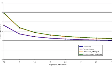
Figure 8: Results of the 4th experiment
Figure 9: Results of the 5th experiment
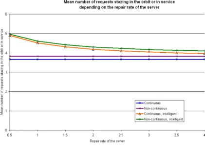
Figure 10: Results of the 6th experiment
5.2. Tool benchmarks
A benchmark was carried through to compare the efficiency of the two tools. The parameters of the machine that was used for the benchmark: P4 2.6GHz with 512KB L2 Cache and 512MB of main memory. Unfortunately MOSEL is not capable to handle models where the number of terminals (NT) is greater than 126, such that the runtime of the benchmarks (which in PRISM especially depend on NT) remain rather small.
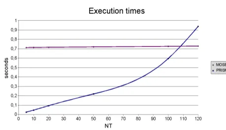
Both of the tools were tested with the described model using the following parameters: λ=0.05,µ=0.3,ν =0.2,γ=δ=0.05,τ =0.1. The comparison of the two tools can be seen in Figure 11 and Figure 12. In Figure 13, we can see a more detailed description of the PRISM benchmark (the times of the model construction and model checking are indicated separately).
The following preliminary conclusions can be drawn from benchmark:
• The execution times of the MOSEL system almost stay constant indepen- dently ofNT;
• The execution times of the PRISM system increase rapidly with the increase ofNT.
• The model construction time in PRISM dominates the execution time rather than the model checking time (also [11] reports on the overhead of PRISM for model generation).
Figure 11: Results of the 2nd experiment
NT MOSEL PRISM
5 0.7125 0.025 10 0.7135 0.047
20 0.715 0.094
50 0.719 0.219
100 0.725 0.596 120 0.728 0.938
150 - 1.550
200 - 2.377
Figure 12: Total execution times of the MOSEL and the PRISM in seconds
NT Model const. Model checking Total
5 0.015 0.01 0.025
10 0.031 0.016 0.047
20 0.047 0.047 0.094
50 0.141 0.078 0.219
100 0.391 0.205 0.596
120 0.594 0.344 0.938
150 1.071 0.479 1.550
200 1.609 0.768 2.377
Figure 13: Execution times in seconds
While MOSEL is thus more efficient for smaller models, with PRISM also larger models can be analyzed. Furthermore, once a PRISM model is constructed, it can be arbitrarily often model checked with different parameter values (the PRISM “Ex- periments” feature). For such scenarios, the model checking time is more relevant than the model construction time.
6. Conclusions
Probabilistic model checkers like PRISM are nowadays able to analyze quantitative behaviors of concurrent systems in a similar way that classical performance analysis tools like MOSEL are. In this paper, we reproduced for the particular example of a retrial queuing system the results of an analysis that were previously generated with the help of MOSEL. The numerical results were virtually identical such that we can put confidence on the quality of the analysis. The construction of the models and the benchmarks of the tools demonstrate the following differences between both tools:
• The PRISM modeling language allows us to decompose a system into multiple components whose execution can be synchronized by combined state transi- tions; this makes the model more manageable than the monolithic MOSEL model. However, the decomposition can be only based on a fixed number of components such thatNT terminals must be still represented by a single PRISM module.
• The state transitions in PRISM are described on a lower level than those in MOSEL: all guard conditions have to be made explicit (while the MOSEL FROM part of a rule imposes implicit conditions on the applicability of the rule) and all effects have to be exposed (while the MOSELTOpart of a rule imposes implicit effects); on the other side, this makes the PRISM rules more transparent than the MOSEL rules. In any case, the difference is syntactic rather than fundamental.
• Several kinds of analysis can be expressed in the property specification lan- guage of PRISM (by the definition of “rewards” and CSL queries for the long-term values of rewards) on a higher level than in MOSEL (where ex- plicit calculations have to be written). Like in MOSEL, not every kind of analysis can be directly expressed in PRISM; especially the average execu- tion times can be only computed indirectly from the combination of reward values by external calculations.
• PRISM is also able to answer questions about qualitative system properties such as safety or liveness properties that are beyond the scope of MOSEL.
• The time for an analysis depends in PRISM on the size of the state space of the system while it essentially remains constant in MOSEL (which on the other side puts a rather small limit on the ranges of state variables); the time
growth factor in PRISM is is significantly super-linear. While we were thus able to analyze larger systems with PRISM than with MOSEL, it is thus not yet clear whether the analysis will really scale to very large systems.
• As documented by the PRISM web page, the tool is actively used by a large community in various application areas; PRISM is actively supported and further developed (the current release version 3.1.1 is from April 2006, the current development version is from December 2007). On the other hand, the latest version 2.0 of MOSEL-2 is from 2003; the MOSEL web page has not been updated since then.
The use of PRISM for the performance analysis of systems thus seems a promising direction; we plan to further investigate its applicability by analyzing more sys- tems with respect to various kinds of features. While there may be still certain advantages of using dedicated performance evaluation tools like MOSEL, we be- lieve that probabilistic model checking tools are quickly catching up; on the long term, it is very likely that the more general capabilities of these systems and their ever growing popularity will make them also the tools of choice in the performance evaluation community.
References
[1] Almási, B., Roszik, J., Sztrik, J., Homogeneous Finite-Source Retrial Queues with Server Subject to Breakdowns and Repairs, Mathematical and Computer Mod- elling, (2005) 42, 673–682.
[2] Baier, C., Haverkort, B., Hermanns, H., Katoen, J., Model Checking Continuous-time Markov chains by transient analysis, In 12th annual Symposium on Computer Aided Verification (CAV 2000), volume 1855 ofLecture Notes in Com- puter Science, Springer, (2000) 358–372.
[3] Barner, J., Begain, K., Bolch, G., Herold, H., MOSEL — MOdeling, Speci- fication and Evaluation Language, In2001 Aachen International Multiconference on Measurement, Modelling and Evaluation of Computer and Communication Systems, Aachen, Germany, September 11–14, 2001.
[4] Berczes, T., Guta, G., Kusper, G., Schreiner, W., Sztrik, J., Compar- ing the Performance Modeling Environment MOSEL and the Probabilistic Model Checker PRISM for Modeling and Analyzing Retrial Queueing Systems, Techni- cal Report 07-17, Research Institute for Symbolic Computation (RISC), Johannes Kepler University, Linz, Austria, December 2007.
[5] Bernardo, M., Hillston, J. (editors), Formal Methods for Performance Eval- uation: 7th International School on Formal Methods for the Design of Computer, Communication, and Software Systems, SFM 2007, volume 4486 ofLecture Notes in Computer Science, Bertinoro, Italy, May 28 – June 2, 2007. Springer.
[6] Cooper, R. B., Introduction to Queueing Theory, North Holland, 2nd edition, 1981.
[7] Clarke, E. M., Grumberg, O., Peled, D. A., Model checking, MIT Press, Cambridge, MA, USA, 1999.
[8] Herzog, U.,Formal Methods for Performance Evaluation, In Ed Brinksma, Holger Hermanns, and Joost-Pieter Katoen, editors, European Educational Forum: School on Formal Methods and Performance Analysis, volume 2090 ofLecture Notes in Com- puter Science, pages 1–37, Lectures on Formal Methods and Performance Analysis, First EEF/Euro Summer School on Trends in Computer Science, Berg en Dal, The Netherlands, July 3-7, 2000, Revised Lectures, 2001. Springer.
[9] Hinton, A., Kwiatkowska, M. Z., Norman, G., Parker, D., PRISM: A Tool for Automatic Verification of Probabilistic Systems, In Holger Hermanns and Jens Palsberg, editors,Tools and Algorithms for the Construction and Analysis of Systems, 12th International Conference, TACAS 2006, Vienna, Austria, March 27–30, volume 3920 ofLecture Notes in Computer Science, Springer, (2006) 441–444.
[10] Hirel, C., Tuffin, B., Trivedi, K. S., SPNP: Stochastic Petri Nets. Version 6.0, In Boudewijn R. Haverkort, Henrik C. Bohnenkamp, and Connie U. Smith, editors, Computer Performance Evaluation: Modelling Techniques and Tools, 11th International Conference, TOOLS 2000, Schaumburg, IL, USA, March 27-31, 2000, Proceedings, volume 1786 of Lecture Notes in Computer Science, Springer, (2000) 354–357.
[11] Jansen, D. N., Katoen, J.-P., Oldenkamp, M., Stoelinga, M., Zapreev, I., How Fast and Fat Is Your Probabilistic Model Checker? An Experimental Perfor- mance Comparison, In Hardware and Software: Verification and Testing, volume 4899 ofLecture Notes in Computer Science, pages 69–85, Proceedings of the Third International Haifa Verification Conference, HVC 2007, Haifa, Israel, October 23–25, 2007, 2008, Springer.
[12] Kwiatkowska, M., Quantitative Verification: Models, Techniques and Tools. In 6th joint meeting of the European Software Engineering Conference and the ACM SIGSOFT Symposium on the Foundations of Software Engineering (ESEC/FSE), Cavtat near Dubrovnik, Croatia, September 3–7, 2007, ACM Press.
[13] Norman, G., Kwiatkowska, M., Parker, D., Stochastic Model Checking, In M. Bernardo and J. Hillston, editors, Formal Methods for Performance Evaluation:
7th International School on Formal Methods for the Design of Computer, Communi- cation, and Software Systems, SFM 2007, volume 4486 ofLecture Notes in Computer Science, pages 220–270, Bertinoro, Italy, May 28 – June 2, 2007, Springer.
[14] MOSEL — Modeling, Specification, and Evaluation Language, June 2003.
http://www4. informatik.uni-erlangen.de/Projects/MOSEL.
[15] MOSEL-2, September 2007.
http://www.net.fmi.uni-passau.de/hp/projects-overview/mosel-2.html.
[16] PRISM — Probabilistic Symbolic Model Checker, September 2007.
http://www.prismmodelchecker.org.
[17] Roszik, J., Sztrik, J., Virtamo, J.,Performance Analysis of Finite-Source Retrial Queues Operating in Random Environments, International Journal of Operational Research, (2007) 2, 254–268.
[18] Stewart, W. J., Performance Modelling and Markov Chains, InFormal Methods for Performance Evaluation: 7th International School on Formal Methods for the
Design of Computer, Communication, and Software Systems, SFM 2007, volume 4486 ofLecture Notes in Computer Science, pages 1–33, Bertinoro, Italy, May 28 – June 2, 2007, Springer.
[19] Sztrik, J., Kim, C. S., Performance Modeling Tools with Applications, Annales Mathematicae et Informaticae, (2006) 33, 125–140.
[20] Unified Modeling Language (UML), version 2.1.1, 2007.
http://www.omg.org/technology/documents/formal/uml.htm.
[21] Wolter, K.(editor),Formal Methods and Stochastic Models for Performance Eval- uation, number 4748 in Lecture Notes in Computer Science, Fourth European Per- formance Engineering Workshop, EPEW 2007, Berlin, Germany, September 27–28, 2007.
Tamás Bérczes, János Sztrik
Faculty of Informatics, University of Debrecen Hungary
e-mail:{tberczes,jsztrik}@inf.unideb.hu Gábor Guta, Wolfgang Schreiner
Research Institute for Symbolic Computation (RISC) Johannes Kepler University
Linz, Austria
e-mail: {Gabor.Guta,Wolfgang.Schreiner}@risc.uni-linz.ac.at Gábor Kusper
Eszterházy Károly College, Eger, Hungary e-mail: gkusper@aries.ektf.hu