Control force recalculation for balancing problems
B´alint Bodor
Department of Applied Mechanics, Budapest University of Technology and Economics M˝uegyetem rkp. 5, Budapest, H-1111, Hungary∗
bodor.balus@gmail.com
L´aszl´o Bencsik
MTA-BME Lend¨ulet Human Balancing Research Group M˝uegyetem rkp. 5, Budapest, H-1111,, Hungary†
bencsik@mm.bme.hu
Tam´as Insperger
Department of Applied Mechanics, Budapest University of Technology and Economics and MTA-BME Lend¨ulet Human Balancing Research Group
M˝uegyetem rkp. 5, Budapest, H-1111,, Hungary‡ insperger@mm.bme.hu
Understanding the mechanism of human balancing is a scientifically challenging task.
In order to describe the nature of the underlying control mechanism, first of all, the balancing force has to be discovered. However the kinematics of the motion can be measured directly using a motion capturing system, the calculation of the control forces is more problematic. It seems straightforward to calculate the control forces using an inverse dynamic calculation based on the accelerations. Using classical motion capturing systems, these accelerations can be derived only by numerical differentiation, which cause large noise in the resulted time signal. Consequently, the reconstructed control force does not reproduce the actual motion. In order to overcome this problem, a new approach is proposed in this paper. First the solution of the linearized system is used, then, an optimization problem is solved to find a control force, which generates the same motion in the numerical simulation as the captured motion. A main advantage of the method is that there is no need for the numerical differentiation of the measured data for the calculation of the control forces. The method is demonstrated for human stick balancing measurements.
Keywords: human balancing, force identification, predictive control, model based con- trol, underactuated systems
∗M˝uegyetem rkp. 5, Budapest, H-1111
†M˝uegyetem rkp. 5, Budapest, H-1111
‡M˝uegyetem rkp. 5, Budapest, H-1111
1
1. Introduction
The goal of this work is to support the identification of the control mechanism dur- ing stick balancing by reconstructing the control force. There is a debate in the neu- roscience literature, whether the nervous system employs proportional-derivative (PD) feedback [1, 2] for balancing tasks, or some more sophisticated control con- cepts, such as proportional-derivative-acceleration (PDA) feedback [3], predictor feedback [4], intermittent predictive controller [5] or event-driven intermittent con- troller [6, 7]. In classical identification processes the input and the output is known and the parameters of the system have to be identified [8]. However, in case of stick balancing, the parameters of the model (e.g., a pendulum cart-model) are known and the input (the control force) is unknown. It seems straightforward to use an inverse calculation for the computation of the input. For the inverse calculation the position, the velocity and also the acceleration data have to be measured. In our experiments the motion is recorded by a camera based motion capturing system [9], which gives only the positions of the measured markers in time. The numerical cal- culation of the velocity and acceleration values is not precise enough because the noise of the measurements causes large drift [10] after the numerical differentiation.
Since the balancing task involves an unstable plant, these numerical errors make the re-simulation of the motion impossible, which would be necessary for the verifi- cation. It is possible to decrease the noise with an application of a low pass filtering technique. Another possible way can be the application of a model based technique, such as the Kalman filter [11]. However, both filtering techniques have to be tuned properly for the current problem, which is not a trivial task at all. In order to avoid the circumstantial tuning of the filter, in this work a really different approach is presented. The proposed technique is based on a control strategy, which is spe- cially devoted to underactuated mechanical systems. The presented recalculation technique is a generalization of previous work of the authors [12].
2. Basic concept for the predictive force identification
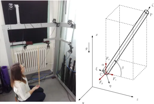
The goal is to determine the contact forces between the stick and the finger of the balancing person. In the measurement setup, which is shown in the left panel of Fig. 1. only the motion of the stick is measured. The mechanical model of the problem is depicted on the right hand side of Fig. 1. The stick is modeled as a homogeneous cylinder with radius r = 12 [mm], length l = 907 [mm] and mass m= 205 [g]. The mechanical model hasf = 5 degrees of freedom. To describe the motion we use the Cartesian-coordinates of the contact point C and two angles.
Therefore the vector of the generalized coordinates is q= [xC yC zC α β]|. We have m = 3 number of input forces τ = [Fx Fy Fz]|. These forces act in the contact point C. The coordinates which are constrained by the measurements are
ζ
ξ
η x
y
z α
β
Fy Fx
Fz
g
C
P
Fig. 1. The measurement setup and the mechanical model
the followings:
r(q) = rP
rCP
= rP
rP −rC
. (2.1)
Similarly to the so-called servo-constraint [13], the equation of motion has to constrained to the measurements as:
Er(q, t) =r(q)−rm(t) =0. (2.2) Herer(q) describes the constrained part of the motion as the function of the gen- eralized coordinates. The vector ofrm(t) describes the measured motion.
These servo-constraints cannot be satisfied precisely. Furthermore the measured values are geometrically inconsistent with the physical system because of the inac- curacy of the measurement. These inaccuracies could lead to numerical instabilities during the control force reconstruction. The stick balancing is an underactuated control problem, which means that it has more degrees of freedom than the number of actuator forces. Thus the servo-constraint based inverse dynamical computation is not unequivocal.
In this work we propose a new approach based on a predictive optimization process, which considers the whole recorded motion. The basic idea is inspired by the predictive control technique of underactuated manipulators [14] and [15]. In the
proposed technique, similarly to Eq. (2.2), an error vector is defined as:
E(q,q,˙ q, t) =¨
s0 r(q)−rm(t) s2 ¨r(q,q,˙ q)¨ −¨rm(t)
. (2.3)
As it can be seen,Eis extended by the errors on the level of acceleration. The gains s0ands2are used for weighting. In case of the presented problem these gains were set ass0= 1 ands2= 100.
These gains are needed because the measured values are not in the same order on the level of positions and accelerations. Using the error vector we define a cost function which have to be minimized:
Jhqi=
te
Z
t0
E|Edt. (2.4)
Here, the integral is calculated between t0 and te which define the time duration of the optimization problem. The integrand is the square of the norm ofE. In fact this cost function is a functional which depends on the generalized coordinates q.
The theory of calculus of variations [16] provides us tools to find the optimal time dependent functions of the generalized coordinatesqfor which this cost function is minimal.
The value of these generalized coordinates are not arbitrary because they have to be compatible with the solution of the equation of motion. It means that here the equation of motion is a second order non-holonomic constraint. These constrained problem is called an isoperimetric problem [16].
We assume that the equation of motion is written in the form
M(q)¨q+c(q,q) =˙ H(q)τ. (2.5) Here, we denote the mass matrix by M(q) ∈ Rf×f, the vector of the dynamical conditions and external forces is c(q,q)˙ ∈Rf, the independent actuator forces are denoted by τ ∈Rm and the distribution matrix of the actuator forces isH(q)∈ Rf×m.
As the mechanical model of the stick balancing is underactuated, it is possible to separate the equation of motion into two parts. The first equation is the actuated part as it contains the actuator forces τ, while the second one is the unactuated part as it does not depend on the actuator forces:
ga=Ma¨q+ca−τ =0, (2.6)
gu=Muq¨+cu=0. (2.7)
Herega ∈Rmandgu∈Rf−m. FurthermoreMaandMuare the appropriate parts of the mass matrix M(q). Similarly the vector c(q) is decomposed into two parts resulting the vectorsca andcu. From the first equation we can easily express the control forces, if we know the generalized coordinates, velocities and accelerations.
The second equationgu =0is actually the constraint from the viewpoint of the
generalized coordinates, since this equation does not involve the actuator forcesτ. The equationgu=0have to be satisfied as a constraint while calculatingqwhich results the closest solution to the measurement.
To find the optimal generalized coordinates first of all we have to define the Lagrange function L wherewith the Euler-Lagrange differential equations have to be expressed in the case of an isoperimetric problem [16]:
L=E|E+µ|gu, (2.8)
whereE|Eis the integrand of the cost functionJhqiandµ(t)∈Rf−mis a vector of unknown multipliers.
The Euler-Lagrange equations are defined with the functionLin the case of an isoperimetric problem. The optimization problem leads to the following system of ODEs:
∂L
∂q − d dt
∂L
∂q˙ + d2 dt2
∂L
∂¨q =0, (2.9)
gu=0. (2.10)
First of all we specify the initial values of the generalized coordinates and ve- locities att0:
q|˙ t0= ˙q0, (2.11)
q|t0=q0. (2.12)
We could also specify these at the end of the optimization problem (te).
In order to get a fully determined boundary condition problem at the end of the optimization timetethe following boundary conditions, which are called transver- sality conditions [16], have to be prescribed:
∂L
∂¨q
t
e
=0, (2.13)
∂L
∂q˙ − d dt
∂L
∂¨q
t
e
=0. (2.14)
3. Implementation of the optimization problem
The arising equations of the optimization problem are nonlinear differential equa- tions. These could be solved using numerical integration algorithms if all the bound- ary conditions were prescribed only at the beginning of the optimization (i.e., at time instant t0). However, the boundary conditions are not just at the beginning (timet0) but also at the end (timete) of the optimization. The numerical solution in this case is computationally expensive.
3.1. Linearization of the boundary condition problem
In order to overcome this problem, we can linearize the unactuated part of equation of motion (2.7) as:
gu≈αDq¨+βDq˙ +γDq+εD. (3.1) HereαD, βD, γD, δD, εDare constant matrices that can be produced using the following derivatives:
αD=∂gu
∂q¨ t
0
, (3.2)
βD=∂gu
∂q˙ t
0
, (3.3)
γD=∂gu
∂q t
0
, (3.4)
εD=−αDq|¨t0−βDq|˙ t0−γDq|t0. (3.5) This linearized form will provide acceptable solution only for a short time interval and the corresponding global optimization problem has to partitioned to local op- timization problems which have to be solved jointly. In other words, we consider a piecewise solution to the optimization problem. Thus the linearization has to be done only at the beginning of each sectiont0. Despite the partitioning requires the recalculation of the matrices at the beginning of each section, this approach is still numerically less demanding.
For faster computation it is beneficial to approximate the error vector too. For this, the measured coordinatesrm(t) have to be interpolated because the measure- ments provide a sequence of coordinates and not a continuous function, which is needed to get a solution in a closed form. The interpolation can be written in the following form:
rm(t)≈Prϕ, (3.6)
where ϕ contains trigonometric functions. In this paper we used the vector ϕ= [sin(α1t) cos(α1t) sin(α2t) cos(α2t)]|. Furthermore Pr is a constant matrix that can be determined with the least squares method. In the error vector defined in Eq. (2.3), the measured accelerations are also included. As the numerical dif- ferentiation of the measured values causes large noise it is better to calculate the accelerations in an analytic way using the interpolated position values. Thus the measured values in the error vectorEhave the following form:
s0rm
s2¨rm
≈Pϕ, whereP=
s0Pr
s2PrD2
. (3.7)
HereDis a differential operator which satisfies ˙ϕ=Dϕ.
We linearize the calculated coordinate valuesrand accelerations ¨rwith respect to the generalized coordinates q and their derivatives. These are included in the
error vectorEwhich can finally be written in the compact form:
E(q,q,˙ q, t)¨ ≈αE¨q+βEq˙ +γEq+εE−Pϕ. (3.8) Here the coefficientsαE,βE,γE andεE can be derived similar to the Eq. (3.1).
3.2. Solution of the linearized boundary condition problem
For the solution of the optimization problem the Euler-Lagrange (2.9) equation has to be expanded. Since the constraint equation (2.10) is a second order equation, the resulting differential equation will be a fourth order differential equation. Thus the boundary condition problem can be rewritten in the following form:
2α|EαEα|D αD 0
| {z } Ah1
q(IV)
¨ µ
+
U1,3 V1,1U1,2V1,0U1,1U1,0
U2,3 0 U2,2 0 0 0
| {z }
Ah0
...q
˙ µ
¨ q µ q˙ q
| {z } z
= Q
0
ϕ, (3.9)
where the sub-matrices can be calculated as:
U1,3= 2α|EβE−2β|EαE, (3.10)
U1,2= 2α|EγE−2β|EβE+ 2γ|EαE, (3.11)
U1,1=−2β|EγE+ 2γ|EβE, (3.12)
U1,0= 2γ|EγE, (3.13)
U2,3=βD, (3.14)
U2,2=γD, (3.15)
V1,1=−β|D, (3.16)
V1,0=γ|D, (3.17)
Q= 2α|EPD2−2β|EPD+ 2γ|EP−2γ|EεEKϕ,1. (3.18) Here, Kϕ,1 is a constant matrix for which Kϕ,1ϕ≈1. The derived equation is a system of inhomogeneous linear differential equation and it is solved in closed form using well known analytical methods. The homogeneous part of the equation have to be written in first order form and then the exponential solution is constructed.
In order to determine the particular solution of the inhomogeneous part we use the method of undetermined coefficients. Then, the sum of these two solutions will give us the general solution of the corresponding ODEs.
Solution of the homogeneous part of the equation
The homogeneous part of the linear ODE (Eq. (3.9)) is written in the following form:
˙
z=Ahz. (3.19)
The coefficientAh has the form:
Ah=
−A−1h1Ah0
I 0 0 0 0 0 0 I 0 0 0 0 0 0 I 0 0 0 0 0 0 0 I 0
, (3.20)
where I denotes the identity matrices of appropriate size. The solution can be expressed using a matrix exponential with a yet unknown constantCthat depends on the boundary conditions:
z=eAhtC. (3.21)
The particular solution of the inhomogeneous part of the equation
To get one of the solutions of the inhomogeneous part, we use the method of unde- termined coefficients and we assume that the solutions has the following form:
q=Pq,ihϕ, (3.22)
µ=Pµ,ihϕ. (3.23)
First, we substitute these and their time derivatives to the inhomogeneous part of Eq. (3.9). Next, we express the derivatives of ϕ using the differential operator matrixD. Finally, we collect the coefficients ofϕ, which contains the trigonometric functions of the interpolation. These coefficients must be equal on both sides of the derived equation, which leads to:
Ah1
Pq,ihD4 Pµ,ihD2
+Ah0
Pq,ihD3 Pµ,ihD Pq,ihD2
Pµ,ih
Pq,ihD Pq,ih
= Q
0
. (3.24)
This expression is a linear matrix equation which can be transformed into a system of linear equations.
Now the general solution of the optimization problem ODEs shown in Eq. (3.9) can be set up as the sum of the solution of the homogeneous and the inhomogeneous part:
q=Kq,0eAhtC+Pq,ihϕ, (3.25) µ=Kµ,0 eAht
C+Pµ,ihϕ, (3.26)
whereKq,0andKµ,0are the appropriate selector matrices, with which we can select theqandµvectors from z.
The equation of the boundary conditions
Since the equation gu =0is differentiated twice with respect to time in Eq. 3.9, two more boundary conditions have to be prescribed. It is arbitrary at which time instant we prescribe these conditions, but the time instantteis a reasonable choice:
gu|te =0, (3.27)
dgu dt
t
e
=0, (3.28)
From the general solution written in Eq. (3.25) and Eq. (3.26), we have to determine the exact solution corresponding to the boundary conditions (2.11)-(2.14) and (3.27)-(3.28). These lead to a system of linear equations with the unknown vectorC:
Abc,1
... Abc,6
| {z } Abc
C=
bbc,1
... bbc,6
| {z } bbc
. (3.29)
To derive the expression of the matricesAbc,i and bbc,i ; i= 1...6, we substitute the general solution (3.25) and (3.26) to the boundary conditions. Then, we collect the constants and the coefficients ofC. Therefore these matrices can be determined uniquely. Finally, the unknown constant vectorCis obtained as:
C=A−1bcbbc. (3.30)
Based on this, the generalized coordinates can be calculated using Eq. (3.25). Then the required actuator forcesτ is calculated from Eq. (2.6) as:
τ =Maq¨+ca. (3.31)
With these computed forces, the measured motion can be re-simulated based on the nonlinear equations of motion ( Eq. 2.5), and the results can be checked.
3.3. Numerical implementation
In order to derive analytical results, different approximations are used. We linearized the equation of motion and the error vector E (see: Eqs. (3.1) and (3.8)). This results in the fact that the outcome of the process is only acceptable over a short
∆tr time interval. On this time interval the results are used to re-simulate the motion. This means that we must solve a series of optimization problems during the force recalculation instead of only one. In the other hand to obtain a robust force recalculation we need to solve the optimization problem over a longer time interval called optimization time horizon.
Let us consider thei-th optimization illustrated in Fig. 2. The cost functionJhqi is minimized betweent0,iandte,i=t0,i+ ∆teafter which the equation of motion is
t0,i
tr,i=t0,i+1
te,i
t te,i+1
tr,i+1
∆tr
∆te
∆tr
∆te
Simulation interval: Optimization time horizon:
(i+ 1)-th section
i-th section
Fig. 2. Time intervals of the numerical resimulation
integrated using the calculated balancing forces betweent0,i and tr,i=t0,i+ ∆tr. This integration means that the original nonlinear equations of motion are solved by a numerical method. Finally the whole time horizon is moved forward by ∆tr
and the next (i+1)-th optimization process is started witht0,i+1=tr,i. It should be noted here that for the sake of clarity we used the notationst0=t0,iandte=te,i earlier.
4. Measurement results
The presented measurement was recorded by an Optitrack motion capturing system with the commercial software of Optitrack (see: left hand side of Fig. 1). The system measures the Cartesian coordinates of the centre points of the markers.
Table 1. Parameters of the measurement equipment
Marker type passive
Marker size 13 [mm]
Measurement frequency 120 [Hz]
Measurement accuracy 0.5 [mm]
During the measurement the movement of two inner points on the rod was recorded. Then the coordinates of the contact point C and the end point P were calculated with simple linear extrapolation. Therefore therC,m(t) andrP,m(t) func- tions are known. With these we can define the vector of the measured controlled coordinatesrm(t) similarly to Eq. (2.1).
Using the identification technique, the resulting balancing forces are shown in Fig. 3. Using the calculated forces, the equation of motion was re-simulated and
1.5 2 2.5
-0.5 0 0.5
0 5 10 15
-0.5 0 0.5
Fig. 3. The reconstructed contact forces
this way the measured and the simulated motion of the stick can be compared.
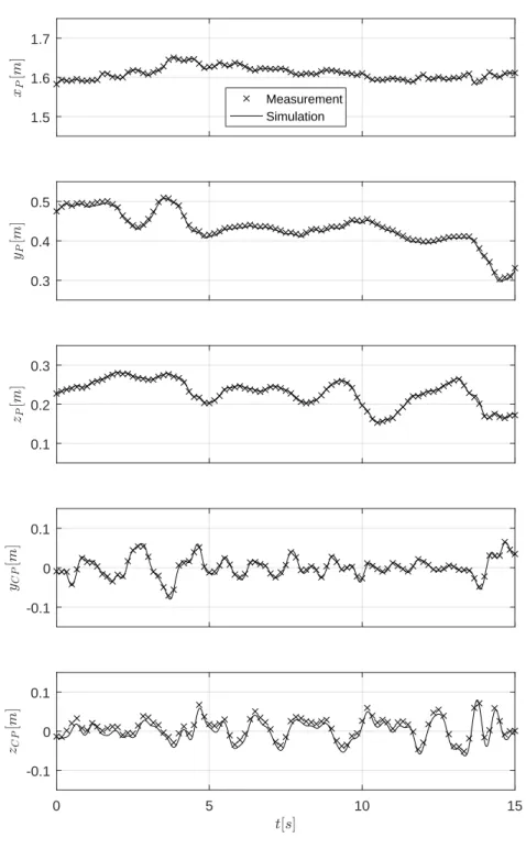
Fig. 4 shows that the recalculated values correspond well with the results of the measurements. The root mean square difference between the measurements and simulation was also calculated with the following formula:
RM S= v u u u t
1
∆t
∆t
Z
0
E|rErdt, (4.1)
where the integral is calculated on the whole time period [0, ∆t] of the resimulation.
As it can be seen in Fig. 4 ∆t= 15s. The calculated RMS value was 12.07mm.
This is the cumulated error of the measured and resimulated marker positions.
5. Conclusions
In order to understand human balancing processes the control forces have to be determined first. The aim of this study is to present a novel force recalculation approach for balancing problems. The goal is to find a control force which results a motion which is appropriately close to the recorded motion in case of a struc- turally unstable system. In this study for the investigation of the human balancing process, the problem of stick balancing was analyzed. For the control force recon- struction we have extended a predictive control technique. The numerical studies verify that the recalculated forces result very close motion with some accuracy to the recorded motion. The presented control force recalculation method will be used for identification of control of human balancing processes.
1.5 1.6 1.7
Measurement Simulation
0.3 0.4 0.5
0.1 0.2 0.3
-0.1 0 0.1
0 5 10 15
-0.1 0 0.1
Fig. 4. The measured and the simulated coordinates
Acknowledgments
The research reported in this paper was supported by ´UNKP-2017-2-1 New Na- tional Excellence Program of the Ministry of Human Capacities and the Higher Education Excellence Program of the Ministry of Human Capacities in the frame of Biotechnology research area of Budapest University of Technology and Economics (BME FIKP-BIO).
References
1. B. Mehta and S. Schaal, Forward models in visuomotor control, Journal of Neuro- physiology88(2002) 942–953.
2. G. Stepan, Delay effects in the human sensory system during balancing,Philosophical Transactions of the Royal Society A367(2009) 1195–1212.
3. T. Insperger and J. Milton, Sensory uncertainty and stick balancing at the fingertip, Biological Cybernetics108(1) (2014) 85–101.
4. J. Milton, R. Meyer, M. Zhvanetsky, S. Ridge and T. Insperger, Control at stabilitys edge minimizes energetic costs: expert stick balancing,Journal of the Royal Society Interface13(2016) p. 20160212.
5. P. Gawthrop, K.-L. Lee, M. Halaki and N. ODwyer, Human stick balancing: an in- termittent control explanation,Biological Cybernetics107(2013) 637–652.
6. J. G. Milton, T. Ohira, J. L. Cabrera, R. Fraiser, J. Gyorffy, F. K. Ruiz, M. A. Strauss, E. Balch, P. Marin and J. L. Alexander, Balancing with vibration: a prelude for.
7. N. Yoshikawa, Y. Suzuki, K. Kiyono and T. Nomura, Intermittent feedback-control strategy for stabilizing inverted pendulumon manually controlled cart as analogy to human stick balancing,Frontiers in Computational Neuroscience10(2016) p. 39.
8. G. C. Goodwin and R. Payne, Dynamic System Identification: Experiment Design and Data Analysis.(Academic Press, 1977).
9. www.optitrack.com, Optitrack motion capture system.
10. S. Whitaker and R. L. Pigford, An approach to numerical differentiation of experi- mental data,Industrial & Engineering Chemistry52(2) (1960) 185–187.
11. R. Kalman, A new approach to linear filtering and prediction problems,Journal of Basic Engineering1(82) (1960).
12. L. Bencsik, B. Bodor and T. Insperger, Reconstruction of motor force during stick balancing, in Proceedings of DSTA 2017: Engineering Dynamics and Life Sciences (Lodz, Poland, 2017), pp. 57–64.
13. W. Blajer and K. Ko lodziejczyk, A case study of inverse dynamics control of ma- nipulators with passive joints,Journal of Theoretical and Applied Mechanics (2014) 793–801.
14. L. Bencsik, L. Kov´acs and A. Zelei, Predictive trajectory tracking of underactuated systems,In proceedings of The 4th Joint International Conference on Multibody Sys- tem Dynamics(2016).
15. B. Bodor and L. Bencsik, Predictive control of robot manipulators with flexible joints, In proceedings of the 9th European Nonlinear Dynamics Conference(2017).
16. R. Weinstock,Calculus of variations1952.