E-CONOM
Online tudományos folyóirat I Online Scientific Journal
Főszerkesztő I Editor-in-Chief
KOLOSZÁR László
Kiadja I Publisher
Soproni Egyetem Kiadó I University of Sopron Press
A szerkesztőség címe I Address
9400 Sopron, Erzsébet u. 9., Hungary e-conom@uni-sopron.hu
A kiadó címe I Publisher’s Address
9400 Sopron, Bajcsy-Zs. u. 4., Hungary
Szerkesztőbizottság I Editorial Board
CZEGLÉDY Tamás HOSCHEK Mónika JANKÓ Ferenc SZÓKA Károly
Tanácsadó Testület | Advisory Board
BÁGER Gusztáv BLAHÓ András FARKAS Péter GILÁNYI Zsolt KOVÁCS Árpád LIGETI Zsombor POGÁTSA Zoltán SZÉKELY Csaba
Technikai szerkesztő I Technical Editor
TAKÁCS Eszter
A szerkesztőség munkatársa I Editorial Assistant
PATYI Balázs
ISSN 2063-644X
DOI: 10.17836/EC.2020.1.105
MOSER, Martin A.1
CAPM versus APT – two models in comparison
The classic portfolio theory deals with questions about the criteria that make up an optimal securities portfolio for a market participant and how it is composed. The Capital Asset Pricing Model (CAPM) forms the basis of modern financing theory. It was considered the key basic idea for the control and performance measurement of securities portfolios. In modern investment management, however, it has been increasingly replaced by multi-factor ap- proaches, such as the Arbitrage Pricing Theory (APT). The APT represents the second essential basic idea for the valuation of risky investment forms. This paper describes both models and compares the model assumptions, their practical suitability as well as advantages and disadvantages and an application example. Furthermore, the question is analyzed, which perspective Behavioral Finance brings and why this perspective is not covered in CAPM and APT models. The literature review was used as the method for processing the task.
Keywords: Capital Asset Pricing Model, Arbitrage Pricing Theory, portfolio theory JEL Codes: G11, G12, G41
CAPM versus APT – két modell ehhez képest
A klasszikus portfólióelmélet a piaci szereplők számára optimális értékpapír-portfóliót képező kritériumokkal és annak felépítésével kapcsolatos kérdésekkel foglalkozik. A tőkepiaci javak árazási modellje (CAPM) képezi a modern finanszírozási elmélet alapját. Ezt tartották az értékpapír-portfóliók ellenőrzésének és teljesítményméré- sének legfontosabb alapelvének. A modern befektetési menedzsmentben azonban azt egyre inkább felváltotta több tényezőjű megközelítés, például az arbitrázs árazási elmélet (APT). Az APT a kockázatos befektetési formák ér- tékelésének második alapvető ötlete. Az a cikk mindkét modellt leírja, és összehasonlítja a modell feltevéseit, azok gyakorlati alkalmasságát, valamint előnyeit és hátrányait, valamint egy alkalmazási példát. Ezenkívül azt a kérdést elemezzük, hogy a Viselkedési Pénzügy milyen perspektívát hoz és miért nem foglalkozik ez a perspektíva a CAPM és az APT modellekben. A feladat feldolgozásához irodalmi áttekintést használtam.
Kulcsszavak: tőkepiaci árfolyamok modellje, arbitrált árfolyamok elmélete, portfólióelmélet JEL-kódok: G11, G12, G41
Introduction
The aim of this paper is to process the main topic “CAPM versus APT – two models in com- parison” according to scientific criteria. Both models are presented, the model assumptions are compared, their practical suitability as well as advantages and disadvantages are given, and an application example of the two models is shown. Furthermore, the question has to be analyzed, which viewpoint brings Behavioral Finance and why this perspective is not covered in CAPM and APT models. Literature research should be used as a method for processing the task.
After the introduction, this paper first deals with the so-called portfolio theory. Following a general description of this topic, the following section on the Capital Asset Pricing Model (CAPM) already introduces a definition of the term, the practicality of this model, its ad- vantages and disadvantages and an application example. The next chapter is devoted to the second model dealt with, the Arbitrage Pricing Theory (APT), its definition, practicality, the advantages and disadvantages, as well as a brief application example. After the detailed de- scription and processing of both models based on an extensive and relevant literature search, the respective model assumptions are compared. The next chapter deals with and answers the
1 Ing. Martin A. Moser, MA MSc is PhD student at the University of Sopron, Alexandre Lamfalussy Faculty of Sopron, Hungary (martin.arnold.moser@phd.uni-sopron.hu).
above-mentioned question about behavioral finance. The last chapter briefly summarizes the most important and concise findings and results of this work.
Portfolio theory
The classic portfolio theory deals with questions about the criteria that make up an optimal securities portfolio for a market participant and how this portfolio is composed. The basis for the portfolio theory according to Markowitz is a stock market, which consists of a certain num- ber of securities and allows them to be put together individually. The grouping of various secu- rities is referred to as a portfolio (Markowitz, 1952:77–79.). It is assumed that each market participant makes a selection for the security portfolio from a certain number of securities. Sin- gle-period models, which are often referred to as market models, form the model framework of portfolio theory (Kremer, 2018:1.). The observation period is defined with a period and begins with a portfolio selection at the start time (t = 0). The initial equipment of the respective market participant and the prices on the market limit the investment decision. At the following point in time (t = 1), several environmental conditions can occur. At this point in time, every option for action entitles or obliges the respective decision-maker to make a payment that is dependent on the environmental status (Hüper, 2019:9.). This takes into account that the future development of the securities portfolio is subject to uncertainties (Kremer, 2018:1.).
The criteria by which market participants select security portfolios are decisive. Decision theory deals with the rules according to which rationally acting people make decisions and their behavior. The Bernoulli and the (µ, σ) criteria are the two most frequently used decision rules (Schmidt–Terberger, 1997:289.). The expected value of the future benefit of decision-makers is maximized according to the Bernoulli criterion (Bernoulli, 1738:177.). The assumption that market participants use the two indicators to assess security portfolios describes the (µ, σ) cri- terion according to Markowitz (Markowitz, 1952:77.). Portfolio theory implies that investors base their investment decisions solely on these two parameters. The yield is referred to as the expected value µ and the risk as the standard deviation σ. Within the scope of the portfolio theory, security portfolios are identified that generate a high return where possible for a given risk (Kremer, 2018:1.).
However, the two decision criteria mentioned above do not necessarily lead to the same result (Borch, 1969:3.). The Bernoulli and (µ, σ) criteria generally only result in the same se- lection of securities portfolios, if the distribution of portfolio returns is elliptical, which, how- ever, excludes financial goods with non-negative returns (Chamberlain, 1983:198-199.). In or- der to ensure that both criteria are valid at the same time, it can be assumed that the market participants have quadratic utility functions. Due to the fact that these indicate a higher actual risk aversion, this basic idea must be critically examined (Arrow, 1971:12.). The two criteria are now considered to be two different approaches to decision problems (Nielsen, 1990:226.).
In order to be able to define the properties of optimal securities portfolios more precisely, it must first be clarified according to which characteristics the market participants select them.
This requires a more precise description of the preferences of market participants. In this con- text, Markowitz assumes that investors are risk-averse, which means that two securities portfo- lios that have the same expected value but a different variance favor the one with the smaller variance. Conversely, it also implies that with the same variance but different expected values, the portfolio with the larger expected value is preferred (Markowitz, 1952:82.). In the course of portfolio theory, it is therefore assumed that investors have two specific properties that they identify as so-called rational investors. First, once an investor has the option of additional prof- its, they will realize them. Second, an investor will try to minimize the risks associated with the investment. This is known as risk aversion (Kremer, 2018:10-11.).
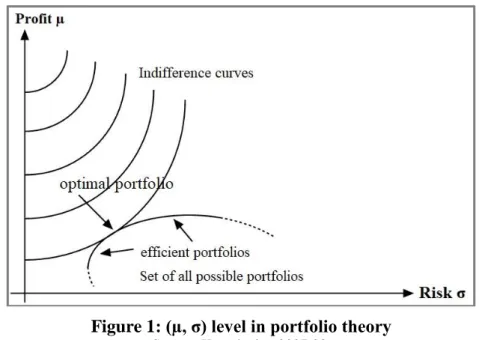
Figure 1 illustrates that the realizable securities portfolios with the lowest risk at the current expected value and the highest expected value at the current risk result in the number of efficient portfolios (Markowitz, 1952:82.). Which of these efficient securities portfolios is optimal for market participants depends on their preferences (Sharpe, 1970:52.). However, if a rational in- vestor has the choice between two investments in which the risk-return ratio is the same, then portfolio theory does not provide a basis for decision-making. In this case, the investor's risk attitude influences the selection of one of these investments (Kremer, 2018:11-12.).
Figure 1: (µ, σ) level in portfolio theory
Source: Kruschwitz, 2007:23.
To date, no assumptions have been made regarding the existence of a risk-free investment.
If it is assumed that a risk-free investment exists, this means that money can be invested and raised at a fixed interest rate. The combinations of risk-free and risky investments are in the (µ, σ) level on a straight line through both investments. A risk-free investment and investing in a risky security generate combinations between the two points. Taking out a loan and investing in the risky stock results in connections above the point that represents the risky investment. If a risky security portfolio is used instead of the risky security, the findings made are retained (Hüper, 2019:12.).
By integrating a risk-free investment, the efficient edge becomes a straight line that inter- sects the risk-free capital investment and touches the efficient edge of the risky security portfo- lios on the (µ, σ) level (Sharpe, 1970:67-68.). This risky portfolio of securities is called the tangential portfolio. All efficient portfolios consequently contain a linear combination of risk- free investment and tangential portfolio. The conclusion from this is that the optimal portfolio of a market participant results from the combination of risk-free capital investment and tangen- tial portfolio. There is therefore exactly one portfolio of securities, which consists of risky hold- ings and which all market participants hold. A market participant therefore only needs to know the tangential portfolio to put together the optimal securities portfolio. The selection of the risky security portfolio can therefore be seen as detached from the risk appetite of investors. In this context one speaks of the so-called separation theorem (Tobin, 1958:68.). The establishment of an investor's optimal equity portfolio only depends on the respective priorities (Hüper, 2019:12.).
The return on a securities portfolio, as well as the variance of the portfolio return, result from the linear combination of the returns of the financial instruments contained in each case.
The observed effect of diversification illustrates that a suitable mix of financial stocks in the
securities portfolio can reduce its risk without reducing the expected return equally (Kremer, 2018:14.).
If a variety of risky securities is supplemented by a risk-free investment, efficient security portfolios can be easily presented. The next chapter is dedicated to the Capital Asset Pricing Model (CAPM), according to which the efficient portfolios are located on the so-called capital market line, which can be represented as a straight line in the (µ, σ) diagram (Kremer, 2018:32.).
Capital Asset Pricing Model
Definition
The Capital Asset Pricing Model (CAPM) was developed in the 1960s by Sharpe (Sharpe, 1964:425–427.), Lintner (Lintner, 1965:13–15.) and Mossin (Mossin, 1966:768–770.) and rep- resents in its different variations a basis of modern financing theory. It is a balance model and developed from the objective to explain the pricing and thus the income of alternative invest- ments (Warfsmann, 1993:1.). It deals with the question of how the portfolio risk can be deter- mined and the relationship between expected return and risk (Hüper, 2019:1.).
The foundation stone for the derivation of the CAPM is formed by the portfolio theory of Markowitz (Markowitz, 1952:77–79.) and the separation theorem by Tobin (Tobin, 1958:65- 67.). The decision criterion is the (µ, σ) criterion formulated by Markowitz and described at the beginning (Markowitz, 1952:77.). By examining the investment behavior of a reasonably- priced, risk-averse investor, it can be concluded that the investor chooses a security portfolio solely on the basis of the expected return and variance. Given the risk, investors only hold the portfolio that delivers the highest expected return. Since there is a different efficient portfolio for each risk, there are an unlimited number of efficient portfolios (Warfsmann, 1993:1.). Tobin claims that if a risk-free security exists, each efficient equity portfolio is only a compilation of two efficient portfolios (Tobin, 1958:65–67.).
As a result, the CAPM shows that there is a linear relationship between the valuation- relevant risk and the expected return in equilibrium. The former is expressed by the so-called beta value (risk indicator) (Hüper, 2019:1.). This model is based on several market assumptions and some other assumptions about individual market behavior. The assumptions in the market are usually that the markets are smooth (no transaction costs, no taxes, etc.). In addition, it is assumed that there is a risk-free asset (Wilhelm, 1985:6.).
In the meantime, the expansion of the CAPM to the multi-period case has also been ex- amined in the literature. For example, Fama considers a model world with several periods and discrete times. It shows that with continuous investment opportunities, an extension of this model to the multi-period case can be carried out and that the findings for the one-period case remain valid in the multi-period case (Fama, 1970:165-166.). Merton looks at continuous points in time and examines the phenomenon of constant and non-constant opportunities for capital investment (Merton, 1973:875.). The different variants for the multi-period case, which have been dealt with in the literature to date, have in common that, in addition to the (µ, σ) criterion, an expected maximization of benefits is assumed as a further decision-making feature. The assumptions made in the one-period case are based only on the (µ, σ) criterion as a decision criterion (Hüper, 2019:2.).
The design of the decision criterion plays an important role. In addition to the original form of the (µ, σ) criterion according to Markowitz, the characteristic of the variance version was established by Duffie. It shows that the assumption of variance aversion and strict uni- formity in risk-free capital investments instead of the (µ, σ) criterion also prove the CAPM (Duffie, 1988:95–97.). These two criteria were initially regarded as weaker assumptions in the literature. However, Löffler has proven that both assumptions can be regarded as equivalent in the one-period case (Löffler, 1996:534-535.).
In addition to the traditional CAPM, there is also the Tax-CAPM, the CAPM with incom- plete information according to Merton (1987), as well as the liquidity CAPM according to Kempf (1999) and Jacoby / Fowler / Gottesman (2000), due to the limited scope of the paper this will not be discussed in detail.
Practicality
Although the classic CAPM was first designed several decades ago, it has not lost its importance even today. Due to its relatively manageable design, it can be used in theory and practice in different situations. As an equilibrium model, its claims refer to various investment opportuni- ties (Warfsmann, 1993:1.). When examining the CAPM with a variety of test methods, it was found that the results obtained are significantly influenced by the selection of the test method (Stambaugh, 1982:241-243.).
Nevertheless, the CAPM is constantly criticized (Ballwieser, 2008:105.). As mentioned in the previous chapter, the classic CAPM is a one-period model. In the first moment, a selection is made and in the second, the risk is realized, because of which investments, savings or con- sumption are made. This variant of the CAPM is probably one of the most commonly used economic theories. Nevertheless, this type of model cannot adequately represent reality. Robert Merton's so-called intertemporal CAPM tries to fix this. In this model, the actors can act at any time. If this is assumed, a model can be constructed mathematically, which is regarded as a basic generalization of the one-period CAPM (Hüper, 2019:VII.). This is essential for the prac- ticality of CAPM, since valuation questions in the context of company valuation often represent problems in a multi-period context. It is therefore necessary to extend the original one-period model to the multi-period case. At the beginning of each phase, market participants have to make an investment and consumption decision. They allocate the assets from their previous investment strategy to the acquisition of a new security portfolio and a withdrawal. Decision rules must be laid down according to which market participants make these decisions (Hüper, 2019:5.).
The addition of the classic CAPM to the multi-period case is of particular importance for evaluation questions. For example, Fama describes that under the idea of continuous investment opportunities, an expansion of the CAPM to the multi-period case can be achieved. One speaks of continuous investment opportunities if the allocation of future income is independent of the respective environmental status (Fama, 1970:171-172.). In this case, the CAPM hypotheses remain valid. The linear link between expected return and systematic risk of a securities port- folio, which is characterized by the securities market line, remains intact. If the investment opportunities are not continuous, this is not the case. Stapleton and Subrahmanyam consider stochastic returns as opposed to processes for returns (Stapleton–Subrahmanyam, 1978:1082- 1083.). The case of non-continuous investment opportunities is also considered by Constan- tinides, among others (Constantinides, 1980:77–79.).
Furthermore, the classic CAPM ignores personal contributions from shareholders in its original form. This suggests that market participants are undecided between earnings and profit distributions. The taxation of capital and interest income, as well as profit distributions, is often done in different ways. This can lead to two securities portfolios with the same pre-tax returns having different after-tax returns due to the different separation of investment income, interest income and profit distributions (Hüper, 2019:3.). In order to illustrate the importance of per- sonal taxes in this model world, the so-called Tax-CAPM was developed (Brennan, 1970:421.).
Taxes are determined and paid, but these subsequently disappear from the model. The use or whereabouts of the taxes is not explained in more detail. To remedy the problem, Kruschwitz and Löffler extend the model by redistributing tax revenues to market participants and describe the existence of equilibrium prices under certain hypotheses that remain the same if the tax rate changes (Kruschwitz–Löffler, 2009:174-175.).
In addition, the dependence of this model on the market portfolio is criticized, which in reality is difficult to define and in practice is not held by all market participants (Hüper, 2019:17.). Furthermore, the path of risk-free investment and taking out a loan at an interest rate that is identical for all market participants is not available in reality (Hüper, 2019:18.). Another problem is the use of the (µ, σ) criterion as a basis for decision-making, which is only compat- ible with the Bernoulli criterion in special cases (Schmidt–Terberger, 1997: 297-298.). Finally, the missing costs for transactions, the assumption of the same ideas of the market participants as well as the lack of empirical recognition regarding the assessment of the practicality of this model should be mentioned (Kruschwitz, 2007:227.).
Nevertheless, in reality the CAPM is a widely used valuation model. The Institute of Accountants (IDW) suggests using the model, for example, to raise the capitalization interest rate in the course of company valuations (IDW, 2014:108.).
Advantages and disadvantages
The advantages of the CAPM lie in its simple and user-friendly theoretical structure (Warfs- mann, 1993:3.), as well as the assumption that investors hold a diversified portfolio of secu- rities, since this can eliminate specific risks (Vollmer, 2015:21.). Furthermore, the CAPM takes into account the beta value (systematic risk), which is unforeseen and often cannot be completely mitigated, since it is often not fully expected (Schuster–Uskova, 2015:162.). If the business mix and the financing of a company differ from the current business, then other required methods or models for calculating the return cannot be used, but CAPM can (Stahl, 2016:13–15.).
Disadvantages of the CAPM are found on the one hand in the occurrence of a large num- ber of statistical problems in the empirical review, on the other hand this model does not refer to the actual yields that can be determined in practice, but to the assumed yields at the time of the decision (Warfsmann, 1993:3.). Furthermore, the CAPM can only explain the yields insuf- ficiently, although the relationship between higher beta value and higher yield is confirmed in empirical work (Black et al., 1972:79–81.). Making assumptions leads to standard econometric problems and there is a possibility of errors in the variables and the existence of nonlinear hy- potheses (Warfsmann, 1993:3.). Furthermore, the use of the generally accepted interest rate is a disadvantage or a problem of the CAPM, since the yield changes daily and creates volatility (Vollmer, 2015:21.). In reality, the assumption that investors can take out and lend loans with- out risk is unrealistic and unreachable (Vollmer, 2015:21.).
Companies that use CAPM to evaluate an investment must find a security risk that relates to the project or investment, whereby an exact identification of the project is difficult and can affect the reliability of the result (Schlegel, 2015:13.). Another disadvantage of the CAPM is the necessity to question the entire methodology for determining the risk-free interest rate due to conceivable mispricing (Elsner–Krumholz, 2014:350–352.). It is contested that the CAPM cannot be validated empirically, since the market portfolio cannot be determined directly (Roll, 1977:129–131.). Despite the investigation of the US stock market, the fundamental difficulty of the short-term instability of the beta value is becoming noticeable (Kern–Mölls, 2010:440–
442.). There is criticism that the calculation of the beta value for individual investments is less precise than for securities portfolios (Scheld, 2013:108.).
Application example
The security risk is also known as the beta value. As previously explained theoretically, the higher the beta value of an investment, the higher the expected return. Accordingly, investors want to be compensated for the risk to be borne by a higher return. The beta value is also used as a risk indicator for individual companies (Schuster–Uskova, 2015:162.).
Table 1: Beta values of shares A to E
Share A B C D E
Beta value 0.70 1.00 1.15 1.40 – 0.30
Source: Schuster–Uskova, 2015:163.
In this application example, which is intended to clarify the practical use of the CAPM, a risk-free interest rate of 5% and an expected market return of 9% are assumed. The expected return of the respective share is then calculated from table 1 (Schuster–Uskova, 2015:163.).
Expected return = Risk-free interest rate + Beta value * (Market return – Risk-free interest rate) Expected return of share A = 0.05 + 0.70 * (0.09 – 0.05) = 0.078 = 7.8%
Expected return of share B = 0.05 + 1.00 * (0.09 – 0.05) = 0.090 = 9.0%
Expected return of share C = 0.05 + 1.15 * (0.09 – 0.05) = 0.096 = 9.6%
Expected return of share D = 0.05 + 1.40 * (0.09 – 0.05) = 0.106 = 10.6%
Expected return of share E = 0.05 – 0.30 * (0.09 – 0.05) = 0.038 = 3.8%
It can be seen that the larger the beta value of the respective security, the greater the risk- adjusted return on earnings. The CAPM states that all possible securities portfolios are on the so-called securities line, since the market is balanced and information-efficient. The security line shows the return requirement depending on the risk of individual securities. This means that all investments above the security line are undervalued and therefore give a buy signal.
Conversely, investments that are below the securities line are overvalued and should be sold (Schuster–Uskova, 2015:161–163.).
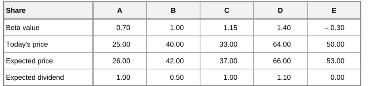
Table 2: Shares A to E incl. today’s/expected price and dividend
Share A B C D E
Beta value 0.70 1.00 1.15 1.40 – 0.30
Today's price 25.00 40.00 33.00 64.00 50.00
Expected price 26.00 42.00 37.00 66.00 53.00
Expected dividend 1.00 0.50 1.00 1.10 0.00
Source: Schuster–Uskova, 2015:164.
In order to identify the undervaluation or overvaluation, the required yield is then com- pared with that expected in the future. For this purpose, the return on capital gains (= (expected price – today's price) / today's price), the dividend yield (= expected dividend / today's price) and the estimated total return in % (= return on capital + dividend yield) are calculated (Schus- ter–Uskova, 2015:164.).
Table 3: Shares A to E incl. calculated characteristic values
Share A B C D E
Beta value 0.70 1.00 1.15 1.40 – 0.30
Return on investment 4.00 5.00 12.12 3.13 6.00
Dividend yield 4.00 1.25 3.03 1.72 0.00
Estimated return 8.00 6.25 15.15 4.84 6.00
Expected return 7.80 9.00 9.60 10.60 3.80
Difference 0.20 – 2.75 5.55 – 5.76 2.20
Source: Schuster–Uskova, 2015:164.
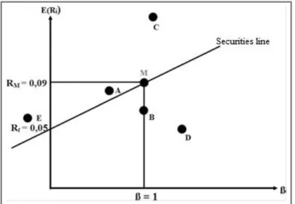
Figure 2 shows the values entered in the CAPM. It can be seen that shares A, C and E are undervalued and B and D are overvalued. The CAPM states that all investments and securities portfolios are on the securities line (Schuster–Uskova, 2015:165.).
Figure 2: Estimated and expected return on shares A to E
Source: Schuster–Uskova, 2015:165.
The CAPM was considered the key basic idea for the control and performance measure- ment of securities portfolios, as well as for determining the cost of capital. In modern invest- ment management, however, the CAPM has been increasingly replaced by multi-factorial ap- proaches, such as the Arbitrage Pricing Theory (APT) (Rösch, 1998:223.).
Arbitrage Pricing Theory
Definition
The Arbitrage Pricing Theory (APT) developed by Ross was first presented in the Journal of Economic Theory in 1976 (Ross, 1976:341–343.). In addition to the CAPM, it represents the second essential basic idea for the valuation of risky forms of investment. In the meantime, a large number of approaches have existed in the literature since Ross's first assumption, some of which differ greatly in the model assumptions, but are nowadays referred to as APT (Rösch, 1998:V.). The model emerged from the previously criticized points of the CAPM and represents
a further instrument for determining the cost of equity (Pankoke–Petersmeier, 2009:129.). In- stead of a market equilibrium, arbitrage-free markets are assumed. The term arbitrage describes the use of price or price differences in different markets (Perridon et al., 2012:289-290.). Ross thus implies homogeneous expectations of investors, because on this basis adjusted prices for equivalent ratios of income and risk are formed and consequently arbitrage opportunities are isolated (Volkmann, 2005:52-53.).
The starting point of the APT is the so-called factor model, which is intended to fully describe the yield-generating market process. The economic idea behind this model is that the non-diversifiable security risk can be described by a few elementary factors (Garz, 2000:254.).
Basically, the APT is a generalization or further development of the approach in which a market balance is described by the fact that the price of a share corresponds to the price of a linear combination of elementary securities that simulate the condition-dependent payment flow of the traded share (Debreu, 1959:83.).
The APT is essentially a multi-factor model that attempts to describe the return on assets and their covariance matrix as a function of a limited number of risk attributes (Dhankar, 2019:19.). Instead of a risk factor, APT uses various factors to describe the decisive return on securities (Pankoke–Petersmeier, 2009:129.). These risk factors can be determined both from historical returns and from macroeconomic variables (Sauer, 1994:94-96.). The view of the linear relationship between income and risk remains unchanged (Grimm et al., 2014:266.). The division of systematic and unsystematic risk is also being pursued (Hofbauer, 2011:73.). The type and number of risk factors is not restricted (Pankoke–Petersmeier, 2009:129). The differ- ent risk influences are determined by means of specific, linear regression coefficients (beta factors) for the respective investment under consideration (Stahl, 2016:25.).
Other prerequisites and assumptions are reasonable investors and the disregard of taxes and transaction costs. Furthermore, APT also assumes that investors can invest and borrow unlimited funds at a risk-free interest rate. The fact that a normal distribution of earnings is not assumed and that the market portfolio has no significance shows that APT is subject to less restrictive assumptions (Copeland et al., 2008:244.).
Practicality
Since the selection of risk influences at APT is partly based on subjective assessments (Volkmann, 2005:53.), an empirical model review and its application in practice are not easy (Wallmeier, 1997:82.). When APT is used in practice, there is a risk that assumptions similar to CAPM must be made again to define the parameters (Lockert, 1998:75.). A small number of factors are stated to be suitable, although the teaching is disagreed and the number sometimes exceeds the single-digit range (Roll–Ross, 1980:1077.).
Furthermore, the ongoing historical data for the determination of the regression coeffi- cients and influences of the risk with regard to the choice of the observation period and interval as well as the general use of historical data are criticized (Grimm et al., 2014:267.). The use of cross-sectional regressions can lead to the determination of insignificant risk influences due to the inherent unsystematic risks and the resulting distortion (Hamerle–Rösch, 1998:38–40.). Due to the difficulties and disadvantages mentioned above and below, APT has so far not been able to establish itself in practical application in company valuation practice (Pankoke–Petersmeier, 2009:129.). A precise design of the additional risk factors takes place, for example, in the so- called 3-factor model, which, however, will not be dealt with in more detail in the course of this paper (Hanauer et al., 2013:4.).
Advantages and disadvantages
The advantages lie in its multi-dimensionality of the risk factors, which allows more flexible modeling and a more differentiated insight into the risk structure of investments (Pankoke–
Petersmeier, 2009:129.). On the other hand, it offers better economic interpretability of the re- sults, if the risk factors are specified in advance, such as the expected inflation (Vogler, 2009:384-385.). Furthermore, the ATP offers better empirical testability of the results, since the market portfolio does not play a role, unlike the CAPM. Due to the higher explanatory content, this model delivers better empirical test results overall (Grimm et al., 2014:267.).
A disadvantage of APT is the fact that the various risk factors do not guarantee a homo- geneous and understandable result. The influences of the risks are therefore not determined by the model and there is no relief with regard to the quantity of the risk parameters, which can lead to so-called pseudo-correlations (Hachmeister, 2000:227.). The use of the APT requires the user to conduct an uneconomical investigation and to select the required factors (Pankoke–
Petersmeier, 2009:129.). Another disadvantage of APT as a multi-factor model is seen in the lack of microeconomic anchoring, which Ross, in turn, considers to be unnecessary (Hachmeis- ter, 2000:227.). In his opinion, knowledge of the risk factors that influence the specific return is sufficient (Vogler, 2009:384-385.).
Application example
The APT states that the expected return on a security must correspond to the following relation (Hens–Rieger, 2016:182-184.).
Expected return = r(f) + b(1) * rp(1) + b(2) * rp(2) + … + b(n) * rp(n)
r(f) … risk-free interest rate
b … Condition of the asset for the particular factor rp … Risk premium for the specific factor
The number of risk factors depends on the examination, i.e. which factors an analyst chooses and considers relevant. The factors need not be the same across all analyzes. For the application example shown here, it is assumed that a stock is being examined. Exemplary risk factors have been identified, including their inventory sensitivity and the associated risk pre- mium (Hens–Rieger, 2016:182–184.).
Risk free interest rate: r(f) = 3%
Gross domestic product growth: b = 0.6 rp = 4%
Inflation rate: b = 0.8 rp = 2%
Gold prices: b = – 0.7 rp = 5%
S&P 500 Index Return: b = 1.3 rp = 9%
As an index, the S&P 500 tracks the securities of the 500 largest listed US companies and is weighted according to market capitalization. The expected return is now calculated using the formula given at the beginning of the example (Hens–Rieger, 2016:182–184.).
Expected return = 3% + (0.6 * 4%) + (0.8 * 2%) + (– 0.7 * 5%) + (1.3 * 9%) = 15.2%
Comparison of the models
The CAPM is an equilibrium model that explains why different securities have different ex- pected returns. It provides a method to quantify the risk and translate that risk into estimates of the expected return on equity. In particular, it is claimed that expected returns vary because securities have different beta values. There is a linear relationship between beta value and ex- pected return. The alternative asset pricing model, APT, on the other hand, assumes that returns on securities are generated by a factor model, but does not identify the factors. This implies that
securities or portfolios with the same sensitivities should offer the same expected returns. If not, investors will take advantage of arbitrage opportunities and have them eliminated. The expected equilibrium return of a security is a linear function of its sensitivity to the factors (Dhankar, 2019:20.). According to different empirical studies, the APT guarantees a higher explanatory content than the CAPM (Pankoke–Petersmeier, 2009:129.).
The assumption of a balance on the capital market and the recourse to the unobservable market portfolio and benefit theory strategies are often seen as disadvantages of the CAPM.
Conversely, it must be recognized that the lack of these hypotheses, contrary to the exact as- sessment equation of the CAPM, does not allow an exact assessment of the factors. If an accu- rate assessment that is related to the CAPM is to be achieved solely through systematic dangers, then reference must be made to the assumption of equilibrium on the capital market and to benefit theory. Apart from the factor model assumption, the derived models differ only mini- mally from the CAPM in their acceptance catalogs (Rösch, 1998:345.).
A combination of both models forms the equilibrium APT (Chen–Ingersoll, 1983:985- 986.). Here the assumption of a factor model of the APT is combined with the objective function of maximizing the expected benefits of the CAPM. This means that the renunciation of more specific preference assumptions, which was originally considered to be a major advantage of the APT, is lost. Conversely, however, the chance is gained to be able to find stricter explana- tions regarding the assessment of the factors (Garz, 2000:255.).
If the relationship between the CAPM and the APT is examined in more detail, it can be seen that frequently made statements regarding the higher general validity of the APT (Bur- meister et al., 1994:312.) or that it should be less restrictive should not be considered without a more precise analysis (Rösch, 1998:344.). A real additional assumption is the dependence of the return on securities on economic risk factors. The CAPM does not require this assumption (Treynor, 1993:11.). The APT, on the other hand, requires the existence of a factor model (Sharpe, 1984:23.). However, this is not intended to suggest that such a factor structure is not permitted by the CAPM (Gilles–LeRoy, 1991:226.).
Behavioral Finance
Definition
Behavioral Finance is a subject area of Behavioral Economics, which deals with human behav- ior in different economic situations, describes the difference between the behavior of investors adopted and described in classic capital market theory and the behavior that can be observed in reality. Classic capital market theory has certain weaknesses, such as the illogical behavior of investors. Behavioral finance tries to identify and explain repetitive schemes in this behavior.
The first approaches to this appeared in the United States in the 1960s. Pioneers in this area were primarily Daniel Kahneman and Amos Tversky, as well as Richard Thaler (Kitzinger, 2013:17.).
In addition to illogical acting, the different nature of investors' views and inclinations are among the recurring topics. As a result, the valuations of individual investors' assets deviate massively from the fundamental value. This influence creates arbitrage opportunities for those investors who understand and predict the systematic deviations (Averbeck, 2010:13–15.). In contrast to fundamental analysis, the technical analysis of price trends does not attempt to de- termine the intrinsic value of a security, but rather notes on future developments from price trends and the associated trends are taken (Murphy, 2004:218-219.).
Whenever it is necessary to examine deviations from completely rational behavior, one speaks of behavioral finance. It is therefore obvious that a clear distinction between problems inside and outside behavioral finance is impossible. There are situations in which investors mostly behave rationally. However, this is not always the case, so that a simple model can be
successful if only rational behavior is taken into account, but appropriate corrections have to be made when taking a closer look (Hens–Rieger, 2016:11.).
According to the classic definition of Fama (1970), an efficient market is a market in which the prices always fully reflect the information available. The market prices contain in- formation both about events that have already occurred and about events that the market is now expecting for the future (Fama, 1970:164–166.).
Depending on the amount of information that should be reflected in asset prices, there are three basic forms of information efficiency in the capital market. Weak efficiency presupposes that stock prices reflect all important information from historical pricing. Investors cannot pre- dict how asset prices will behave in the future solely due to price changes in the past. The semi- powerful efficiency increases the amount of information that is taken into account when pricing assets. It is believed that stock prices not only reflect the information that can be obtained from historical prices, but also all other publicly available information such as company accounts or profit forecasts. After all, high efficiency means that information, regardless of whether it is public or private, confidential and available to a small group of people, is only quickly reflected in share prices if it can be induced by observing insider actions (Szyszka, 2013:27.).
Markets can remain efficient, even if not all investors are rational and some of them make mistakes in perceiving and responding to information. In such a case it is assumed that irrational investors act randomly in the market. If their trading decisions are not correlated, their effects are likely to cancel out. Overall, they will not generate market power that could affect equilib- rium prices. Your transactions only increase the trading volume. This argument is crucially based on the lack of correlation in the behavior of irrational investors (Szyszka, 2013:28.).
Connection with financing models
Behavioral finance naturally questions all the assumptions mentioned above and the hypothesis of market efficiency. The human mind is often imperfect in how it perceives reality and pro- cesses information. Investors cannot correctly value securities and their preferences can change for no reason. Irrational behavior is far from individual. It is often shared by certain groups of investors, which can lead to regular problems with correct pricing. Market participants, includ- ing rational ones, can show symptoms of so-called herd behavior by receiving information, observing others and underestimating the results of their own analyzes. As a result, they copy the measures taken by others so that the market does not reflect part of the private information that is known to its actors. In extreme cases, investors may not be in the least bit interested in finding and processing basic information about companies, taking a purely speculative ap- proach. They buy certain securities not because they are motivated by a rationally calculated ratio of risk and expected return, but mainly because they expect other market participants to rate the same instruments even higher in the near future. With this approach, the current market prices can of course differ from the actual value of the securities. Even if rational arbitrageurs will have no problem noticing such deviations from correct pricing, they will not always be able to actively participate and bring prices back to their fundamentals. The reason for this is that even rational investors are often faced with restrictions that do not allow them to benefit from the mispricing they have identified (Szyszka, 2013:29.).
Although behavioral finance provides explanations for why people make biased deci- sions in situations of uncertainty, it is difficult to incorporate this qualitative knowledge into models such as the CAPM and the APT. Fama and French were among the most prominent defenders of market efficiency and the forerunners of multi-factor models. They argue that the anomalies are risk factors that can be included in and explained by larger models. Propo- nents of behavioral finance, however, blame prejudices, emotions and affects for many anom- alies (Jordan, 2004:10–12.).
Summary
Knowing the expected returns on a security before investing is important for shareholders, in- vestors and financial experts alike. There are various assessment tools for this.
The Capital Asset Pricing Model (CAPM) and the Arbitrage Pricing Theory (APT) are tools for pricing assets. The CAPM assumes that there is a capital market balance. In contrast to the CAPM, the APT also allows several factors and does not require a market balance, but only an arbitrage-free securities market. The main advantages of the CAPM are the simple structure and the adoption of a diversified portfolio of securities. Disadvantages lie in statistical problems in the empirical review and inadequate explanation of returns. The main advantages of APT are its multidimensionality and better empirical testability. A major disadvantage is that the clearly imaginable risk factors cannot guarantee a clear result.
Both models assume that investors act rationally. Behavioral finance deals with human behavior in different economic situations and describes the difference between the behavior of investors assumed in classic capital market theory and the behavior that can actually be ob- served in reality. The psychological effects associated with behavioral finance show that the assumptions underlying the CAPM and APT cannot be maintained in practice. This does not mean that the findings of the models that apply intuitively should be completely rejected. How- ever, it is necessary to integrate a psychological component into the models, since the consid- erable influence of the human psyche on course formation cannot be denied.
References
Arrow, K. J. (1971): Essays in the Theory of Risk-Bearing. Chicago: Markham Publishing Company.
DOI: 10.2307/2978877.
Averbeck, D. (2010): Die Rolle der Behavioral Finance bei der Preisbildung an Aktienmärkten: Im- plikationen für die Entstehung von Spekulationsblasen. Saarbrücken: VDM Verlag.
DOI: 10.1007/978-3-662-55924-6_2.
Ballwieser, W. (2008): Betriebswirtschaftliche (kapitalmarkttheoretische) Anforderungen an die Un- ternehmensbewertung. WPg Sonderheft, Pages 102–108. DOI: 10.1007/978-3-322-84076-9.
Bernoulli, D. (1738): Specimen theoriae novae de mensura sorties. Commentarii Academiae Scientiarum Imperialis Petropolitanae, Pages 175–192.
Black, F. – Jensen, M. C. – Scholes, M. (1972): The Capital Asset Pricing Model: Some Empirical Tests. Studies in the Theory of Capital Markets, Pages 79–121.
Borch, M. (1969): A Note on Uncertainty and Indifference Curves. The Review of Economic Studies, Pages 1–4. DOI: 10.2307/2296336.
Brennan, M. (1970): Taxes, Market Valuation and Corporate Financial Policy. National Tax Journal, Pages 417–427.
Burmeister, E. – Roll, R. – Ross, S. A. (1994): A Practitioner’s Guide to Arbitrage Pricing Theory. Fi- nanzmarkt und Portfolio Management, Volume 8, Pages 312–331.
Chamberlain, G. (1983): A characterization of the distributions that imply mean-variance utility func- tions. Journal of Economic Theory, Pages 185–201.
DOI: 10.1016/0022-0531(83)90129-1.
Chen, N. – Ingersoll, J. (1983): Exact pricing in linear factor models with finitely many assets: a note.
Journal of Finance, Volume 38, Pages 985–988. DOI: 10.1111/j.1540-6261.1983.tb02512.x.
Constantinides, G. M. (1980): Admissible Uncertainty in the Intertemporal Asset Pricing Model. Jour- nal of Financial Economics, Pages 71–86. DOI: 10.1016/0304-405x(80)90022-7.
Copeland, T. E. – Weston, J. F. – Shastri, K. (2008): Finanzierungstheorie und Unternehmenspolitik:
Konzepte der marktorientierten Unternehmensfinanzierung. (4. Auflage). München: Pearson Deutschland GmbH. DOI: 10.1524/9783486811483.171.
Debreu, G. (1959): The Theory of Value: An Axiomatic Analysis of Economic Equilibrium. New Ha- ven and London: Yale University Press. DOI: 10.2307/1055180.
Dhankar, R. S. (2019): Risk-Return Relationship and Portfolio Management. New Delhi: Springer Na- ture India Private Ltd. DOI: 10.1007/978-81-322-3950-5.
Duffie, D. (1988): Security Markets, Stochastic Models: Economic Theory, Econometrics, and Mathe- matical Economics. New York: Academic Press, Inc. DOI: 10.2307/2328286.
Elsner, S. – Krumholz, H.-C. (2014): Eine Anmerkung zur Bestimmung des Basiszinses in der Unter- nehmensbewertungspraxis: Eine Schätzung benötigt keine Staatsanleihen. Corporate Fi- nance, Volume 9/2014, Pages 350–360.
Fama, E. F. (1970): Multiperiod Consumption-Investment Decisions. The American Economic Re- view, Volume 60, Pages 163–174. DOI: 10.1016/b978-0-12-780850-5.50035-6.
Garz, H. (2000): Prognostizierbarkeit von Aktienrenditen: Die Ursachen von Bewertungsanomalien am deutschen Aktienmarkt. Wiesbaden: Springer Fachmedien GmbH.
DOI: 10.1007/978-3-663-08180-7.
Gilles, C. – LeRoy, S. F. (1991): On the Arbitrage Pricing Theory. Economic Theory, Volume 1, Pages 213–229. DOI: 10.1007/bf01210561.
Grimm, R. – Schuller, M. – Wilhelmer, R. (2014): Portfoliomanagement in Unternehmen. Wiesbaden:
Springer Gabler Verlag. DOI: 10.1007/978-3-658-00260-2.
Hachmeister, D. (2000): Der Discounted Cash Flow als Maß der Unternehmenswertsteigerung. (Dis- sertation, 4. Auflage). Frankfurt am Main: Lang Verlag.
Hamerle, A. – Rösch, D. (1998): Zum Einsatz „fundamentaler“ Faktorenmodelle im Portfoliomanage- ment. Die Betriebswirtschaft 58, Volume 1/1998, Pages 38–48.
DOI: 10.1007/s002910050060.
Hanauer, M. – Kaserer, C. – Rapp, M. S. (2013): Risikofaktoren und Multifaktorenmodelle für den deutschen Aktienmarkt. CEFS Working Paper 01-2011. DOI: 10.2139/ssrn.1960510.
Hens, T. – Rieger, M. O. (2016): Financial Economics: A Concise Introduction to Classical and Be- havioral Finance. (2nd Edition). Berlin Heidelberg: Springer-Verlag.
DOI: 10.1007/978-3-540-36148-0.
Hofbauer, E. (2011): Kapitalkosten bei der Unternehmensbewertung in den Emerging Markets Euro- pas. (Dissertation). Wiesbaden: Springer Gabler. DOI: 10.1007/978-3-8349-6120-4 Hüper, S. (2019): CAPM und Tax-CAPM im Mehrperiodenfall. Wiesbaden: Springer Gabler Verlag.
DOI: 10.1007/978-3-658-25931-0_2.
IDW (2014): Handbuch für Wirtschaftsprüfung, Rechnungslegung und Beratung. (Band II, 14.
Auflage). Düsseldorf: IDW Verlag.
Jacoby, G. – Fowler, D. J. – Gottesman, A. A. (2000): The Capital Asset Pricing Model and the Li- quidity Effect: A Theoretical Approach. Journal of Financial Markets, Volume 3, Pages 69–
81. DOI: 10.1016/s1386-4181(99)00013-0.
Jordan, J. (2004): Behavioral Finance und Werbung für Investmentfonds: Beeinflussung der Risiko- Rendite-Wahrnehmung privater Anleger. Wiesbaden: Deutscher Universitäts-Verlag.
DOI: 10.1007/978-3-322-91441-5.
Kempf, A. (1999): Wertpapierliquidität und Wertpapierpreise. Wiesbaden: Gabler Verlag.
DOI: 10.1007/978-3-322-86901-2.
Kern, C. – Mölls, S. H. (2010): Ableitung CAPM-basierter Betafaktoren aus einer Peergroup-Analyse.
Corporate Finance Biz, Volume 7/2010, Pages 440–448.
Kitzinger, D. (2013): Praktische Relevanz der Behavioral Finance: Eine Untersuchung am Beispiel von Investor Sentiment. Hamburg: Diplomica Verlag GmbH.
Kremer, J. (2018). Marktrisiken: Portfoliotheorie und Risikomaße. Berlin: Springer-Verlag.
DOI: 10.1007/978-3-662-56019-8.
Kruschwitz, L. (2007): Finanzierung und Investition. (5. Auflage). München/Wien: Oldenbourg Wis- senschaftsverlag. DOI: 10.1524/9783486716078.
Kruschwitz, L. – Löffler, A. (2009): Do Taxes Matter in the CAPM? BuR – Business Research, Pages 171–178. DOI: 10.1007/bf03342709.
Lintner, J. (1965): The Valuation of Risk Assets and the Selection of Risky Investments in Stock Port- folios and Capital Budgets. Review of Economics and Statistics, Pages 13–37.
DOI: 10.2307/1924119.
Lockert, G. (1998): Kapitalmarkttheoretische Ansätze zur Bewertung von Aktien: Entwicklung und Stand der Arbitrage Pricing Theory. Zeitschrift für Betriebswirtschaft, Volume 68, Ergän- zungsheft 2/1998, Pages 75–99. DOI: 10.1007/978-3-322-86606-6_4.
Löffler, A. (1996): Variance Aversion Implies µ-σ²-Criterion. Journal of Economic Theory, Pages 532–539. DOI: 10.1006/jeth.1996.0067.
Markowitz, H. (1952): Portfolio Selection. Journal of Finance, Pages 77–91. DOI: 10.2307/1907702.
Merton, R. C. (1973): An Intertemporal Capital Asset Pricing Model. Econometrica, Pages 867–887.
DOI: 10.2307/1913811.
Merton, R. C. (1987): A Simple Model of Capital Market Equilibrium with Incomplete Information.
Journal of Finance, Volume 42, Pages 483–510. DOI: 10.1111/j.1540-6261.1987.tb04565.x Mossin, J. (1966): Equilibrium in a Capital Asset Market. Econometrica, Pages 768–783.
DOI: 10.2307/1910098.
Murphy, A. (2004): Commissions Matter: The Trading Behavior of Institutional and Individual Active Traders. Journal of Behavioral Finance, Volume 5(4), Pages 214–221.
DOI: 10.1207/s15427579jpfm0504_4.
Nielsen, T. L. (1990): Existence of Equilibrium in CAPM. Journal of Economic Theory, Volume 52, Pages 223–231. DOI: 10.1016/0022-0531(90)90076-v.
Pankoke, T. – Petersmeier, K. (2009): Der Zinssatz in der Unternehmensbewertung. Praxishandbuch Unternehmensbewertung. (2. Auflage), Wiesbaden, Pages 107–137.
DOI: 10.1007/978-3-8349-8263-6_5.
Perridon, L. – Steiner, M. – Rathgeber, A. (2012): Finanzwirtschaft der Unternehmung. (16. Auflage).
München: Vahlen Verlag. DOI: 10.15358/9783800649006.
Roll, R. (1977): A Critique of the Asset Pricing Theory’s Rests Part I: On Past and Potential Testabil- ity of the Theory. Journal of Financial Economics, Volume 4/2, Pages 129–176.
DOI: 10.1016/0304-405x(77)90009-5.
Roll, R. – Ross, S. A. (1980): An Empirical Investigation of the Arbitrage Pricing Theory. The Journal of Finance, Volume 35/5, Pages 1073–1103. DOI: 10.1111/j.1540-6261.1980.tb02197.x.
Rösch, D. (1998): Empirische Identifikation von Wertpapierrisiken: Faktoren-, Arbitrage- und Gleich- gewichtsmodelle im Vergleich. Wiesbaden: Springer Fachmedien.
DOI: 10.1007/978-3-663-08455-6.
Ross, S. A. (1976): The Arbitrage Theory of Capital Asset Pricing. Journal of Economic Theory, Vo- lume 13/3, Pages 341–360. DOI: 10.1016/0022-0531(76)90046-6.
Sauer, A. (1994): Faktormodelle und Bewertung am deutschen Aktienmarkt. Frankfurt am Main:
Knapp Verlag.
Scheld, A. (2013): Fundamental Beta: Ermittlung des systematischen Risikos bei nicht börsennotier- ten Unternehmen. (Dissertation). Wiesbaden.
DOI: 10.1007/978-3-8349-7154-8_6.
Schlegel, D. (2015): Cost-of-Capital in Managerial Finance: An Examination of Practices in the Ger- man Real Economy Sector. Schweiz: Springer International Publishing.
DOI: 10.1007/978-3-319-15135-9.
Schmidt, R. H. – Terberger, E. (1997): Grundzüge der Investitions- und Finanzierungstheorie. Wies- baden: Gabler Verlag. DOI: 10.1007/978-3-8349-9125-6.
Schuster, T. – Uskova, M. (2015): Finanzierung: Anleihen, Aktien, Optionen. Berlin, Heidelberg:
Springer-Verlag. DOI: 10.1007/978-3-662-46239-3.
Sharpe, W. F. (1964): Capital Asset Prices: A Theory of Market Equilibrium under Conditions of Risk. Journal of Finance, Pages 425–442. DOI: 10.2307/2977928.
Sharpe, W. F. (1970): Portfolio Theory and Capital Markets. New York: McGraw-Hill Book Com- pany. DOI: 10.2307/2978700.
Sharpe, W. F. (1984): Factor Models, CAPMs, and the APT. Journal of Portfolio Management, Fall, Pages 21–24. DOI: 10.3905/jpm.1984.408982.
Stahl, R. (2016): Capital Asset Pricing Model und Alternativkalküle: Analyse in der Unternehmensbe- wertung mit empirischem Bezug auf die DAX-Werte. Wiesbaden: Springer Gabler Verlag.
DOI: 10.1007/978-3-658-12025-2.
Stambaugh, R. F. (1982): On the Exclusion of Assets from Tests of the Two-Parameter Model: A Sen- sitivity Analysis. Journal of Financial Economics, Volume 10, No. 3, Pages 237–268.
DOI: 10.1016/0304-405x(82)90002-2.
Stapleton, R. C. – Subrahmanyam, M. G. (1978): A Multiperiod Equilibrium Asset Pricing Model.
Econometrica, Pages 1077–1096. DOI: 10.2307/1911437.
Szyszka, A. (2013): Behavioral Finance and Capital Markets: How Psychology Influences Investors and Corporations. New York: Palgrave MacMillan. DOI: 10.1057/9781137366290
Tobin, J. (1958): Liquidity Preference as Behavior Towards Risk. Review of Economic Studies, Pages 65–85. DOI: 10.2307/2296205.
Treynor, J. L. (1993): In Defense of the CAPM. Financial Analysists Journal, Pages 11–13.
DOI: 10.2469/faj.v49.n3.11.
Vogler, O. (2009): Das Fama-French-Modell: Eine Alternative zum CAPM – auch in Deutschland.
Finanz Betrieb Heft 11, 7-8/2009, Pages 382–388. DOI: 10.2139/ssrn.1321680.
Volkmann, S. (2005): Darstellung und Anwendung eines Bewertungsmodells im Rahmen des Control- lings unter Beachtung der IAS/IFRS. (Dissertation). Berlin: Technische Universität.
Vollmer, M. (2015): A Beta-return Efficient Portfolio Optimization Following the CAPM: An Analysis of International Markets and Sectors. Wiesbaden: Springer Gabler.
DOI: 10.1007/978-3-658-06634-5.
Wallmeier, M. (1997): Prognose von Aktienrenditen und -risiken mit Mehrfaktorenmodellen. (Disser- tation). Bad Soden: Uhlenbruch.
Warfsmann, J. (1993): Das Capital Asset Pricing Model in Deutschland: Univariate und multivariate Tests für den Kapitalmarkt. Wiesbaden: Springer Fachmedien.
DOI: 10.1007/978-3-663-12006-3.
Wilhelm, J. E. M. (1985): Arbitrage Theory: Introductory Lectures on Arbitrage-Based Financial As- set Pricing. Berlin/Heidelberg: Springer Verlag.
DOI: 10.1007/978-3-642-50094-7_3.