The eect of tree diusion in a two dimensional continuous model for Easter Island

The eect of tree diusion in a two dimensional continuous model for Easter Island

Bálint Takács

, Róbert Horváth

, István Faragó

1

Department of Applied Analysis and Computational Mathematics, Eötvös Loránd University, Pázmány Péter stny. 1/C, 1117, Budapest, Hungary

2

Department of Analysis, Budapest University of Technology and Economics, Egry J. u. 1., 1111, Budapest, Hungary

3

MTA-ELTE NumNet Research Group

Abstract

We consider a two dimensional continuous model describing the ecology of Easter Island. We show that increasing the parameter corresponding to the diusion of the trees on the island has a stabilizing eect on the system, potentially preventing collapse of the island's ecology. After giving analytic proofs for these statements, numerical experiments are also conducted which conrm these theorems.

Keywords: Dierential Equations, Stability, Easter Island, Modeling, Diusion, Finite Element Method.

Mathematics Subject Classication: 35Q92, 35B35, 35K57, 65M60, 91D10, 92D40

Acknowledgment

The authors were supported by the Hungarian Research Fund OTKA under grant no. K- 112157 and SNN-125119. The rst author was also supported by the ÚNKP-17-3 New National Excellence Program of the Ministry of Human Capacities.

∗e-mail: takacs.balint.mate@gmail.com

†e-mail: rhorvath@math.bme.hu

‡e-mail: faragois@cs.elte.hu

§Corresponding author

1 Introduction

In recent decades several theories and papers took the challenge to describe the events that could lead to the ecological catastrophe that led to the 12th century fall of a developed ancient civilization on Easter Island, and also to the disappearance of the trees. Most of these theories (like [2]) blamed the inhabitants whose irresponsible harvest of the trees could lead to a demographic collapse.

However, recent works of Hunt [7, 8] show that the fall of civilization occurred on the island much faster than it was thought before. He proposed a new theory which involved not only the human activity on the island, but also the negative eect of the rats. These animals could have been brought to the island initially by the inhabitants themselves, but as the rats consumed the seeds of the trees, the plants could not cope with the constant harvest done by the humans, which led to the ecological collapse.

The theories of Hunt were formulated by Basener et al. [3, 4] in the following way:

dP^s(t)

dt = aP^s(t)

1− P^s(t) T^s(t)

+D_P(P^s−1(t)−2P^s(t) +P^s+1(t)), dR^s(t)

dt = cR^s(t)

1−R^s(t) T^s(t)

+DR(R^s−1(t)−2R^s(t) +R^s+1(t)), dT^s(t)

dt = b

1 +f N R^s(t)T^s(t)





1− T^s(t) M

N





−hP^s(t),

(1)

in which the authors thought of the island as a circular land with a volcano in the middle, so its only habitable part was its coast. This way, they denoted the number of people, rats and trees in region s with P^s(t), R^s(t) and T^s(t) respectively (where s ∈ {1,2, . . . N} and region1 andN are neighboring regions). Also,a,b and cdenote the rate of reproduction of the people, trees and rats respectively, M is the maximum number of trees which can live on the island, f is the negative eect of the rats on the reproduction of the trees, h is the harvest of the trees done by the humans and D_P and D_R are diusion constants describing the movement of the people and the rats respectively. Note that in these models P = 1 means one person, T = 1 means the number of trees used by a person in a year, and R = 1 is the number of rats which could be supported by T = 1 trees.

In [4] it turned out that the increase of the diusion parameters D_P and D_R destabilizes the initially stable coexistence equilibrium point of the system, which contradicts the usual assumption that the addition of diusion stabilizes the physical or biological systems. In order to investigate the eect of the diusion of the trees, we added a tree diusion term to the third equation in (1). In this way we got the following system [12, 13], in which D_T is the diusion parameter of the trees.

dP^s(t)

dt = aP^s(t)

1− P^s(t) T^s(t)

+D_P(P^s−1(t)−2P^s(t) +P^s+1(t)), dR^s(t)

dt = cR^s(t)

1− R^s(t) T^s(t)

+D_R(R^s−1(t)−2R^s(t) +R^s+1(t)),

dT^s(t)

dt = b

1 +f N R^s(t)T^s(t)





1− T^s(t) M N





−hP^s(t) +D_T(T^s−1(t)−2T^s(t) +T^s+1(t)).

In [12] it turned out that the increase of D_T actually stabilizes the coexistence equilibrium.(2) However, an issue with the original Basener model is that it models the island as a land with a volcano in the middle, while in reality it has only two craters, and they are closer to the shores of the island (see Figure 1). For this reason it is more realistic to model the island in two dimensions.

In the second section of this paper, we construct a system of partial dierential equations, and analyze the eect of the tree diusion to the stability of the coexistence equilibrium.

We show that this model behaves similarly to the disc model described in [12]. In the third section, some numerical solutions of the model are given.

Fig. 1. The Island of Rapa Nui with the two uninhabitable volcanos

2 A continuous model and its stability properties

A natural extension of model (2) would be to construct a grid on the island (see Figure 2). However, note that in the one dimensional case we used Fourier transformation which required the connectedness of regions 1 and N in that model. It is easy to see that in two dimensions we do not have such properties, so the use of the aforementioned transformation is not benecial. Also, such grids are much more complicated to handle in the stability investigations than that of the one dimensional model. Because of all of these, we will not use such models, but will construct a system of partial dierential equation to describe not only the evolution in time, but also the spatial propagation of the dierent species.

Fig. 2. A possible grid for the island

2.1 Constructing the model

Although we will not use the grid method mentioned above, it is easier to understand the continuous model if we construct it from such a semi-discrete one. First let us neglect the diusion terms in (2). These models take the form

dP^α(t)

dt = aP^α(t)

1−P^α(t) T^α(t)

, dR^α(t)

dt = cR^α(t)

1−R^α(t) T^α(t)

,

dT^α(t)

dt = b

1 +fN R˜ ^α(t)T^α(t)





1−T^α(t) M N˜





−hP^α,(t)

(3)

where α denotes the index of the examined region andN˜ is the number of regions.

Let us examine the number of individuals of a given species in a given region on the island. If we denote byP(t, x),R(t, x)and T(t, x) the density of the given species at time t at a pointxon the island, then the number of individuals of a given species can be calculated in the following way:

Z

Ω^α

Q(t, x) dx=Q^α(t),

where Q∈ {P, R, T} and Ω^α denotes the domain corresponding to the region indexed by α. Also, let us represent the island as a domain on R² denoted by Ω, and let its boundary be

∂Ω. Now let us assume that the density of a given species is the same inside a given region.

(For a suciently large N˜, this is a good approximation.) This way we get the equation A^αQ(t, x) =Q^α(t),

where A^α is the area of region Ω^α and x∈ Ω^α is arbitrary. For the sake of simplicity let us suppose that the areas of the regions are equal. Writing these into equation (3) we get the

following:

∂P(t, x)

∂t = aP(t, x)

1− P(t, x) T(t, x)

,

∂R(t, x)

∂t = cR(t, x)

1− R(t, x) T(t, x)

,

∂T(t, x)

∂t = b

1 +fAR(t, x)T(t, x)





1− T(t, x) M

A





−hP(t, x),

(4)

where we used that N˜A^α =A, whereA denotes the area of the island. Let us introduce the notations f˜=fA and M˜ =M/A. In order to model the motion of the species we add some diusion terms to the equations:

∂P(t, x)

∂t = aP(t, x)

1− P(t, x) T(t, x)

+DP∆P(t, x),

∂R(t, x)

∂t = cR(t, x)

1− R(t, x) T(t, x)

+D_R∆R(t, x),

∂T(t, x)

∂t = b

1 + ˜f R(t, x)T(t, x)

1−T(t, x) M˜

−hP(t, x) +D_T∆T(t, x).

(5)

We also know the boundary conditions for this problem, because the species will not leave the island, so we can state a homogeneous Neumann boundary condition:

∂_vP(t, x) =∂_vR(t, x) =∂_vT(t, x) = 0, x∈∂Ω,

where ∂_v denotes the directional derivative taken on the vector v which is the outward normal vector of the set ∂Ω. The previous system can be rewritten as follows:







∂_tQ(t, x) =F(Q(t, x)) +D_Q∆Q(t, x),

∂_vQ(t, x) = 0, ∀x∈∂Ω, Q(0, x) =ϕ(x),

(6)

where Q(t, x) = (P(t, x), R(t, x), T(t, x)), F is the R³ → R³ function describing the inter- actions between the species, ∂_t is the time derivative, D_Q denotes the matrix containing the diusion coecients and ϕ(x) is a function describing the initial distribution of the species on the island. This way we got a reaction-diusion equation with Neumann bound- ary conditions. We are searching for the classical solution Q(t, x) which is inC^1,2(Ω) i.e. is continuously dierentiable in its time variable once, and in the spatial coordinates twice.

2.2 The eect of the diusion of trees

To understand the behaviour of system (6), we will examine the stability of its constant stationary solutions, i.e. which take the same value at every point of the island and do not

change in time. It is easy to see that these are equivalent to the equilibrium points of the system (3). In other words,Q(t, x) = (P^∗, R^∗, T^∗)is a stationary solution of (6) if and only if Q(t) = (AP^∗,AR^∗,AT^∗) is an equilibrium point of (3), where P^∗, R^∗ and T^∗ are constants.

Because of this, we can state the following lemma:

Lemma 1. System (6) has only one coexistence constant stationary solution, which is

P^∗(t, x) =R^∗(t, x) =T^∗(t, x)≡ M(b˜ −h)

b+hM˜f˜, ∀x∈Ω, t∈R⁺. (7) Proof. This is a corollary of the similar property of (3), which can be easily proved.

Now we would like to state similar theorems about the stability properties of the tree diusion to the ones given in the one dimensional case [12]. For this, we will use the following result.

Theorem 1 (See [5] or [10]). Consider the following reaction-diusion equation given on a bounded domain Ωwith smooth boundary in a nite dimensional Euclidean space:

( ∂_tu(t, x) = F(u(t, x)) +D∆u(t, x), ∀x∈Ω,

∂vu(t, x) = 0, ∀x∈∂Ω, (8)

in which D is a positive valued diagonal matrix. Let us suppose that it has a constant stationary solution, namely u(t, x) = C^∗. This is asymptotically stable if and only if the real parts of the eigenvalues of the matrix L−λ_nD are negative for every n ∈ N, in which L is the linearisation of F(u(t, x)) around the point C^∗, and λ_n is a Neumann eigenvalue, i.e. it is the solution of the eigenvalue problem:

(−∆wn(x) =λnwn(x),

∂_vw_n(x) = 0, ∀x∈∂Ω. (9)

It is well known that on a domain described in the theorem the eigenvalues of (9) are 0 =λ₀ ≤λ₁ ≤λ₂ ≤. . . (see e.g. [6]).

Now we have to calculate the matrix L−λ_nD around equilibrium (7). Because of the aforementioned connection between systems (3) and (6), L is the same as the matrix in equation (4) in [13], which was

L=















−a 0 a

0 −c c

−h −f˜M h(b˜ −h) b(1 + ˜fM˜)

f˜M h˜ −b+ 2h 1 + ˜fM˜















. (10)

From now on let us use the notations A = −f˜M h(b˜ −h)

b(1 + ˜fM˜) and B =

f˜M h˜ −b+ 2h

1 + ˜fM˜ . Hence, the matrix L−λ_nD takes the form

L−λ_nD=











−a−λ_nD_P 0 a

0 −c−λ_nD_R c

−h A B−λ_nD_T











. (11)

Now we have to determine whether the eigenvalues of this matrix have a negative real part.

For this, we use the Routh-Hurwitz criteria [9, 11], which can be formulated as follows: a 3×3 matrix E has eigenvalues with negative real parts if and only if the following three conditions hold:

1. The determinant of the matrix E is negative, i.e. det(E)<0. 2. The trace of the matrix E is negative, i.e. tr(E)<0.

3. tr(E)·pm2(E)<det(E) (pm2(E)denotes the sum of the three2×2principal minors of E)

For a proof, see [1]. We will use these three conditions to determine the signs of the eigen- values of matrix L−λ_nD.

First we would like to show that the increase of the diusion term in the third equation of (5) does not destroy stability, i.e. if the constant solution was stable for D_T = 0, then it will remain stable for any positive value of D_T. For this, we will use the following theorem, which is an extension of the previous one, this time allowing zero values in D.

Theorem 2 (Corollary 2 in [5]). Consider the following reaction-diusion equation given on a bounded domain Ω with smooth boundary in a nite dimensional Euclidean space:

( ∂_tu(t, x) = F(u(t, x)) +D∆u(t, x),

∂_vu(t, x) = 0, ∀x∈∂Ω, (12)

in which the diagonal matrix D has the form

D=

D˜ 0 0 0

!

. (13)

Let us suppose that (12) has a constant stationary solution, namely u(t, x) =C^∗. Matrix L is the linearisation of F(u(t, x)) around the point C^∗. Let us write matrix L in the form

L=

L˜ L1

L₂ L₃

!

, (14)

where L˜ has the same size as D˜. We also suppose that all the eigenvalues of L₃ have a negative real part.

The constant solution u(t, x) = C^∗ is asymptotically stable if and only if the real parts of the matrix L−λ_nD are negative, in which λ_n is a Neumann eigenvalue dened as the solution of (9).

We can now state the result regarding the stability of our system. From now on we call our system (11) stable if the coexistence constant solution (7) is stable, and call it unstable if (7) is unstable.

Theorem 3. Let us suppose that the model parameters satisfy the conditions

B²−Ac−ah <0, (15)

f <˜ b−2h

M h˜ . (16)

Moreover, let us suppose that D_P andD_R are xed positive diusion values. Then, if system (6) is stable for D_T = 0 then it is stable for all positive D_T values.

Proof. Let us use the notation of L₀ for the matrix L of the case of D_T = 0, and L₊ for DT >0. We know that our system is stable in the case of DT = 0, and because of the assumption (16) we get thatB <0, so we can use Theorem 2. By this and the Routh-Hurwitz criteria we can conclude that det(L₀) <0, tr(L₀) <0 and tr(L₀)·pm2(L₀) <det(L₀). We will prove that similar relations hold also forL+. By simple calculations we get

det(L₊) =det(L₀)−λ_nD_T(a+λ_nD_P)(c+λ_nD_R), tr(L₊) = tr(L₀)−λ_nD_T,

pm2(L₊) = pm2(L₀) + (a+λ_nD_P)D_Tλ_n+ (c+λ_nD_R)D_Tλ_n,

Using the original assumption and the fact that λ_n ≥ 0, we get that det(L₊) < 0 and tr(L₊)<0. For the third term we obtain:

tr(L₊)·pm2(L₊)−det(L₊) =

= (tr(L₀)−λ_nD_T)(pm2(L₀)+(a+c+(D_P+D_R)λ_n)D_Tλ_n)−(det(L₀)−λ_nD_T(a+D_Pλ_n)(c+D_Rλ_n)) =

=tr(L₀)·pm2(L₀)−det(L₀)−D_Tλ_n(a+c+ (D_P +D_R)λ_n)D_Tλ_n+

+tr(L₀)(a+c+ (D_P+D_R)λ_n)D_Tλ_n−D_Tλ_n(pm2(L₀)−(a+D_Pλ_n)(c+D_Rλ_n)). (17) Now we use the fact that

pm2(L₀)−(a+D_Pλ_n)(c+D_Rλ_n) = −B(a+c+ (D_P +D_R)λ_n) +Ac+ah, (18) and let us introduce the notationX :=a+c+ (D_P+D_R)λ_n for which we know thatX >0. Using this latter remark and (18) in the calculations we can rewrite (17) as:

tr(L₀)·pm2(L₀)−det(L₀) +D_Tλ_n[−XD_Tλ_n+X(B−X)−(Ac+ah−BX)] =

=tr(L₀)·pm2(L₀)−det(L₀) +D_Tλ_n[−X² + 2BX−(Ac+ah)−XD_Tλ_n].

We are nished if the expression −X²+ 2BX−(Ac+ah) in the last term is negative. This expression is a quadratic function in X which will always be negative if its discriminant is negative, i.e. if

4B²−4(Ac+ah)<0, but this holds because of our original assumption.

Remark 1. Assumption (16) is needed for the use of Theorem 2, in which the condition for the eigenvalues of submatrixL₃ is only sucient, but we do not know whether it is necessary (see Remark 10. in [5]).

Now we formulate the theorem that states that for a suciently largeD_T the equilibrium will be stable.

Theorem 4. Let D_P and D_R be two xed positive numbers, and suppose that the following conditions hold:

B <min{a+c, A+h},

B(Ac+ah+ (a+c)²)<c²(A+a) +B²(a+c) +a²(c+h). (19) Then there is a positive numberD˜_T such that the system (6) is stable for all D_T >D˜_T values.

Proof. Condition (19) guarantees that the matrixL−λ0D=Lis stable, i.e. its eigenvalues have negative real parts. From now on we suppose that λ_n is positive (i.e. n >0).

We have to prove that if D_T tends to innity, then the three conditions from the Routh- Hurwitz criteria will hold for a suciently large value of DT. Looking at the calculations of the previous theorem, it is clear that in the case of the determinant and the trace it will tend to −∞. For the third term, it is enough to prove that the last term tends to −∞ as DT tends to innity. Examining the last term we get

−X² + 2BX−(Ac+ah)−XD_Tλ_n =−D_T

Xλ_n−−X²+ 2BX−(Ac+ah) D_T

.

The fraction tends to zero and −D_TXλ_n tends to −∞, which completes the proof.

3 Numerical solution

In this section we solve equation (6) numerically, and for this we use the nite element method. First we state the weak form of the problem: we multiply both sides of our equation by a function v ∈H¹(Ω), and then integrate them on Ω. This way we get the equation

Z

Ω

v(x)∂_tQ(t, x) = Z

Ω

F(Q(t, x))v(x) +v(x)D_Q∆Q(t, x). (20)

For the sake of simplicity, we use the usual L₂ scalar product:

(u, v) :=

Z

Ω

uv.

In this way the previous equation takes the form

(∂_tQ(t, x), v(x)) = (F(Q(t, x)), v(x)) + (D_Q∆Q(t, x), v(x)). (21) Using the GaussOstrogradsky theorem and the Neumann boundary condition, we can rewrite the right side in the following way:

(∂_tQ(t, x), v(x)) = (F(Q(t, x)), v(x))−(D_Q∇Q(t, x),∇v(x)). (22) Let us search for our numerical solution in a V_h ⊂H¹(Ω) subspace in the form

Q(t, x)≈X

j

c_j(t)b_j,

where{b_j}_j=1,...nis a basis inV_h. Also, let us choose ourv function to be these basis functions.

This way equation (22) has the form

∂t

X

j

cj(t)bj, bk

!

= F X

j

cj(t)bj

! , bk

!

− DQ

X

j

cj(t)∇bj,∇bk

!

, (23) for every k = 1,2, . . . n.

Let us denote our mass matrix by M, which is dened as M_k,j := (b_j, b_k),

and our stiness matrix by S with the denition

S_k,j :=−(D_Q∇b_k,∇b_j).

We also use the notation

F_k(c(t)) := F X

j

c_j(t)b_j

! , b_k

! .

In this way equation (23) can be rewritten as

Mc⁰(t) = Sc(t) +F(c(t)). (24)

This is a system of ordinary dierential equations, which can be solved with any standard method. Here we use the BDF method to solve (24). Moreover, quadratic Lagrange elements are used as a base on a triangular grid. The numerical simulations were conducted in ComSol.

In the numerical experiments we choose the initial distribution as follows. People are only present near one of the shores of the island, rats are chosen similarly and trees are distributed homogeneously on the island. This initial condition corresponds to the time of the arrival of the settlers. We will use the following values for the parameters in system (5), similarly as in [12, 13].

a= 0.03, b= 1, c= 10, M = 12000, f = 0.001, h= 0.25, A= 162.

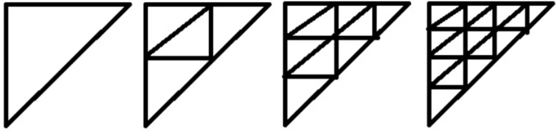
Now we examine whether the analytic results can be veried numerically. As we can see in Figure 3, for parameters (D_P, D_R, D_T) = (0.1,0.3,0.01) the system is unstable as the population of the trees dies out where people rst start to harvest. Note that in the case of T = 0 the derivatives in the rst two equations will become innitely large, resulting in the loss of validity of our model. To avoid such problems we will only consider the case of suciently large values of T and say that for values near zero the populations will die out.

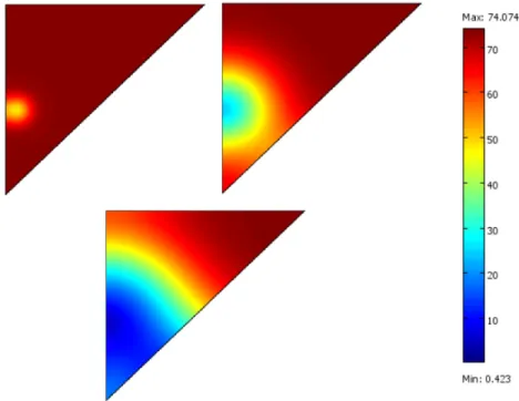
However, as we increase the value of D_T, system (6) becomes stable e.g. for values (D_P, D_R, D_T) = (0.1,0.3,1)as the solution converges to the coexistence equilibrium (7) (see Figure 4). Note that in this case the sucient condition in Theorem 3 does not hold, but Theorem 4 does hold, i.e. the system may become unstable for certain D_T values but will become stable for suciently large ones.

Fig. 3. The unstable case - the number of trees at times t = 1 (upper left), t = 57 (upper right) and t= 105 (bottom) for constants (D_P, D_R, D_T) = (0.1,0.3,0.01). The trees die out at timet = 106 at the rst human settlement

Fig. 4. The stable case - the number of trees at times t = 6 (upper left), t = 120 (upper right) and t = 476 (right) for constants (DP, DR, DT) = (0.1,0.3,1). Although the number of the trees decreases as time goes by, they do not die out, but rather have a constant positive density on the island, which corresponds to the value which can be computed from (7)

4 Conclusions

In this paper we extended the original models of [12, 13] into a system of partial dierential equations. We examined the properties described before involving the stabilizing eect of tree diusion. It turned out that these are more or less similar to the ones of the one- dimensional case, i.e. the increase of the diusion of the trees stabilizes the system. We also conducted some numerical experiments, which also conrm our theorems.

References

[1] Anagnost, J.J., Desoer, C.A. Circuits systems and signal process (1991) 10: 101.

https://doi.org/10.1007/BF01183243

[2] Bahn, P.G., Flenley, J., Easter Island, Earth Island. Thames and Hudson, New York (1992)

[3] Basener, W., Brooks, B., Radin, M., Wiandt, T., Rat instigated human population collapse on Easter Island. Nonlinear Dynamics, Psychology, and Life Sciences, Vol. 12, No. 3, 227240 (2008)

[4] Basener, W., Brooks, B., Radin, M., Wiandt, T., Spatial eects and Turing instabilities in the invasive species model. Nonlinear Dynamics, Psychology, and Life Sciences, Vol.

15, No. 4, 455464 (2011)

[5] Casten, R. G., Holland, C. J., Stability properties of solutions to systems of reaction- diusion equations. SIAM J. Appl. Math, Vol. 33, No. 2 (1977)

[6] Courant, R., Hilbert, D., Methoden der mathematischen Physik I. Springer (1931) En- glish transl.: Methods of Mathematical Physics, Vol. I., Interscience (1953)

[7] Hunt, T., Rethinking the fall of Easter Island: New ecidence points to an alternative explanation for a civilization's collapse. American Scientist, Vol. 94, 412419 (2006) [8] Hunt, T., Rethinking Easter Island's ecological catastrophe. Journal of Archaeological

Science, Vol. 34, 485502 (2007)

[9] Hurwitz, A., On the conditions under which an equation has only roots with negative real parts. Math. Ann., Vol. 46, 273284 (1895) Also in: Selected Papers on Mathemat- ical Trends in Control Theory, Dover, New York, 7082 (1964)

[10] Othmer, H. G., Scriven L. E., Interactions of reaction and diusion in open systems.

Ind. Eng. Chem. Fundamen., Vol. 8, No. 2, 302313 (1969)

[11] Routh, E. J., A Treatise on The Stability of Motion. London, U.K., Macmillan (1877) [12] Takács, B., Horváth, R., Faragó, I., The eect of tree-diusion in a mathematical model

of Easter Island's population. Electron J Qual. Theory Dier. Equ., No. 84, 111. (2016) [13] Takács, B., Analysis of some characteristic parameters in an invasive species model.

Annales. Univ. Sci. Budapest., Sect. Comp., Vol. 45, 119133. (2016)