Internal exact controllability and uniform decay rates for a model of dynamical elasticity equations for

Internal exact controllability and uniform decay rates for a model of dynamical elasticity equations for

incompressible materials with a pressure term

Adriana F. Almeida

, Maria Astudillo

, Marcelo M. Cavalcanti

and Janaina P. Zanchetta

1Federal University of Latin American Integration, 85866-000, Foz do Iguaçu, PR, Brazil

2Department of Mathematics, Federal University of Paraná, 80060-000, Curitiba, PR, Brazil

3Department of Mathematics, State University of Maringá, 87020-900, Maringá, PR, Brazil

Received 14 January 2018, appeared 8 May 2018 Communicated by Vilmos Komornik

Abstract.This paper is concerned with the internal exact controllability of the following model of dynamical elasticity equations for incompressible materials with a pressure term,

φ⁰⁰−∆φ=−∇p,

and it is also devoted to the study of the uniform decay rates of the energy associated with the same model subject to a locally distributed nonlinear damping,

φ⁰⁰−_∆φ+a(x)g(φ⁰) =−∇p,

where Ω is a bounded connected open set of Rⁿ (n ≥ 2) with regular boundaryΓ, φ= (φ₁(x,t), . . . ,φn(x,t)),x = (x1, . . . ,xn)are n-dimensional vectors and p denotes a pressure term. The functiona(x)is assumed to be nonnegative and essentially bounded and, in addition,a(x)≥ a₀> 0 a.e. inω ⊂_{Ω, where}ωsatisfies the geometric control condition. The first result is obtained by applying HUM (Hilbert Uniqueness Method) due to J. L. Lions while the second one is obtained by employing ideas first introduced in the literature by Lasiecka and Tataru.

Keywords: internal exact controllability, incompressible materials, non linear damping, uniform decay rates.

2010 Mathematics Subject Classification: 35B40, 35B35, 35L99, 93D220.

1 Introduction

1.1 Description of the problem.

Let Ω be a bounded connected open set of Rⁿ (n ≥ 2) with regular boundary Γ. Let Q = Ω×]0,T[be a cylinder whose lateral boundary is given byΣ=_Γ×]0,T[.

BCorresponding author. Email: mastudillo86@gmail.com

Consider the following problem















φ⁰⁰−_∆φ=−∇p inQ, divφ=0 inQ,

φ=ψ on Σ,

φ(0) =φ⁰, φ⁰(0) =φ¹ inΩ.

(1.1)

System (1.1) was studied by J. L. Lions [26], motivated by dynamical elasticity equations for incompressible materials. Assuming that Ω is strictly star-sharped with respect to the origin, that is, there existsγ>0 such that

m·ν≥ γ>0 on Γ, (1.2)

(wherem(x) =x = (x₁, . . . ,x_n)_andνis the exterior unitary normal) J.L. Lions [26] proved that the normal derivative of the solutionφof the (1.1) belongs to(L²(_Σ))ⁿwhile A. R. Santos [35]

established the boundary exact controllability for problem (1.1). In this direction it is worth mentioning the work due to Cavalcanti et al. [10], in which boundary exact controllability of the viscoelastic equation

φ⁰⁰−_∆φ−

Z _t

0 g(t−s)_∆φ(s)ds=−∇p, has been studied.

System (1.1) may be obtained from Newton’s second law considering small deflections of Ω, where Ω is a solid body composed of elastic, isotropic, incompressible materials (like some rubber types). For more information on the physical interpretation of this model see A. R. Santos [34] and Cavalcanti et al. [10].

Inspired by the above mentioned works we study, in natural way, in Section 2, the internal exact controllability of the system















φ⁰⁰−_∆φ= −∇p+hχω inQ, divφ=0 inQ,

φ=0 onΣ,

φ(0) =φ⁰, φ⁰(0) =φ¹ inΩ,

(1.3)

where∆φ= (_∆φ₁, . . . ,∆φ_n)_,φ⁰⁰= (φ₁⁰⁰, . . . ,φ⁰⁰_n)_{, div}φ=_∑ⁿ_i=1 ^∂φ_∂xⁱ

i and p= p(x,t)is the pressure term. In addition,ω ⊂ _Ωandχω is the characteristic function ofω whereω is a neighbour- hood of the boundaryΓsatisfying the well-known geometric control conditions.

The exact controllability problem for system (1.3) is formulated as follows: given T > ₀ large enough, for every initial date{φ⁰,φ¹}in a suitable space, it is possible to find a control hsuch that the solution of (1.3) satisfies

φ(x,T) =φ⁰(x,T) =0.

Next, in Section 3, we are going to investigate the uniform decay rates of the energy associated with problem (1.1) subject to a locally distributed nonlinear damping as follows















φ⁰⁰−_∆φ+a(x)g(φ⁰) =−∇p in Ω×(0,∞), divφ=0 inΩ×(0,∞),

φ=_{0 onΣ,}

φ(0) =φ⁰, φ⁰(0) =φ¹ inΩ,

(1.4)

where a∈ L^∞(_Ω)is a nonnegative function such that

a(x)≥a₀>0 inω ⊂_Ω (1.5)

and

g :Rⁿ−→_Rⁿ

s7−→g(s) = [g_i(s_i)]_i=1,...,n ^(1.6) where, for all i=1, . . . ,n, g_i :R−→_Ris a function such that











g_i is continuous monotonic increasing and g_i(0) =0, g_i(s_i)s_i >0 ∀ s_i 6=0,

k|s_i|² ≤ g_i(s_i)s_i ≤K|s_i|² ∀ |s_i| ≥1, for some positive constantsk and K.

(1.7)

1.2 Main goal, methodology and previous results.

The main goal of this paper is twofold: First, to obtain the exact internal controllability of the system (1.3) and then use this result to prove that the solutions of problem (1.4) decay exponentially to zero.

System (1.1) was first introduced by J. L. Lions [26]. In his work, J. L. Lions proved the hidden regularity property holds for this linear system, under the condition that the domain is star-shaped. Taking advantage of this property and an inverse inequality due to Cavalcanti et al. [10], we are able to obtain the direct and inverse inequalities needed to obtain the internal controllability.

In order to obtain the stabilization result, we use an approach first introduced by Lasiecka and Tataru in [20] which allows us not to impose any growth condition of the function gnear the origin and show that the energy decays as fast as the solution of an associated differential equation. Indeed, we are able to establish general decay rates of the energy given by

E(t)≤S t

T₀ −1

, ∀t>T₀ and driven by the solution S(t)of the nonlinear ODE

St+q(S(t)) =0,

whereqis a strictly increasing function in connection with the damping termg(u_t). Moreover, under some extra conditions on the class of nonlinear dissipation and assuming that the pressure is constant, we give examples of the explicit decay rates.

A different but related approach is provided by Alabau-Boussouira and Ammari in [3], where the authors obtained sharp, simple and quasi-optimal decay rates for nonlinearly damped abstract infinite-dimensional systems. The method employed by the authors relies on an observability inequality for the conservative system and some comparison properties, com- bining optimal geometric conditions as provided by Bardos et al. [6] with an optimal-weight convexity method of Alabau-Boussouira (see [1] and [2]).

On the other hand, although the bibliography concerning the wave equation subject to a locally distributed damping is truly long, see, for instance, [1,2,6,12–18,21,22,27–29,31,38,40], and a long list of references therein, it seems that there exist just few papers in connection

with control or stabilization for the model of dynamical elasticity equations for incompress- ible materials introduced by J. L. Lions [26]. In [33] Oliveira and Charão also studied the decay properties of the solutions of an incompressible vector wave equation with a locally distributed nonlinear damping. However, in order to obtain the algebraic decay rate to zero of the solution, the authors imposed some extra technical conditions on the function g like the fact that the partial derivative of gis positive definite which will not be necessary in our present study. In order to get this result, the authors used multiplier methods and a lemma due to Nakao. The exponential decay rate of the energy for the case of an incompressible vector wave equation with localized linear dissipation was obtained by Araruna et al. [4]. In a more general framework, a problem that is similar to (1.1), is studied in [19], where Ammari, Feireisl and Nicaise proved exponential and polynomial decay rates for an acoustic system with spatially distributed damping.

2 Internal exact controllability

In what follows, we consider the Hilbert spaces

V ={v∈ (H₀¹(_Ω))ⁿ and divv =0 in Ω}, (2.1) and

H={v∈ (L²(_Ω))ⁿ, divv=0 and v·ν=0 on Γ}, (2.2) equipped with their respective inner products

((u,v)) =

∑

((u_i,v_i))_H1

0(_Ω), (2.3)

(u,v) =

∑

(u_i,v_i)_L2(_Ω). (2.4) We also consider

V = {ϕ∈(D(_Ω))ⁿ_{, div}ϕ=₀}_{, (2.5)} and

W =V∩(H²(_Ω))ⁿ. (2.6)

We have thatV is dense inV with topology induced byVand

H=V^(L2(Ω))n. (2.7)

We observe that throughout this paper repeated indexes indicate summation from 1 ton.

2.1 Direct and inverse inequalities Let us consider the following problem















φ⁰⁰−_∆φ=−∇p inQ, divφ=0 inQ,

φ=_{0 onΣ,}

φ(0) =φ⁰, φ⁰(0) =φ¹ inΩ.

(2.8)

Firstly, observe that following the arguments [37] we can show that for regular initial data the problem (2.8) is equivalent to the problem

(

φ⁰⁰+Aφ=0 inQ,

φ(0) =φ⁰, φ⁰(0) =φ¹ inΩ, (2.9) where A is Stokes operator defined as follows: A : (H²(_Ω))ⁿ∩V → H given by Au := P(−_∆u) _where P _: (L²(_Ω))ⁿ → H is the orthogonal projector in (L²(_Ω))ⁿ _onto H and ∆ : (H²(_Ω))ⁿ∩V →(L²(_Ω))ⁿ is the Laplace operator with Dirichlet boundary conditions.

In this section we are going to obtain the direct and inverse inequalities to problem (2.8) which is enough to apply HUM (Hilbert Uniqueness Method) in order to obtain the above mentioned exact controllability. For this end we will employ the multiplier technique. The main results of this section are Theorem 2.1and Theorem2.4below.

Theorem 2.1. Let{φ⁰,φ¹} ∈ H×V⁰ andφthe ultra weak solution of the problem(2.8). Then, there exists a constant C₁>0such that

Z _T

0

Z

ω

|φ|²dxdt≤C₁

|φ⁰|²_H+kφ¹k²_V0

. (2.10)

Proof. Sinceφ is the ultra weak solution to problem (2.8) then making use of standard prop- erties of ultra weak solutions for linear problems (see Cavalcanti [10, Section 5] or Lions [25, Chap. 1, Section 4]) there existsC₀>0 such that

kφk²_L∞(0,T;H)+kφ⁰k²_L∞(0,T;V0)≤ C0

|φ⁰|²_H+kφ¹k²_V0

. (2.11)

From (2.11) and L^∞(0,T;H),→ L²(0,T;H)we have the desired result.

Remark 2.2. Arguing as in [7, Chap. 5] or [39, Chap. 2] it is possible to show the existence of a function p ∈ H⁻¹(0,T;L²₀(_Ω))such that (1.3) is satisfied inD⁰(Q). Moreover, there exists C>0 such that

kpk_H−1(0,T;L²₀(_Ω))≤ C(|φ¹|_H+kφ⁰k_V+khχ_ωk_L2(0,T;H)), (2.12) where L²₀(_Ω)≈ L²(_Ω)/R.

Remark 2.3. As it is stated in Lions [25, Chap. I, Lemma 3.7] ifφ∈ (H₀¹(_Ω)∩H²(_Ω))ⁿ, then

∂φ_i

∂x_k =ν_k∂φ_i

∂ν onΓ; ∀i,k ∈ {1, . . . ,n}. (2.13) Moreover, if divφ=0 inΩ, then as in Lions [25, Chap. II, section 5] we have

∂φ

∂ν·ν=0 on Γ (2.14)

and consequently

ν_i∂φ_i

∂x_k = ν_iν_k∂φ_i

∂ν on Γ. (2.15)

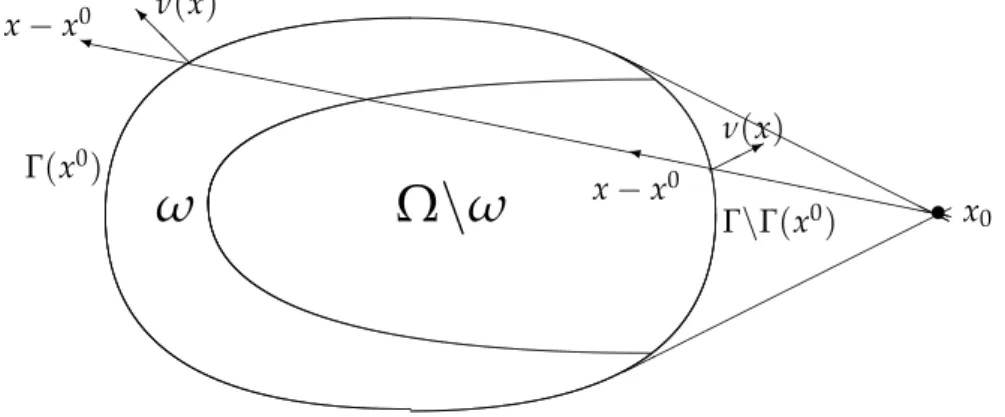
Letx⁰∈ _Rⁿ,m(x) =x−x⁰,x ∈_Rⁿ andR₀=max{km(x)k;x∈_Ω}. We assume thatω⊂_Ωis a neighborhood ofΓ(x⁰)where

Γ0= _Γ(x⁰) ={x∈ _Γ;m(x)·ν(x)>0}, Γ1= _Γ\_Γ(x⁰) ={x∈_Γ;m(x)·ν(x)≤0}, Σ0= _Σ(x₀) =_Γ0(x₀)×[0,T],

Σ1= _Σ\_Σ0 =_Γ1(x0)×[0,T].

(2.16)

As an example of a domain Ω satisfying the above assumption let us consider the Fig- ure2.1 below:

Γ(x⁰)

Γ\_Γ(x⁰)

ω Ω \ _ω

H HH HH HH

H H

``

``

``

``

``

``

``

``

``

``

``

``

``

`` i

y x−x⁰

* ν(x)

@

@ x−x⁰ Iν(x)

``•

Figure 2.1: Description of a subsetω of a domainΩ which is a neighborhood ofΓ(x⁰).

Theorem 2.4. Let us consider T > T₀, where T₀ = 2R₀, as in Theorem 3.3 due to Cavalcanti et al. [10]. Then, there exists a constant C₂>0such that

|φ⁰|²_H+kφ¹k²_V0 ≤C2

Z _T

0

Z

ω

|φ|²dxdt. (2.17)

Proof. Suppose that the following estimate holds kθ⁰k²_V+|θ¹|²_H ≤C₂

Z _T

0

Z

ω

|θ⁰|²dxdt, (2.18)

whereθ is solution of the problem (2.8) with initial data {θ⁰,θ¹} ∈V×H. Then we have the desired result. Indeed, take{φ⁰,φ¹} ∈H×V⁰. Since−φ¹ ∈V⁰and the operator−_∆:V−→V⁰ is an isometric isomorphism, there existsη∈V such that

−_∆η= −φ¹. (2.19)

Let us define

ψ(t) =

Z _t

0 φ(s)ds+η, (2.20)

whereηsatisfies (2.19) andφis the solution to problem















φ⁰⁰−_∆φ=−∇(_∂t^∂p) inQ, divφ=0 inQ,

φ=_{0 onΣ,}

φ(0) =φ⁰, φ⁰(0) =φ¹ inΩ.

(2.21)

Thus we have thatψis the solution to problem















ψ⁰⁰−_∆ψ=−∇p in Q, divψ=0 inQ,

ψ=0 onΣ,

ψ(0) =η, ψ⁰(0) =φ⁰ inΩ.

(2.22)

From (2.18) and (2.22) we have

|φ⁰|²_H+kφ¹k²_V0 ≤C₂ Z _T

0

Z

ω

|φ|²dxdt.

We will prove (2.18) in several steps.

By Theorem 3.3 due to Cavalcanti et al. [10], for T > T₀ = 2R₀ the following inequality holds

E_θ(0)≤C Z _T

0

Z

Γ0

∂θ

∂ν

2

dΓdt, (2.23)

whereθ is the weak solution of the problem (2.8) with the initial data{θ⁰,θ¹} ∈V×H.

Lemma 2.5. Let m∈(C¹(_Ω))ⁿ.Then, for all regular solutions of (2.8), the following identity holds h∇p,m· ∇φi_L2(Q)ⁿ =h∇p,φ· ∇mi_L2(Q)ⁿ− h∇p,φ(divm)i_L2(Q)ⁿ.

Proof. Let us consider

X= −

Z _T

0

Z

Ω

∂p

∂x_im_k∂φ_i

∂x_kdxdt.

Integrating by parts with respect tox_k and using the fact thatφ=0 onΣ, we get X=

Z _T

0

Z

Ω

∂

∂x_k ∂p

∂x_i ·m_k

·φ_idxdt

=

Z _T

0

Z

Ω

∂²p

∂x_i∂x_km_kφ_idxdt+

Z _T

0

Z

Ω

∂p

∂x_i

∂m_k

∂x_kφ_idxdt.

(2.24)

Integrating by parts the first integral, with respect tox_i, we obtain Z _T

0

Z

Ω

∂²p

∂x_i∂x_km_kφ_idxdt= −

Z _T

0

Z

Ω

∂p

∂x_k

∂m_k

∂x_i φ_idxdt−

Z _T

0

Z

Ω

∂p

∂x_km_k∂φ_i

∂x_idxdt.

Since divφ=0 on Q, we conclude that Z _T

0

Z

Ω

∂²p

∂x_i∂x_km_kφ_idxdt= −

Z _T

0

Z

Ω

∂p

∂x_k

∂m_k

∂x_i φ_idxdt.

Therefore,

X=−

Z _T

0

Z

Ω

∂p

∂x_k

∂m_k

∂x_i φ_idxdt+

Z _T

0

Z

Ω

∂p

∂x_i

∂m_k

∂x_kφ_idxdt and the proof is finished.

Lemma 2.6. Let T > T0 andε> 0be such that T−2ε > T0. Letθ be the solution of problem(2.8) with initial data{θ⁰,θ¹} ∈V×H. Then, there exists C>0such that

E_θ(0)≤C Z _T−ε

ε

Z

Γ0

∂θ

∂ν

2

dΓdt. (2.25)

Proof. Sinceθis the weak solution of problem (2.8),θ∈ C([0,T],V)∩C¹([0,T],H)∩C²([0,T],V⁰). In particular,















θ⁰⁰−_∆θ= −∇p inC([0,T−2ε],V⁰), divθ=0 inΩ×(0,T−2ε),

θ =0 onΓ×(0,T−2ε), θ(0) =θ⁰, θ⁰(0) =θ¹ inΩ.

(2.26)

From (2.23) and (2.26) we have

E_θ(0)≤C Z _T−2ε

0

Z

Γ0

∂θ

∂ν

2

dΓdt. (2.27)

Let 0≤t≤ T−2εand defineη(t) =θ(t+ε)and∇q=∇p(x,t+ε). Then,















η⁰⁰−_∆η= −∇q inC([_0,T−2ε]_,V⁰)_, divη=0 inΩ×(0,T−2ε),

η=0 onΓ×(0,T−2ε),

η(0) =θ(ε), η⁰(0) =θ⁰(ε) in Ω,

(2.28)

analogously to what we have done in (2.27), we obtain, E_η(0)≤C

Z _T−2ε

0

Z

Γ0

∂η

∂ν

2

dΓdt. (2.29)

SinceE_η(0) =E_θ(ε) =E_θ(0)and making the change of variables=t+ε, we infer E_θ(0)≤C

Z _T−ε

ε

Z

Γ0

∂θ

∂ν

2

dΓdt.

FixT >T₀ andε >0 such thatT−2ε> T₀. Let us considerh∈(C¹(_Ω))ⁿ such that











h·ν ≥0 for everyx ∈_Γ, h= νonΓ0,

h= 0 inΩ\ω.

Letη∈C¹(0,T)such thatη(0) =η(T) =0 and η(t) =1 in]ε,T−ε[. Let us definer(x,t) =η(t)h(x)which belongs[W^1,∞(Q)]ⁿand satisfies















r(x,t) =ν(x), for every(x,t)∈ _Γ0×]ε,T−ε[, r(x,t)·ν(x)≥0, for every(x,t)∈_Γ×]0,T[, r(x, 0) =r(x,T) =0, for every x∈_Ω, r(x,t) =0, for every(x,t)∈(_Ω\ω)×]0,T[.

(2.30)

Lemma 2.7. Let T > T₀ andε > 0 be such that T−2ε > T₀. Letθ be the solution of problem(2.8) with initial data{θ⁰,θ¹} ∈V×H.Then, there exists C >0such that

E_θ(0)≤C Z _T−ε

ε

Z

ω

|θ|²+|θ⁰|²+|∇θ|²dxdt, (2.31)

where∇θ means









∂θ1

∂x1 · · · _∂x^∂θn .. 1

. . .. ...

∂θ1

∂xn · · · _∂x^∂θn

1









. (2.32)

Proof. Initially considering the regular initial data, one obtains the general result using density arguments. In equation (2.8)₁, taking the inner product in (L²(_Ω))ⁿ of θ⁰⁰−_∆θ+∇p and r· ∇θ, and integrating in [0,T], we obtain

1 2

Z _T

0

Z

γ

r·ν

∂θ

∂ν

2

dγdt= ¹ 2

Z _T

0

Z

Ω(divr)(|θ⁰|²− |∇θ|²)dxdt+

Z _T

0

Z

Ω

∂θ_i

∂x_j

∂r_k

∂x_j

∂θ_i

∂x_kdxdt

−

Z _T

0

Z

Ωθ_i⁰r⁰_k∂θ_i

∂x_kdxdt+

Z _T

0

Z

Ω

∂p

∂x_ir_k∂θ_i

∂x_kdxdt.

(2.33)

Indeed, note that Z _T

0

(θ⁰⁰,r· ∇θ)dt−

Z _T

0

(_∆θ,r· ∇θ)dt=−

Z _T

0

(∇p,r· ∇θ)dt. (2.34) Introduce the notations

J₁ :=

Z _T

0

(θ⁰⁰,r· ∇θ)dt, J₂ :=−

Z _T

0

(_∆θ,r· ∇θ)dt, J₃ :=−

Z _T

0

(∇p,r· ∇θ)dt.

Next, we are going to estimate these terms.

Using integration by parts and the properties of the function r(x,t) defined in (2.30), we deduce J₁, satisfies

J₁=

Z _T

0

(θ⁰⁰,r· ∇θ)dt=−

Z _T

0

Z

Ωθ⁰_ir⁰_k∂θ_i

∂x_kdxdt−

Z _T

0

Z

Ωθ⁰_ir_k∂θ⁰_i

∂x_kdxdt

| {z }

Je1

.

Then Gauss’s Formula yields Z

Ω

∂

∂x_k

θ

02 i r_k

dx=

Z

Γθ

02 i r_kν_kdΓ, and sinceθ⁰_i(x,t) =0 onΣ, we deduce that

Je₁ =−¹ 2

Z _T

0

Z

Ωθ

02 i

∂r_k

∂x_kdxdt.

Thus

J₁ = −

Z _T

0

Z

Ωr⁰_k∂θ_i

∂x_kθ⁰_idxdt+¹ 2

Z _T

0

Z

Ωθ

02 i

∂r_k

∂x_kdxdt

= −

Z _T

0

(θ⁰,r⁰· ∇θ)dt+ ¹ 2

Z _T

0

Z

Ω|θ⁰|²divr dxdt.

(2.35)

Furthermore, we have for the term J₂ J₂ :=−

Z _T

0

(_∆θ,r· ∇θ)dt=−

Z _T

0

Z

Ω

∂²θ_i

∂x²_j r_k∂θ_i

∂x_kdxdt.

From Gauss’s formula and (2.13), we have J₂=

Z _T

0

Z

Ω

∂θ_i

∂x_j

∂

∂x_j

r_k∂θ_i

∂x_k

dxdt

| {z }

Je2

−

Z _T

0

Z

Γr_k∂θ_i

∂x_k

∂θ_i

∂νdΓdt. (2.36)

Notice that

Je₂ =

Z _T

0

Z

Ω

∂θ_i

∂x_j

∂r_k

∂x_j

∂θ_i

x_k dxdt+ ¹ 2

Z _T

0

Z

Ωr_k ∂

∂x_k ∂θ_i

∂x_j 2

dxdt

| {z }

ee J₂

. (2.37)

From Gauss’s formula and (2.13), we deduce that ee

J₂ = ¹ 2

Z _T

0

Z

Γr_kν_k ∂θ_i

∂ν 2

dΓdt−¹ 2

Z _T

0

Z

Ω

∂r_k

∂x_k ∂θ_i

∂x_j 2

dxdt. (2.38)

Thus from (2.36), (2.37), (2.38) and (2.13), we have

J2=

Z _T

0

Z

Ω

∂θ_i

∂x_j

∂r_k

∂x_j

∂θ_i

x_k dxdt− ¹ 2

Z _T

0

Z

Ωdivr(|∇θ|²)dxdt− ¹ 2

Z _T

0

Z

Γ(r·ν)

∂θ

∂ν

2

dΓdt. (2.39) For the term J₃ we have

J₃= −

Z _T

0

(∇p,r· ∇θ)dt=−

Z _T

0

Z

Ω

∂p

∂x_ir_k∂θ_i

∂x_kdxdt. (2.40)

Therefore, from (2.34), (2.35), (2.39) and (2.40) we infer 1

2 Z _T

0

Z

Γ(r·ν)

∂θ

∂ν

2

dΓdt= ¹ 2

Z _T

0

Z

Ω(divr)(|θ⁰|²− |∇θ|²)dxdt−

Z _T

0

(θ⁰,r⁰· ∇θ)dt +

Z _T

0

Z

Ω

∂θ_i

∂x_j

∂r_k

∂x_j

∂θ_i

∂x_kdxdt+

Z _T

0

Z

Ω

∂p

∂x_ir_k∂θ_i

∂x_kdxdt.

(2.41)

Note that by Lemma2.5we have that Z _T

0

Z

Ω

∂p

∂x_ir_k∂θ_i

∂x_kdxdt=h∇p,−θ· ∇r+θ(divr)i_H−1(Q)ⁿ,H₀¹(Q)ⁿ. (2.42) Therefore

Z _T

0

Z

Ω

∂p

∂x_ir_k∂θ_i

∂x_kdxdt

≤δk∇pk²_H−1(Q)ⁿ+C_δ Z _T

0

Z

ω

|θ|²+|θ⁰|²+|∇θ|²dxdt.

Using the properties of r(x,t) and estimating others term on the right side of equality (2.41), we obtain that

1 2

Z _T

0

Z

Γ(r·ν)

∂θ

∂ν

2

dΓdt≤δk∇pk²_H−1(Q)ⁿ+C Z _T

0

Z

ω

|θ|²+|θ⁰|²+|∇θ|²dxdt. (2.43)

Therefore, by Lemma2.6and (2.43) we have E_θ(0)≤ ¹

2 Z _T−ε

ε

Z

Γ0

∂θ

∂ν

2

dΓdt= ¹ 2

Z _T−ε

ε

Z

Γ0

(r·ν)

∂θ

∂ν

2

dΓdt

≤ ¹ 2

Z _T

0

Z

Γ(r·ν)

∂θ

∂ν

2

dΓdt

≤ δk∇pk²_H−1(Q)ⁿ+C Z _T

0

Z

ω

|θ|²+|θ⁰|²+|∇θ|²dxdt.

(2.44)

Using the factk∇pk²

H⁻¹(Q)ⁿ ≤ CE_θ(0), by (2.44) and choosingδsmall enough we have E_θ(0)≤C

Z _T

0

Z

ω

|θ|²+|θ⁰|²+|∇θ|²dxdt.

Since the inequality above is valid for allT> T₀, in particular forT−2ε, proceeding as in the demonstration of Lemma 2.6we have the desired result.

Remark 2.8. According to the proof of Lemma 2.3 in J. L. Lions [25] we can construct a neighbourhood ˆω ofΓ0 such thatΩ∩ωˆ ⊂ωand we can to build a vector field ˆr for ˆw. Then, we get analogously, that

E_θ(0)≤ C Z _T−ε

ε

Z

ˆ ω

|θ|²+|θ⁰|²+|∇θ|²dxdt.

Now, let us consider a functionr=r(x,t)∈W^1,∞(Q)that satisfies























r(x,t)≥0, for every (x,t)∈_Ω×]0,T[, r(x,t) =1, for every (x,t)∈ωˆ×]ε,T−ε[_, r(x,t) =0, for every (x,t)∈(_Ω\ω)×]0,T[,

0<r(x,t)<1, for every (x,t)∈ (ω\ωˆ)×]0,T[and ˆω×(]0,ε]∪[T−ε,T[), r(x, 0) =r(x,T) =0, for every x∈ _Ω,

|∇r|²

r ∈ L^∞(ω×]0,T[ ).

(2.45)

The function r can be chosen as follows r(x,t) = ρ²(x)η(t) where η ∈ C¹(0,T) and it

satisfies 









η(0) =η(T) =0, η(t) =1, in ]ε,T−ε[,

0<η(t)<_{1, in} ]_0,ε[ ∪ ]T−_ε,T[_, andρ∈C¹(_Ω)satisfies











ρ(x) =1, for every x∈ ω,ˆ ρ(x) =0, for every x∈ _Ω\ω, 0<ρ(x)<1, for every x∈ω\ω.ˆ

Proposition 2.9. Let us consider T > T₀ and ε > 0 such that T−2ε > T₀ andθ the solution of problem(2.8)with initial data {θ⁰,θ¹} ∈V×H.Then, there exists a constant C >0such that

E_θ(0)≤C Z _T

0

Z

ω

|θ|²+|θ⁰|²dxdt. (2.46)

Proof. Initially we consider regular initial data and one obtains the general result using density arguments. In equation (2.8)₁, taking the inner product in (L²(_Ω))ⁿ of θ⁰⁰−_∆θ+∇p andrθ and integrating in[0,T], we obtain

Z _T

0

Z

Ωθ⁰⁰_irθ_idxdt−

Z _T

0

Z

Ω∆θirθ_idxdt=−

Z _T

0

Z

Ω

∂p

∂x_irθ_idxdt. (2.47) Next, we are going to estimate the terms in (2.47).

Denote by

I₁ :=

Z _T

0

Z

Ωθ⁰⁰_irθ_idxdt.

I₂ :=−

Z _T

0

Z

Ω∆θirθ_idxdt, I₃ :=−

Z _T

0

Z

Ω

∂p

∂x_irθ_idxdt.

Using the properties of the functionr(x,t)defined in (2.45) and making use of the equality (θ_i⁰,rθ_i)⁰ = (θ⁰⁰_i ,rθ_i) + (θ_i⁰,r⁰θ_i) + (θ⁰_i,rθ_i⁰), we have that I₁ can be estimated as follows

I₁ =

Z _T

0

Z

Ωθ⁰⁰_irθ_idxdt=−

Z _T

0

Z

Ωθ_i⁰r⁰θ_idxdt−

Z _T

0

Z

Ωθ⁰_irθ_i⁰dxdt. (2.48) Notice that using Gauss’s formula and taking θ = 0 on Σ into account, we infer that I2

verifies

I₂ =−

Z _T

0

Z

Ω∆θ_irθ_idxdt=

Z _T

0

Z

Ω∇θ_i(∇r)θ_i+r|∇θ_i|²dxdt. (2.49) Replacing (2.48), (2.49) in (2.47), we obtain

Z _T

0

Z

Ωr|∇θ_i|²dxdt=

Z _T

0

Z

Ωr|θ_i⁰|²dxdt+

Z _T

0

Z

Ωr⁰θ⁰_iθ_idxdt

−

Z _T

0

Z

Ω∇θ_i(∇r)θ_idxdt−

Z _T

0

Z

Ω

∂p

∂x_irθ_idxdt.

(2.50)

By Young’s inequality we obtain that Z _T

0

Z

Ωr⁰θ_i⁰θ_idxdt≤C Z _T

0

Z

Ω(|θ_i⁰|²+|θ_i|²)dxdt. (2.51) Making use of the inequalityab ≤ ¹₂a²+ ¹₂b², we can write

Z _T

0

Z

Ω∇θ_i(∇r)θ_idxdt

=

Z _T

0

Z

Ωr¹²∇θ_i∇r r¹² θ_idxdt

≤ ¹ 2

Z _T

0

Z

Ωr|∇θ_i|²+¹ 2

Z _T

0

Z

Ω

|∇r|²

r |θ_i|²dxdt.

(2.52)

By the Cauchy–Schwarz inequality and by Young’s inequality we have that Z _T

0

Z

Ω

∂p

∂x_irθ_idxdt≤δkpk²_H−1(0,T;L²(_Ω)ⁿ)+C_δkrθk_H1

0(0,T;L²(_Ω)ⁿ) (2.53) for anyδ>_0.

Combining (2.51), (2.52) and (2.53) we obtain Z _T

0

Z

ω

r|∇θ|²dxdt≤ C Z _T

0

Z

ω

|θ⁰|²+|θ|²dxdt+δkpk²_H−1(0,T;L²(_Ω)ⁿ). (2.54) However,

Z _T−ε

ε

Z

ˆ ω

|∇θ_i|²dxdt=

Z _T−ε

ε

Z

ˆ ω

r|∇θ_i|²dxdt≤

Z _T

0

Z

ω

r|∇θ_i|²dxdt. (2.55) From (2.54) and2.55, we obtain

Z _T−ε ε

Z

ˆ ω

|∇θ_i|²dxdt≤ C Z _T

0

Z

ω

|θ⁰_i|²+|θ_i|²dxdt+δkpk²_H−1(0,T;L²(_Ω)ⁿ). (2.56) From Remark2.8and (2.56) we obtain

E_θ(0)≤C Z _T

0

Z

ω

|θ⁰|²+|θ|²dxdt+δkpk²_H−1(0,T;L²(_Ω)ⁿ). (2.57) By (2.57) and choosingδ small enough we have

Eθ(0)≤C Z _T

0

Z

ω

|θ⁰|²+|θ|²dxdt. (2.58)

Proposition 2.10. Let T >T₀andε>0be such that T−2ε>T₀,ωa neighborhood ofΓ0previously cited andθ the solution of the(2.8) with{θ⁰,θ¹} ∈ V×H.Then, there exists a constant C>0such that

Z _T

0

Z

ω

|θ|²dxdt≤C Z _T

0

Z

ω

|θ⁰|²dxdt. (2.59)

Proof. We argue by contradiction. Let us suppose that (2.59) is not verified, then for every m∈ _Nlet{θ⁰_m,θ_m¹} ∈V×Hbe a sequence of initial data where the corresponding solutions {θ_m}of the problem (2.8) verify

mlim→_∞

RT 0

R

ω|θ_m|²dxdt RT

0

R

ω|θ⁰_m|²dxdt

= +_{∞, (2.60)}

or, equivalently,

mlim→_∞

RT 0

R

ω|θ_m⁰ |²dxdt RT

0

R

ω|θ_m|²dxdt =0. (2.61)

Defining

α_m =^qkθ_mk_L2(0,T,Hω) and ψ_m = ^θm

α_m, (2.62)

where Hω ={u; u∈(L²(ω))ⁿ; divu=0 and u·ν=0 on Γ}, then we obtain

kψ_mk_L2(0,T,Hω) =_{1. (2.63)}

It is easy to see that

Eψm = ¹

α²_mE_θm (2.64)

From Proposition2.9 we have E_ψm(₀)≤

Z _T

0

Z

ω

|ψ⁰_m|²+|ψ_m|²dxdt.

then, by (2.61), (2.62) and (2.63)

Eψm(0)≤L. (2.65)

Therefore, there exist subsequences of the{ψ⁰_m},{ψ¹_m}, denoted in the same way, such that ψ_m⁰ *ψ⁰ inV,

ψ_m¹ *ψ¹ inH.

SinceE_ψm(t) =E_ψm(0)≤Lwe conclude that there exist subsequences of{ψ_m}, denoted in the same way, such that

{ψ_m} is bounded in L^∞(0,T;V), (2.66) {ψ⁰_m} is bounded in L^∞(0,T;H). (2.67) From (2.66) and (2.67), we infer that there exist subsequences, denoted in the same way, such that

ψ_m *^∗ ψ (weak star) in L^∞(0,T;V), (2.68) ψ_m⁰ *^∗ ψ⁰ (weak star) in L^∞(0,T;H). (2.69) SinceV,→ His compact, then from Theorem 5.1 due to J. L. Lions [24], we have

ψ_m →ψ in L²(0,T,H). (2.70)

From (2.61) and (2.69) we have that

ψ⁰(x,t) =_{0 in}ω×(_0,T) _(2.71) andψis independent oft inω.

From the above convergence results, we have thatψis solution of problem (2.9) with initial data{ψ⁰,ψ¹} ∈V×H. In order to achieve a contradiction it is enough to prove thatEψ(0) =0.

Indeed, sinceE_ψ(t) =E_ψ(0), we have that|ψ⁰|²_H+kψk²_V =0 henceψ=0 in Qcontradicting (2.63) and (2.70). In order to prove this, we consider the following system

(

ξ⁰⁰+Aξ =0 inQ,

ξ(0) =−ψ¹, ξ⁰(0) = Aψ⁰ inΩ, (2.72) with{−ψ¹,Aψ⁰} ∈H×V⁰, where Ais the Stokes operator.

Taking v(x,t) = ψ⁰(x)−RT

0 ξ(x,s)ds, then v solves (2.9) with initial dates {ψ⁰,ψ¹} ∈ V×H.

Therefore, from the uniqueness of solutions of (2.9) , we have that

v=ψ (2.73)