A comprehensive econometric analysis of the European countries

(1)

Wealthier is healthier? Healthier is wealthier?

A comprehensive econometric analysis of the European countries

REYHAN CAFRI AÇCI

¹

and PINAR KAYA SAMUT

²^p

1Department of International Trade and Management, Faculty of Business and Management Sciences, _Iskenderun Technical University,_Iskenderun, Hatay, Turkey

2Department of Econometrics, Faculty of Economics and Administrative Sciences, Akdeniz University, 07058, Antalya, Turkey

Received: May 2, 2019 • Revised manuscript received: January 23, 2020 • Accepted: March 3, 2020

ABSTRACT

Healthier people contribute more to the development of the economy. Besides, in a better economy, people have a better quality and healthier life. At this stage, one has to ask which one precedes the other: health or wealth? To find the answer, this study aims to investigate the causality relationship between health and inclusive wealth in the European countries for the period of 1990–2015. The causality between health and inclusive wealth scores, which are estimated by cluster and discriminant analyses, is investigated by the panel causality test. The research results indicate bidirectional causality between health and inclusive wealth. A one-way causality is detected in 11 cases as being from inclusive wealth to health and in 8 the other way. Furthermore, a two-way causality is found in 2 countries. Among the results, it is noteworthy that 91% of the countries with causality from inclusive wealth to health are among the healthy countries.

KEYWORDS

inclusive wealth, health, two-step cluster analysis, discriminant analysis, panel causality, the EU JEL CLASSIFICATION INDICES

C33, C38, I15, O52

pCorresponding author. E-mail: pinarsamut@akdeniz.edu.tr

(2)

1. INTRODUCTION

The level of income per capita is an indicator of the average welfare level of people living in a country and the economic power of that country. In this context, human capital is of great importance for income and its distribution. Being one of the basic elements of development, it should be dealt with not only in educational terms but also in health terms, another important dimension that provides a long-lasting technological development and increases total factor productivity (Howitt 2004). In recent years, studies have emphasized that improving people’s health of countries increases the total factor productivity and per capita GDP as a healthy labor force is more productive. Besides, the increase in life expectancy is thought to increase savings and encourage people to receive more education; in turn, more educated people have increased incomes. In addition, it is suggested that being healthy during early childhood and even before birth improves the learning capacity of an individual, providing a more efﬁcient human capital stock in the future (Bloom et al. 2004;Howitt 2004;Fielding–Torres 2009;Kunze 2014). In the words of Mahatma Gandhi, a human rights defender, health is a vital fact that is intertwined with wealth in human life, “It is health that is real wealth and not pieces of gold or silver” (Somoskovi 2013). Moreover, according to the third item titled“good health and well-being”of the United Nations’ Sustainable Development Goals (SDG), it is necessary to be healthy for reducing poverty and ensuring sustainable development (Aghion 2010). Studies on the notion of being healthier as a cause of wealth began to take place and add to the literature (Acemoglu– Johnson 2007;Fielding –Torres 2009;Aghion et al. 2010;Hansen 2012;Kunze 2014).

In the same way that appears to ensure more wealth, the reverse may also be true. It has been suggested that higher-income people are healthier because they have the opportunity to get better nutrition and better-quality healthcare based on the studies investigated the link between the two (Pritchett– Summers 1996; Deaton 2002;Lorentzen et al. 2008; Wilkinson –Pickett 2008;Kozun-Cieslak 2020). However, Deaton (2007)has emphasized the need for both health and wealth at the same time, noting that there are very few things people can do without wealth and that health alone without income is not enough for people to live a good life, either. As far as the authors of the present research have investigated, in the literature, studies that investigate this reciprocal relationship between health and wealth pointed out by Deaton, are rare and limited toMichaud –van Soest (2008)and Adams et al.(2003).

The literature, in general, focuses on whether healthier countries have higher incomes or whether wealthy countries are healthier. Besides, life expectancy and infant mortality are used as health indicators, while wealth is indicated as per capita GDP or as a share of income. In order to determine the effect of wealth on health,Pritchett–Summers (1996)used infant mortality rates and life expectancy as health indicators and per capita GDP as the wealth indicator in their cross-section analyses of the developing countries, Africa and Latin America. Aghion et al.

(2010)investigated whether health can explain the differences in the growth of countries in the framework of internal growth theories for the developed, developing OECD and sub-Saharan African countries. The authors used per capita GDP for growth and life expectancy for the health variable. On the other hand,Acemoglu–Johnson (2007)examined the effects of health on wealth in the poor, middle and rich countries using life expectancy and an instrumental variable, predicted mortality rate, which includes the effects of diseases and global interventions for health variables, GDP and per capita GDP for economic performance variables. Hansen (2012) also used life expectancy for health and GDP per capita for wealth in his study of the

(3)

effect of health on wealth. However, it is emphasized that, where the dynamic panel analysis is performed on 119 countries, the relationship between life expectancy and wealth can be non- monotonic; therefore, the square of life expectancy is also important for the model.Biggs et al.

(2010) used the proportion of tuberculosis in addition to infant mortality rates and life expectancy as health variables in their studies to investigate the effect of wealth upon health in the Latin American countries. For the wealth variable, poverty rate and income inequality are considered together with GDP per capita.

In the studies conducted on a micro basis, the health and wealth indicators have been dealt with more extensively. For instance, Michaud – Van Soest (2008) used the US Health and Retirement Study to investigate the relationship between wealth and health variables for couples aged 51 to 61. In their study, wealth is measured by liquid assets such as individual retirement, bonds-stock, and non-liquid assets such as real estate. Besides, for the health variable: cancer, stroke, blood pressure, diabetes, heart disease, lung disease as well as psychological disorders are taken into consideration.

Our aim is to investigate the causal relationship between health and wealth in the EU, EFTA and EU candidate countries by using more comprehensive health and income indicators between 1990 and 2015. In the literature, life expectancy and mortality rates are generally used as health indicators in the context of macroeconomic perspective. Robine – Ritchie (1991), Pritchett–Summers (1996), Acemoglu– Johnson (2007), Deaton (2007), Pope et al. (2009), Aghion et al. (2010), Biggs et al. (2010), Hansen (2012) are among those, who take life expectancy and/or mortality rates as representatives of health.

In our work,sanitationandtuberculosisrates are also taken into consideration for the health variable, in addition tolife expectancyandchild mortalityrates under the age ofﬁve,“mortality for children under 5” is preferred rather than “death rate”.¹ It has been emphasized in other works that some diseases and deaths originate from lack of clean water and sanitation and, hence, from infectious diseases (Deaton 2002). In addition to sanitation, tuberculosis rates as one of the major infectious diseases are also considered as a health indicator. According to the report published by the World Health Organization (WHO) and the European Center for Disease Prevention and Control (ECDC) in 2019, tuberculosis is still an important public health problem in the EU region (WHO, Regional Ofﬁce for Europe, 2019). Accordingly, the region has 9 out of 30 countries with the highest multidrug-resistant tuberculosis burden in the world. It was emphasized that countries still face various challenges to end tuberculosis in the region. For this reason, this variable was considered important for the health indicator and was included in our analysis.

It is known that there is a strong relationship between clean water, sanitation and health.

Despite the adoption of the EU urban wastewater director in 1991, only 14 of the 28 EU capitals are reported to be fully compliant in 2012, however, it is stated that many countries in Europe lag behind in wastewater treatment, as most of them either do not have tertiary (full) treatment coverage or are low. It is also presented in reports that about 10 million people in the EU and 2.4 billion people worldwide still live without the access to improved sanitation facilities (Andersson 2016; European Comission 2016). Therefore, it was seen that the sanitation variable was important for health indicators within the period covered.

1The death rate variable also includes cases such as work-related accidents, trafﬁc accidents and death from old age.

(4)

The wealth index is often calculated as a composite indicator of the household’s standard of living in studies involving the micro-approach. In the calculation of the index, the assets owned by the household are taken into account. But wealth has often been represented by GDP in the macro-approach studies (Pritchett–Summers 1996;Acemoglu–Johnson 2007;

Hansen 2012). Biggs et al. (2010) included GDP as well as the poverty rate and income inequality in his study. Socio-economic indicators of wealth include education and unemployment (Easton-Brooks –Davis 2007; Markou et al. 2015). Since negative variables were converted to positive for the index, employment was taken into consideration instead of unemployment. The importance given to income inequality in the calculation of the inclusive wealth index draws attention in the studies (UNU-IHDP and UNEP 2014; Roman –Thiry 2016). These studies clearly offer that the growing income inequality should be included in the wealth index to the comparisons of countries. As for the inclusive wealth variables, income inequality, employment rate, and education are taken into account as well as per capita GDP.

As an indicator of the country’s economic power, it is important whether everyone in the society receives a fair share of the country’s income as well as per capita GDP. In addition, the employment rate and the level of higher education are among the indicators of wealth or well- being.

In the first stage of our study, using four health and four inclusive wealth indicators, the health and wealth scores are calculated with the help of the Two-step Cluster and Discrimi- nant analyses. Firstly, the European countries are divided into two clusters as healthy-less healthy and wealthy-less wealthy for each year by Two-step Cluster analysis. These binary variables are, then, taken as dependent variables in the Discriminant analysis, establishing the health and wealth scores of each country for 1990–2015. In the second stage, the existence of causality between these two variables is investigated by the Emirmahmutoglu–Kose (2011) test, where the heterogeneous causality can be examined for each of the countries, as well as for whole panel.

This study consists of five Sections. In addition to the purpose and the importance of the study, the literature on this subject is mentioned in the introduction. The next two Sections introduce the data and method. Section 4 contains theﬁndings, followed by the conclusions in Section 5.

2. DATA

Our health and wealth data sets are concerned with 35 European countries (including 28 EU, 3 EFTA, and 4 EU candidate countries) for the period of 1990–2015.²The sample includes all EU countries, but not all EFTA and EU candidate countries. While Norway, Switzerland and Iceland from the EFTA countries were included in the analysis, Liechtenstein was excluded due to lack of data. In addition, from the EU candidates and potential candidate countries only Turkey, Macedonia, Albania and Bosnia and Herzegovina were analyzed. Serbia and Montenegro were left out due to lack of data prior to 2004.

2Theﬁgures related to many variables are only available for the years between 1990 and 2015, and the missing values for some countries going back 2 or 3 years wereﬁlled in by linear interpolation.

(5)

The variables used in the models as health and inclusive wealth indicators are presented along with their definitions and measurement information in Table 1. The data of the Gini coefﬁcient is taken from the Standardized World Income Inequality Database (Solt 2014), and other data from theWorld Bank Development Indicators(WDI) database.

3. METHODOLOGY

3.1. Cluster and discriminant analyses

In the first stage of the study, a linear discriminant function was estimated to generate health and wealth indices for the European countries. The dependent variable values of this function are obtained by a cluster analysis, which is a multivariate statistical method and an analytical technique that groups the individuals or objects in a meaningful way by taking into account similarities in the basic characteristics (Hair et al. 2010). To determine the similarities between individuals or objects, the distance measures, correlation measures, and similarity measures of quality data are used in the cluster analysis. The homogeneity within the formed clusters as a result of the analysis and the heterogeneity between them are high. The most common distance measures used in the cluster analysis are the distances of Euclid, Minkowski, City-Block (Manhattan) and Mahalanobis. The clustering algorithms can be grouped into two main cat- egories as hierarchical and non-hierarchical. For detailed information, it can be beneﬁtted from the sources ofAnderberg (1973),Everitt (2011), andSarstedt–Mooi (2011).

We use a Two-step Cluster method, which is a hybrid clustering technique consisting of K- means clustering and Ward’s smallest variance technique from the hierarchical methods. Two- step analysis has two main steps as pre-clustering and clustering. In the pre-clustering step, observations are subdivided into smaller sub-clusters using a modiﬁed cluster features tree.

Later, in the clustering stage, each of these sub-clusters is deﬁned as an initial cluster and the Table 1.Model variables

Definition Measurement unit

Health indicators

Mortality Mortality rate, under age 5 Per 1,000 live births

Life expect. Life expectancy at birth Total (years)

Sanitation Improved sanitation facilities % of population with access

Tuberc Incidence of tuberculosis Per 100,000 people

Inclusive wealth indicators

GDP GDP per capita Constant 2010 US$

Gini Income inequality index In net income (%)

Employ Employment to population ratio 15þ, total (%)

Education Mean years of schooling Years

(6)

clusters are combined until optimal clustering is achieved by the agglomerative hierarchical clustering method. The number of clusters can be determined by the researcher as well as by the model. As the distance measure in the Two-step Cluster analysis, log-likelihood which can be calculated for categorical variables as well as continuous variables, or the Euclidean distance measure which requires all continuous variables can be used (Bacher et al. 2004). The Schwarz’s Bayesian information criterion (BIC) or the Akaike Information Criterion (AIC) is used to determine the optimal clusters. The relative contribution of the variables in the clusters is examined by the t-test for continuous variables and the chi-square (c2) test for categorical variables (Rundle-Thiele 2015).

Discriminant analysis is a powerful descriptive and classificatory technique developed by Fisher in 1936. This multivariate statistical method is used to identify the factors that differentiate two or more pre-classiﬁed groups and to predict which group can be assigned upon observation from outside the group (Brown –Wicker 2000). In the discriminant analysis, a discriminant function composed of one dependent and one or more independent variables is estimated. The discriminant function (DF) takes the following form (Hair et al.

2010):

Z_ij¼aþW₁X_1kþW₂X_2kþ. . .þW_nX_nk (1) where

Zjk5discriminant Z score of discriminant functionjfor objectk a5intercept

Wi5discriminant weight for independent variable i Xik5 independent variableifor objectk

In the DF, the dependent variable should be measured on the categorical scale and the independent variables on the metric scale. One DF is estimated for two categorical dependent variables, whereas k-1 DFs are estimated for k grouped multiple discriminant analysis.

The Discriminant analysis calculates the mathematical weights of each discriminator variable. These weights, called ‘discriminant coefﬁcients’, indicate which variable has more discriminability. The discriminant score for each function is calculated by multiplying each case’s independent variable raw score and the coefﬁcient of it. The average discriminant score of the cases belonging to a group represents the centroids of this group (Brown – Wicker 2000).

Discriminant analysis has some important limitations such as multivariate normality, linearity, homogeneity of variance-covariance matrices, the absence of multicollinearity and singularity (Tabachnick–Fidell 2003). The Box’s M test is used to check the multivariate normality, and it is expected to accept the null hypothesis that claims the independent variance is multi-normally distributed. In addition, the validity of the estimated discriminant function should also be examined. If the ratio of between-groups variability to within-group variability is high, this function is assumed as a successful and valid discriminant function. DF is evaluated by Eigenvalue, Canonical Correlation and Wilk’s Lambda values that give these ratios, and by Chi-Square Test which analyses the variability related to group differences (Sharma 1996). Lastly, by determining accuracy hit rates and cross-validation, classiﬁcation accuracy is evaluated. Hit ratio is calculated by dividing the number of correctly classiﬁed observations in each group by the total number of observations.

(7)

3.2. The preliminary tests for the panel causality tests

In the second stage, the causality between health and wealth scores obtained in the first stage for each country for 1990–2015 is investigated by theEmirmahmutoglu–Kose (2011)panel causality test. Before analyzing causality by these tests, cross-section dependency and the heterogeneity of slope coefﬁcients should be investigated with the help of preliminary tests for the causality analysis. Cross-sectional dependence, which means that a shock in one country affects other countries, is investigated by tests that take into account the correlations between units.

In terms of the sample of the study, the test of Cross-Sectional Dependence (CD) ofPesaran (2004)is used which investigates the cross-section dependency in cases where the cross-section dimension (N) is greater than the time dimension (T). This is because, in the otherCD_LMtests developed byBreusch–Pagan (1980)andPesaran (2004), the T > N condition is sought, these tests do notﬁt the sample of the study. As seen in Eq. (2), the CD test is based on the sum of the correlation coefﬁcients (brijÞbetween the cross-sectional residues. The null hypothesis (H₀) of the CD test implies that there is no relationship between the cross sections, and the alternative hypothesis is that there is an association (Pesaran 2004).

CD¼

ffiffiffiffiffiffiffiffiffiffiffiffiffiffiffiffiffiffiffiffi 2T NðN1Þ

s X^N−1

i¼1

X^N

J¼iþ1

brij

!

⇒ N ð0; 1Þ (2) Valid in the cases where the cross-section dimension is greater than the time dimension, Delta tilde (Δ) and Delta tilde adjust~ ðΔ~adjÞhomogeneity tests are developed byPesaran–Yamagata (2008). The tests are calculated as shown in Eq. (3).

~Δ¼ ffiffiffiffi

pN N⁻¹Sk ffiffiffiffiffi

p2k ; ~Δadj¼ ffiffiffiffi

pN N⁻¹SE Z~it

ffiffiffiffiffiffiffiffiffiffiffiffiffiffiffiffiffiffiffi Var

Z~it

r (3)

In the formation, the Swamy test statistic is expressed as S and the number of explanatory variables as k. In Delta tilde adjust statistic, which is a corrected version of the deviation of delta tilde statistic in small samples, the expected and variance values of Z~_it are calculated by the formulations given in Eq. (4).

E Z~it

¼k ; Var Z~it

¼2kðTk1Þ

Tþ1 (4)

In the Delta tests, the alternative hypothesis is expressed in the form of the slope coefficients as being heterogeneous, while the null hypothesis claims the homogeneity of the slope (Pesaran –Yamagata 2008).

The CADF unit root test, one of the second-generation unit root tests used when determining the cross-section dependency, takes into account also heterogeneity. The Cross- Sectionally Augmented Dickey-Fuller (CADF) test developed byPesaran (2007)is the extended version of the ADF regression, calculating by considering the cross-section averages of theﬁrst differences and the lag levels of each country. In the CADF, the time averages calculated for each period are included in the test as a factor causing the cross-section. The basic hypothesis of this test is that each series in the panel is not stationary, and the alternative hypothesis is that at least one unit is stationary (Pesaran 2008).

(8)

3.3. Emirmahmutoglu and Kose (EK) panel causality test

The Emirmahmutoglu and Kose (EK) panel causality test matters in terms of handling the results of causality for each cross-section separately and in terms of providing interpretations on the basis of countries as well. In addition, this test takes into account the cross-sectional dependence and can be used independently of the relationship of cointegration between variables. The heterogeneous mixed panel models are tested with the help of Eq. (5) (Emirmah- mutoglu–Kose 2011).

zi;t¼

m

iþAi1Zi;t−1þ. . .þAikZi;t−kiþ^kⁱ^þdmaxX ⁱ

l¼kiþ1

AilZi;t−1þui;t (5) In the formula, Aikand kiþdmaxi(where kiis the lag structure and dmaxiis the maximal order of integration) represent the parameter matrix and the number of maximum lags of the VAR (Vector Autoregression) model, respectively.

4. EMPIRICAL RESULTS

4.1. Obtaining health and inclusive wealth indices

At this stage, the countries’health and wealth scores for 25 years are obtained using four health and four wealth variables. Firstly, 35 European countries consisting of the EU and EU candidate countries and the EFTA countries, are divided into two clusters as healthy –less healthy and wealthy –less wealthy for each year by the Two-step Cluster analysis. These binary variables attained by the Cluster analysis are taken as dependent variables in the Discriminant analysis, and then the health and wealth scores of each country for 1990–2015 are estimated.

In the Two-step Cluster method, the log-likelihood and the BIC are used as the distance measure and the clustering criterion, respectively, and also the number of clusters is determined as 2 at the beginning of the process. Thus, for the 25-year period, the countries are divided into two groups in terms of health and wealth. By coding the countries as 1 and 2, the dependent variable of the Discriminant analysis is obtained for each year. From the health variables, Mortality and Tuberc, and the wealth variable Gini are taken in the Cluster analysis after being converted to positive contributor variables. The“mortality rate”values are transformed into the

“survival rate”by subtracting from 1,000 and the“incidence of tuberculosis”values are changed to“non-existence of tuberculosis incidents”by subtracting from 100,000. Thus, all the variables are made to be variables that affect health positively. Likewise, Gini index, one of the variables of wealth has been transformed in a way that positively affects the wealth.“Gini income inequality index”(100%) is converted to reﬂect wealth by subtracting from 100.”

The discriminant analysis aims to group individuals with knownpcharacteristics according to these properties. In the discriminant analysis, the dependent variable should be measured on the categorical scale (attained by cluster analysis) and the independent variables on the interval or ratio scale. In this study, health and wealth scores for 1990–2015 are obtained by estimating two DFs for each year. The estimated discriminant functions for health and wealth are seen in Eqs. (6) and (7).

The DF for health indicators:

(9)

D¼b₀þb₁X₁þb₂X₂þb₃X₃þb₄X₄ (6) D¼

1; healthy

2; less healthy orD¼

1; less healthy 2; healthy

X1:mortality; X2:lifeexpect; X3:sanitiation; X4:tuberc The DF for inclusive wealth indicators:

D¼b0þb1X1þb2X2þb3X3þb4X4 (7) D¼

1; wealthy

2; less wealthy orD¼

1; less wealthy 2; wealthy X₁:gdp; X₂:gini; X₃:employ; X₄:education

The independent variables of discriminant functions are measured on a metric scale. Using four variables for health and four variables for wealth, the functions are estimated and the health and wealth scores are obtained.

4.2. Results of discriminant functions

The validity of estimated discriminant functions is analyzed. In some DFs, the result of the distributed multivariate normal is obtained, while in others it is found that becauseP-value <

a50.05, it is not multi-normally distributed. For these, the individual normality of the variables is tested with the Kolmogorov–Smirnov and Shapiro–Wilk tests, and it is found in the majority of the data. Moreover, because the size of the sample is over 30, the data fulﬁlls the hypothesis of normality.

The DFs are evaluated by Eigenvalue, Canonical Correlation, Wilk’s Lambda values, and by Chi-Square test. If the ratio of between-groups variability to within-group variability is high, this function is assumed as a successful and valid discriminant function. Regarding this, ﬁrstly, Wilk’s Lambda value, which gives the ratio of the sum of squares within group to the sum of the squares, is evaluated. The Wilk’s λvalues for all functions are found close to 0, indicating that the variance between the groups is large, while the variance within the group is small. In addition, the H0 hypothesis is rejected as a result of c2 tests. Thus, it is concluded that the discriminatory of the obtained functions is at a satisfactory level. Similarly, the eigenvalues of the functions are sufﬁciently large and canonical correlation values are more than 0.70, supporting the validity of the functions.

The predictive validity of the DF is tested with the classification accuracy, to determine which a hit ratio is calculated by dividing the number of correctly classified observations in each group by the total number of observations. For the predictive validity of the functions, the difference (Y–Y) between the values estimated as a result of the cluster analysis (Y) and the^ predicted values of the discriminant analysis (Y) should be small. The degree of accordance^ between these two values is between 93.7% and 100% for all functions, thus implying that the estimation results are consistent.

The health and wealth scores of the EU and EU candidate countries and the EFTA countries are estimated by the DFs. The 25-year averages of these scores are calculated and the countries are divided into two groups according to these values. The healthy countries and wealthy countries, sorted from large to small, are seen in Table 2. According to these results, the healthiest country is Iceland and the wealthiest country is Norway. The 17 countries written in

(10)

italicsare located in both clusters. In other words, 73.9% of the countries that are in the healthy- countries group are also included in the wealthy-countries group. The multitude of countries that takes part in both clusters gives us a priori knowledge of the existence of the relationship between wealth and health. As can be seen from Table 2, while Spain, Italy, Malta, Greece, Portugal and Hungary are among the healthy countries, they are not a member of the wealthy class. On the other hand, only Slovak Republic belong to the wealthy group, whereas they are not in a healthy cluster.

The groups of less healthy and less wealthy countries are also shown inTable 2. According to these results, the least healthy country is Romania, while the least wealthy country is Turkey.

Eleven countries written in italic are common in both sets; this means about 91.7% of the less Table 2. Healthy/less healthy and wealthy/less wealthy countries

Healthy (Scores) Less healthy (Scores) Wealthy (Scores) Less wealthy (Scores)

Iceland (2.37) Croatia (–0.55) Norway (3.17) Romania (–0.31) Sweden(2.17) Slovak R. (–0.80) Iceland (2.33) Estonia (–0.47) Switzerland (2.15) Poland (–1.24) Denmark (2.24) Poland (–0.55) Italy(2.09) Bos. & Herz. (–1.36) Switzerland (2.15) Hungary (–0.63) Norway (1.80) Estonia (–1.50) Sweden (2.03) Lithuania (–0.75) Spain (1.79) Macedonia (–1.88) Luxembourg (2.03) Latvia (–0.89) France (1.77) Albania (–2.74) Netherlands (1.62) Croatia (–0.94) Cyprus (1.57) Lithuania (–2.88) Slovenia (1.09) Malta (–0.95) Austria (1.51) Bulgaria (–3.18) Czech R. (1.08) Bulgaria (–1.08) Netherlands(1.49) Latvia (–3.89) Finland (1.06) Italy (–1.24) Luxembourg (1.49) Turkey (–4.55) Germany (0.89) Portugal (–1.24) Belgium (1.42) Romania (–5.38) Austria (0.82) Greece (–1.38)

Germany (1.36) Cyprus (0.64) Spain (–1.41)

Hungary (1.36) Slovak R. (0.57) Albania (–1.54)

Finland (1.34) Belgium (0.55) Macedon.(–2.75)

U.Kingdom (1.29) Ireland (0.29) Bos.&Herz.(3.09)

Greece (1.27) France (0.08) Turkey (–3.48)

Malta (1.25) U.K. (0.07)

Denmark (1.08) Ireland (0.99) Slovenia (0.82) Portugal (0.60) Czech R. (0.29)

(11)

healthy countries are also included in the less wealthy group, which can be regarded as consistency in the relationship between health and wealth.

When these two tables are examined together, it is seen that 23 countries are healthier and 12 are less healthy. The group of healthy countries consists of 20 EU countries and all EFTA members. On the other hand, all EU candidate countries and 8 of the EU countries also belong to the less healthy countries cluster. When wealth is concerned, it is seen that 18 countries are wealthy and 17 are less wealthy. All of the EFTA countries and 15 of the EU countries are in the wealthy group, while all of the EU candidate countries and 13 of the EU countries form the group of less wealthy countries.

4.3. Findings of causality between health and inclusive wealth

In the second stage, causality is investigated between the health and wealth scores obtained in the first stage for each country for the period of 1990–2015 using panel causality tests. Before applying the panel causality tests, it is necessary to know whether the series include cross-section dependency or not, whether the slope coefﬁcients of the countries are homogeneous or not, and also the stability levels of the series. For this reason, in the ﬁrst stage, preliminary tests are conducted for causality analysis to investigate cross-section dependency and homogeneity.

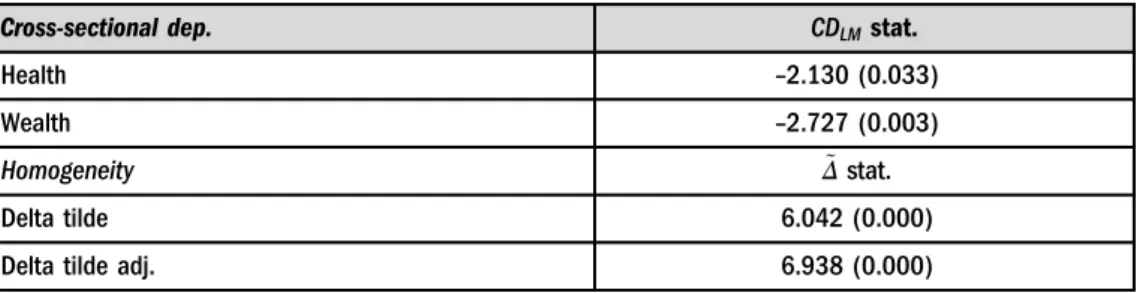
Cross-section dependency as a shock in one country affects other country/countries, and it can also be deﬁned as the existence of a correlation between units. In terms of the nature of the study, it is of great importance to investigate the probability that whether the shocks that occur in the variables of health and wealth affect other countries. In addition, if there is cross-section dependency, unit root tests that take into account the correlation between the units should be used. In the study, the cross-sectional dependence is examined with the help of the CD test, which can be used in the cases where the cross-section dimension (N) is greater than the time dimension (T). The null hypothesis of the CD test which claims that there is no relationship between the cross-sections is rejected for both health and wealth variables, and it is attained that there is a correlation among these countries.

Subsequently, the slope coefficients of the countries are tested for homogeneity by Delta tilde ðΔÞ~ and Delta tilde adjustðΔ~adjÞhomogeneity tests. As a result of the Delta tests, the null hypothesis which expresses the homogeneity of the slope coefﬁcients is rejected, whereas the slope

Table 3.Tests for the cross-sectional dependence and homogeneity

Cross-sectional dep. CDLMstat.

Health –2.130 (0.033)

Wealth –2.727 (0.003)

Homogeneity Δ~stat.

Delta tilde 6.042 (0.000)

Delta tilde adj. 6.938 (0.000)

Note: The probability values are in the parentheses.

(12)

coefﬁcients of the countries are heterogeneous. Theﬁndings of the CD and the Delta tests are given inTable 3.

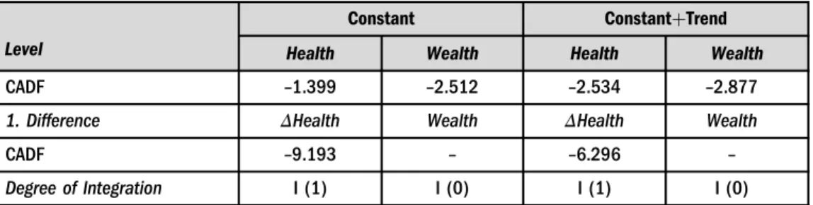
As a result of the CD test, the cross-section dependency of the variables is established, and the stability of the series is investigated using the CADF test, from the second generation unit root tests, which takes cross-section dependency into consideration. According to the CADF statistics (see in Table 4), while the health variable becomes stable in the ﬁrst difference, the wealth variable is found to be stable in the level.

After examining the data with preliminarily tests, the analysis is carried out with the Emirmahmutoglu–Kose (EK) test, which investigates heterogeneous panel causality. According to the results of the EK panel causality test (as seen in Table 5), while the countries where causality is determined from health to wealth are Albania, Bulgaria, Finland, Greece, Latvia, Macedonia, Poland, Turkey, Iceland, Bosnia-Herzegovina. Albania, Belgium, Croatia, Czech Republic, France, Germany, Hungary, Italy, Luxembourg, Poland, Portugal, United Kingdom and Norway, are those where causality is identiﬁed from wealth to health. Furthermore, according to the Fisher statistics in the EK test, there is a causality relationship from health to wealth and from wealth to health for the whole panel at the level of 1%.

InTable 6, according to the results of the causality test, the countries are listed in terms of whether there is a one-way or two-way causal relationship between health and wealth or no relationship at all. It has been determined that there are two countries with bi-directional causality both from health to wealth and from wealth to health, these countries are Poland and the EU candidate Albania. As seen inTable 6, there is a one-way causal relationship from wealth to health in 10 EU, and 1 EFTA countries. On the other hand, it is noteworthy that one-way causality from health to wealth is found in Bulgaria, Finland, Greece, Latvia, Macedonia, Turkey, Iceland and Bosnia-Herzegovina. In Austria, Cyprus, Denmark, Estonia, Ireland, Lithuania, Malta, Netherlands, Romania, Slovak Republic, Slovenia, Spain, Sweden, and Switzerland no causality is found. This group includes Switzerland as an EFTA country, while all other countries are the EU members.

As stated before, in the healthy and wealthy country clusters obtained by discriminant analysis, it is found that 17 countries are included in both groups. If it is compared with the findings obtained by the panel causality test, it is seen that from these countries Finland and

Table 4. The results of panel unit root tests

Level

Constant ConstantþTrend

Health Wealth Health Wealth

CADF –1.399 –2.512 –2.534 –2.877

1. Difference ΔHealth Wealth ΔHealth Wealth

CADF –9.193 – –6.296 –

Degree of Integration I (1) I (0) I (1) I (0)

Note: In the CADF test, the maximum lag length was taken as 3, and the optimal lag length was determined according to the Schwarz Criterion. The CADF panel statistical critical values for the with-constant model are –2.230,–2.110 and–2.040, and–2.730,–2.610 and–2.540 for the with-constant and trend model.

(13)

Table 5.The result of Emirmahmutoglu–Kose panel causality test

Hypothesis H0: Health≠>Wealth H0: Wealth≠>Health

Country Lag Statistics P-value Statistics P-value

Albania 3 7.803^p 0.050 9.448^pp 0.024

Austria 2 1.678 0.432 4.249 0.119

Belgium 3 0.299 0.960 6.647^p 0.084

Bosnia-Herzegovina 3 11.711^ppp 0.008 2.395 0.495

Bulgaria 2 6.820^pp 0.033 2.334 0.311

Croatia 1 0.732 0.392 5.163^pp 0.023

Cyprus 3 1.373 0.712 1.263 0.738

Czech Republic 2 0.490 0.783 7.862^pp 0.019

Denmark 2 0.078 0.962 1.482 0.477

Estonia 3 1.045 0.790 2.544 0.467

Finland 3 12.041^ppp 0.007 2.441 0.486

France 3 1.373 0.712 8.351^pp 0.039

Germany 2 0.634 0.728 6.737^pp 0.034

Greece 3 14.398^ppp 0.002 1.052 0.789

Hungary 3 1.353 0.717 10.371^pp 0.016

Iceland 2 5.236^p 0.073 1.321 0.517

Ireland 1 0.779 0.377 0.283 0.594

Italy 2 0.026 0.987 8.184^pp 0.017

Latvia 3 9.694^pp 0.021 0.828 0.843

Lithuania 2 2.040 0.361 1.525 0.467

Luxembourg 3 2.837 0.417 9.252^pp 0.026

Macedonia 3 7.035^p 0.071 1.465 0.690

Malta 3 1.584 0.663 3.842 0.279

Netherlands 2 0.556 0.757 4.114 0.128

Norway 2 1.215 0.545 6.954^p 0.074

Poland 3 9.047^pp 0.029 12.845^ppp 0.005

Portugal 2 0.940 0.625 5.374^p 0.068

Romania 3 2.252 0.522 3.120 0.373

Slovak Republic 2 1.813 0.404 1.403 0.495

Slovenia 1 0.108 0.743 0.168 0.682

(continued)

(14)

Iceland have a one-way causality from health to inclusive wealth. At the same time, one-way causality is established in Belgium, Czech Republic, France, Germany, Luxembourg, Norway and United Kingdom from wealth to health. However, a causality relationship has not been found for Austria, Cyprus, Denmark, Ireland, Netherlands, Slovenia, Sweden and Switzerland, which are both healthy and wealthy countries. Therefore, for these countries, it can be thought that being healthier does not originate from wealth, or being wealthier does not result from being healthier. As a result of discriminant analysis, 11 countries are located in both less healthy and less wealthy clusters. According to the panel causality test, among these countries, for Croatia, there is a one-way relationship from wealth to health while a two-way causality exists for Albania and Poland. There is also a one-way relationship from health to wealth for Latvia, Bulgaria, Macedonia, Bosnia-Herzegovina and Turkey.

Table 5. Continued

Hypothesis H0: Health≠>Wealth H0: Wealth≠>Health

Country Lag Statistics P-value Statistics P-value

Spain 2 1.480 0.477 2.992 0.224

Sweden 2 1.009 0.604 5.292 0.152

Switzerland 2 0.545 0.761 4.196 0.123

Turkey 3 13.321^ppp 0.004 2.279 0.516

United Kingdom 1 1.487 0.223 2.798^p 0.094

Fisher statistics 127.644^ppp 0.000 135.832^ppp 0.000

Note:^p,^pp,^ppprefer to a signiﬁcance level of 10%, 5% and 1%, respectively.

Table 6. Countries according to the causality results

Health¼>Wealth Wealth¼>Health Health<¼>Wealth No Causality Bosnia-Herzegovina

Bulgaria Finland Greece Iceland Latvia Macedonia Turkey

Belgium Croatia Czech Republic

France Germany

Hungary Italy Luxembourg

Norway Portugal United Kingdom

Albania Poland

Austria Cyprus Denmark

Estonia Ireland Lithuania

Malta Netherlands

Romania Slovak Republic

Slovenia Spain Sweden Switzerland

(15)

Albania and Poland with bi-directional causality as a result of the panel causality test are included in both the less healthy and less wealthy clusters obtained by the discriminant analysis.

It is noteworthy that 10 of the 11 countries with causality from wealth to health is in the healthy country group. Furthermore, it is pointed out that 6 out of 8 countries with causality from health to wealth are in the less wealthy group and 5 of them are both in the less healthy and less wealthy group.

5. CONCLUSION

Health is very important for humans’ well-being and happiness. It is commonly thought that healthier people live longer, their savings are higher, and they are also more productive, meaning that they can also contribute more to the development of the economy. Besides, it is suggested that in a better economy, people have a better quality and healthier life because their income is bigger and fair. Based on these ideas, one may ask whether human health is crucial in increasing the wealth of countries and whether the wealth of a country can decide the health of its citizens.

In this context, the present paper aims to reveal the causality relationship between health and inclusive wealth in the EU countries, the membership candidate states, and the EFTA countries between 1990 and 2015. The variables of health and inclusive wealth are dealt with more extensively according to the other works with macro data in the literature. 35 European countries are examined through comprehensive econometric analyses.

We divide the European countries into two clusters as healthy-less healthy and wealthy-less wealthy through the Two-step Cluster analysis. The binary variables attained by cluster analysis are taken as the dependent variables in the discriminant analysis, and then the health and wealth scores of each country for 1990–2015 are estimated. In these analyses, for the health variables mortality, life expectancy, sanitation, and tuberculosis rates are used, while GDP per capita, income inequality, employment rate and the mean years of schooling are applied for the wealth variables. According to the results, the healthiest country is Iceland and the least healthy is Romania, while the wealthiest and the least wealthy countries are found as Norway and Turkey, respectively. Besides, 73.9% of the countries that are in the healthy countries group are also included in the wealthy countries group, whereas about 91.7% of the less healthy countries group also includes those in the less wealthy category. These conclusions can be regarded as a prior demonstration of consistency in relation to the health-wealth relationship.

In the second stage, the causality between the variables of health and inclusive wealth is investigated first by theEmirmahmutoglu–Kose (2011)panel causality analysis. As a result, a two-way causality from wealth to health and from health to wealth is detected for the overall panel by the Fisher statistics. In addition, the EK test allowed country-speciﬁc causality results to be obtained. As a result of this test, a one-way causality can be determined in 11 cases as being from wealth to health, and in 8 the other way. The countries where the evidence of causality from wealth to health is detected in Belgium, Croatia, Czech Republic, France, Germany, Hungary, Italy, Luxembourg, Portugal, United Kingdom and Norway. Bulgaria, Finland, Greece, Latvia, Macedonia, Turkey, Iceland, and Bosnia-Herzegovina have a one-way causality from health to wealth. Furthermore, 14 out of 35 countries have no causality, whereas a two-way causality is found in 2 countries. Albania and Poland are the countries with bidirectional causality, both countries are included in the less healthy and less wealthy clusters as attained by

(16)

the discriminant analysis. Furthermore, according to the results, 90.9% of countries with causality from wealth to health are in the group of healthy countries. This result indicates that inclusive wealth is important to be healthy. In countries with higher inclusive wealth levels, healthy living and a healthy society are becoming a priority. It is noted that 5 out of 8 countries with causality from health to wealth are in both the less healthy and less wealthy groups. The importance these countries must give to health, which is a component of human capital, in order to become wealthy is remarkable.

It is known that health expenditures increase the productivity of the labor force and provide long-term returns. Health care, not only benefits labor productivity but also helps savings in future health expenditures as a result of reduction in diseases (Mushkin 1962;Grossman 1972).

In this context, health services and health expenditures are gaining importance. Besides, it should be taken into consideration that health sector transformation regarding private and public health expenditures, insurance coverage and health financing being more inclusive indirectly increase wealth. As for limitations, other relevant data such as cancer, diabetes, blood pressure, heart disease and perhaps mental illness, which are among the most important health problems of today, establish other important aspects of the subject and, as such, need to be dealt with extensively. However, because of the limited data, the health index was handled with the variables mentioned. Based on the findings, further elaboration of causality and more comprehensive research on the basis of each countries’ specific futures are recommended for future studies.

REFERENCES

Acemoglu, D.–Johnson, S. (2007): Disease and Development: The Effect of Life Expectancy on Economic Growth.Journal of Political Economy, 115(6): 925–985.

Adams, P.–Hurd, M. D.–McFadden, D.–Merrill, A.–Ribeiro, T. (2003): Healthy, Wealthy, and Wise?

Tests for Direct Causal Paths Between Health and Socioeconomic Status. Journal of Econometrics, 112(1): 3–56.

Aghion, P.–Howitt, P.–Murtin, F. (2010): The Relationship Between Health and Growth: When Lucas Meets Nelson Phelps.Working Paper, No. 15813. National Bureau of Economic Research.

Anderberg, M. R. (1973):Cluster Analysis for Applications(1st ed.).New York: Academic press.

Andersson, K. – Dickin, S. –Rosemarin, A. (2016): Towards “Sustainable” Sanitation: Challenges and Opportunities in Urban Areas.Sustainability, 8(12): 1–14.

Bacher, J.–Wenzig, K.–Vogler, M. (2004): SPSS TwoStep Cluster–A First Evaluation.Working paper, RC33 Sixth International Conference on Social Science Methodology: “Recent Developments and Applications in Social Research Methodology”, Amsterdam, The Netherlands, August 16–20.

Biggs, B.–King, L.–Basu, S.–Stuckler, D. (2010): Is Wealthier Always Healthier? The Impact of National Income Level, Inequality, and Poverty on Public Health in Latin America.Social Science&Medicine, 71(2): 266–273.

Bloom, D. E.–Canning, D.–Jamison, D. T. (2004): Health, Wealth, and Welfare.Finance and Devel- opment, 41: 10–15.

Breusch, T. S.–Pagan, A. R. (1980): The Lagrange Multiplier Test and Its Applications to Model Speci- ﬁcation in Econometrics.The Review of Economic Studies, 47(1): 239–253.

(17)

Brown, M. T.–Wicker, L. R. (2000): Discriminant Analysis.In: Tinsley, H. E. A.–Brown, S. D. (eds):

Handbook of Applied Multivariate Statistics and Mathematical Modeling. London: Academic Press, Ch. 8, pp. 209–235.

Deaton, A. (2002): Policy Implications of the Gradient of Health and Wealth.Health Affairs, 21(2): 13–30.

Deaton, A. (2007): Income, Aging, Health and Wellbeing Around the World: Evidence from the Gallup World.Working Paper, No. 13317. National Bureau of Economic Research.

Easton-Brooks, D.–Davis, A. (2007): Wealth, Traditional Socioeconomic Indicators, and the Achievement Debt.The Journal of Negro Education, 76(4): pp. 530–541.

Emirmahmutoglu, F.–Kose, N. (2011): Testing for Granger Causality in Heterogeneous Mixed Panels.

Economic Modelling, 28(3): 870–876.

European Comission (2016):Ninth Report on the Implementation Status and the Programmes for Imple- mentation (as required by Article 17) of Council Directive 91/271/EEC Concerning Urban Waste Water Treatment. https://eur–lex.europa.eu/legal–content/EN/TXT/PDF/?uri5CELEX:52017DC0749&

from5EN.

Everitt, B. S.–Landau, S.–Leese, M.–Stahl, D. (2011):Cluster Analysis(5th ed.). United Kingdom: John Wiley&Sons Ltd.

Fielding, D.–Torres, S. (2009): Health, Wealth, Fertility, Education, and Inequality.Review of Development Economics, 13(1): 39–55.

Fisher, R. A. (1936): The Use of Multiple Measurements in Taxonomic Problems.The Annals of Human Genetics, 7(2): 179–188.

Grossman, M. (1972): On the Concept of Health Capital and the Demand for Health.Journal of Political Economy, 80(2): 223–255.

Hair, J. F.–Black, W. C.–Babin, B. J.–Anderson, R. E. (2010):Multivariate Data Analysis: A Global Perspective.New Jersey: Pearson.

Hansen, C. W. (2012): The Relation between Wealth and Health: Evidence from a World Panel of Countries.Economics Letters, 115(2): 175–176.

Howitt, P. (2004): Endogenous Growth, Productivity and Economic Policy: A Progress Report.Interna- tional Productivity Monitor. Centre for the Study of Living Standards, 8: 3–15.

Kozun-Cieslak, G. (2020): Is the Efﬁciency of the Healthcare System Linked to the Country’s Economic Wealth? Beveridgeans versus Bismarckians.Acta Oeconomica, 70(1): 1–17.

Kunze, L. (2014): Life Expectancy and Economic Growth.Journal of Macroeconomics, 39: 54–65.

Lorentzen, P.–McMillan, J.–Wacziarg, R. (2008): Death and Development.Journal of Economic Growth, 13(2): 81–124.

Markou, G.–Palaiolouga, E.–Kokkinakos, P.–Markaki, O. I.–Koussouris, S.–Askounis, D. (2015):

Prosperity Indicators–A Landscape Analysis. EEPM@ eGOV.

Michaud, P. C. –van Soest, A. (2008): Health and Wealth of Elderly Couples: Causality Tests Using Dynamic Panel Data Models.Journal of Health Economics, 27(5): 1312–1325.

Mushkin, S. J. (1962): Health as an Investment.Journal of Political Economy, 70(5): 129–157.

Pesaran, M. H. (2004): General Diagnostic Tests for Cross Section Dependence in Anels.CESifo Working Paper Series, No. 1229; IZA Discussion Paper, No. 1240.

Pesaran, H. M. (2008): A Simple Panel Unit Root Test in the Presence of Cross Section Dependence.

Journal of Applied Econometrics, 22(2): 265–312.

Pesaran, M. H.–Yamagata, T. (2008): Testing Slope Homogeneity in Large Panels.Journal of Econometrics, 142(1): 50–93.

(18)

Pope, C. A., III–Ezzati, M.–Dockery, D. W. (2009): Fine-Particulate Air Pollution and Life Expectancy in the United States.The New England Journal of Medicine, 360(4): 376–386.

Pritchett, L.–Summers, L. H. (1996): Wealthier is Healthier.Journal of Human Resources, 31(4): 841–868.

Robine, J. M.–Ritchie, K. (1991): Healthy Life Expectancy: Evaluation of Global Indicator of Change in Population Health.BMJ, 302(6774): 457–460.

Roman, P.–Thiry, G. (2016). The Inclusive Wealth Index. A Critical Appraisal.Ecological Economics, 124:

185–192.

Rundle-Thiele, S.–Kubacki, K.–Tkaczynski, A.–Parkinson, J. (2015): Using Two-Step Cluster Analysis to Identify Homogeneous Physical Activity Groups.Marketing Intelligence&Planning, 33(4): 522–537.

Sarstedt, M.–Mooi, E. (2011):A Concise Guide to Market Research: The Process, Data, and Methods Using IBM SPSS Statistics.Berlin Heidelberg: Springer Verlag.

Sharma, S. (1996):Applied Multivariate Techniques. John Wiley&Sons.

Solt, F. (2014): The Standardized World Income Inequality Database.Working Paper, SWIID Version 5.0.

Somoskovi, A.–Ahmedov, S.–Salﬁnger, M. (2013): It is Health that is Real Wealth & Not Pieces of Gold

& Silver.The Indian Journal of Medical Research, 137(3): 437–439.

Tabachnick, B. G.–Fidell, L. S. (2003).Using Multivariate Statistics(6th edition). USA: Pearson Education.

United Nations: The Sustainable Development Goals (SDGs).http://www.un.org/sustainabledevelopment/

health.

UNU–IHDP –UNEP (2014): Inclusive Wealth Report 2014. Measuring Progress toward Sustainability.

Summary for Decision-Makers. Delhi: UNU–IHDP.

Wilkinson, R. G.–Pickett, K. E. (2008): Income Inequality and Socioeconomic Gradients in Mortality.

American Journal of Public Health, 98(4): 699–704.

World Bank Development Indicators.http://data.worldbank.org/indicator.

World Health Organization, Regional Ofﬁce for Europe (2019):Tuberculosis Surveillance and Monitoring in Europe 2019: 2017 Data.https://apps.who.int/iris/handle/10665/311349.