Markov modeling of traffic flow in Smart Cities ∗
Norbert Bátfai, Renátó Besenczi, Péter Jeszenszky, Máté Szabó, Márton Ispány
Faculty of Informatics, University of Debrecen, Hungary besenczi.renato@inf.unideb.hu
jeszenszky.peter@inf.unideb.hu szabo.mate@inf.unideb.hu ispany.marton@inf.unideb.hu
Submitted: January 15, 2021 Accepted: April 25, 2021 Published online: May 18, 2021
Dedicated to the kind memory of our colleague, Norbert Bátfai.
Abstract
Modeling and simulating the traffic flow in large urban road networks are important tasks. A mathematically rigorous stochastic model proposed in [8]
is based on the synthesis of the graph and Markov chain theories. In this model, the transition probability matrix describes the traffic dynamics and its unique stationary distribution approximates the proportion of the vehicles at the segments of the road network. In this paper various Markov models are studied and a simulation method is presented for generating random traffic trajectories on a road network based on the two-dimensional stationary distribution of the models. In a case study we apply our method to the central region of the city of Debrecen by using the road network data from the OpenStreetMap project which is available publicly.
∗Renátó Besenczi and Márton Ispány are supported by Project no. TKP2020-NKA-04 which has been implemented with the support provided from the National Research, Development and Innovation Fund of Hungary, financed under the 2020-4.1.1-TKP2020 funding scheme. Péter Jeszenszky and Máté Szabó are supported by the EFOP-3.6.1-16-2016-00022 project. The project is co-financed by the European Union and the European Social Fund.
doi: https://doi.org/10.33039/ami.2021.04.008 url: https://ami.uni-eszterhazy.hu
21
Keywords:Road network, traffic simulation, discrete time Markov chain, sta- tionary distribution, OpenStreetMap
1. Introduction
Recently, the research and development of Smart City applications have become more important by providing services to inhabitants which can make everyday life easier [15]. These applications are based on emerging technologies such as big data analytics, cloud computing, and complex sensor systems (IoT) that can support their operation. By the year 2050, 70% of Earth’s population is expected to live in cities [5] whose infrastructures will face new challenges, e.g., in the field of urban traffic. In the past few years, many developments have occurred in the automobile industry, e.g., autonomous (driverless) and pure electric cars are being introduced.
Since more and more people live in urban areas, solutions for problems of dense traffic such as air pollution and congestion are highly demanding [20, 24, 30].
This research presented in this paper follows our development of a traffic sim- ulation platform initiative called rObOCar World Championship (or OOCWC for short) [2, 3]. OOCWC is a multiagent-oriented environment for creating urban traffic simulations. The traffic simulations are performed by one of its components called Robocar City Emulator (RCE), which is an open source software released un- der the GNU GPL v3 and is available on GitHub.1 RCE uses the OpenStreetMap (OSM) database and processes it with the Osmium Library. The traffic simulation model of RCE is based on the Nagel-Schreckenberg (NaSch) model [21]. The re- sult of this processing is a routing map graph and a Boost Graph Library graph which can be visualized by various map viewers. For a detailed description of the operation of RCE, see [2]. There exist several traffic simulation platforms, e.g., Multi-Agent Transport Simulation [14], Simulation of Urban Mobility [18], Aimsun,2 and PTV Vissim3. The main focus of their simulation algorithms is on microscopic traffic events, while our software system focuses only on the traffic flow on the road network of the whole city.
In [8] a mathematically rigorous stochastic model is proposed for investigating the traffic flow on a road network which is based on the synthesis of discrete time Markov chains and graph theory. In this model the transition probability matrix describes the dynamics of the traffic while its unique stationary distribution cor- responds to the traffic equilibrium (or steady) state on the road network. In our previous paper [4], the concepts of Markov traffic and two-dimensional stationary distribution are introduced and a parameter estimation method is proposed by us- ing the weighted least squares (WLS) approach. To investigate complex systems, the joint application of Markov chains and large graphs is well known, see [7, 10, 19].Our contributions in this paper are as follows. Using the approach in [4], we
1https://github.com/nbatfai/robocar-emulator
2https://www.aimsun.com/
3http://vision-traffic.ptvgroup.com/en-us/products/ptv-vissim/
present various Markov models for modeling traffic flow on different road graph models based on, e.g., open or closed and digraph or line digraph views. We prove the existence and uniqueness of a stationary distribution as a solution of the global balance equation, see Theorem 3.1. We define the configuration space of Markov traffic, describe the transition mechanism and prove the ergodicity of Markov traffic, see Theorem 4.1. Finally, we propose a simulation method for gen- erating random trajectories for a Markov traffic whose two-dimensional distribution is closest to a prescribed mask matrix in the least squares sense, see Theorem 5.1.
The results of this paper together with those obtained in [4], which contains some additional proofs, show that the Markovian approach still works when the scale of the road graph is significantly enlarged compared to such small one as ‘De Uithof’, which is a district in the city of Utrecht in Netherlands, see [11].
Several approaches exist for traffic flow simulation and prediction, some recent surveys are [22, 27, 31], but a few of them are based on Markov models, see [8, 23].
This paper is structured as follows. In section 2 we present various graph models of road networks. Section 3 is devoted to the probability distributions and Markov kernels on road networks. Section 4 introduces the notion of Markov traffic, describes its stationary distribution and proves its ergodicity. A simulation method is presented in section 5. In section 6 we discuss our findings, and in section 7 we conclude the paper. The Appendix provides a toy example and a proof.
2. Graph modeling of road networks
Recall that the ordered pair 𝐺 = (𝑉, 𝐸) is a directed graph (digraph), where 𝑉 is a finite set of vertices and 𝐸 is a set of ordered pairs, called directed edges, of vertices. In the sequel, vertices (or nodes) are denoted by𝑢, 𝑣, 𝑤,edges (or arcs or arrows) are denoted by𝑒, 𝑓, 𝑔. For a directed edge𝑒= (𝑣, 𝑤)∈𝐸 we also use the notation𝑣 →𝑤. We suppose that 𝐺is a simple digraph, i.e., it does not contain multiple arrows. For details, see the textbook [1].
A road network𝐺is defined as a simple directed graph, 𝐺= (𝑉, 𝐸), where 𝑉 is a set of nodes representing the terminal points of road segments, and𝐸 is a set of directed edges denoting road segments, see [25]. A road segment𝑒= (𝑣, 𝑤)∈𝐸 is a directed edge in a road network graph, with two terminal points𝑣and𝑤. The vehicles move on this edge from𝑣 to𝑤. The road network𝐺represents the road system of a city.
Let𝑆 denote the diagonal set of𝑉, i.e.,𝑆:={(𝑣, 𝑣)|𝑣 ∈𝑉}. From a practical point of view, we suppose that 𝐸∩𝑆=∅, i.e., there is no loop𝑣 →𝑣 in the road network in order to avoid that a vehicle is able to move in an infinite cycle. For 𝑣∈𝑉, define𝑣− :={𝑒∈𝐸| ∃𝑢∈𝑉 :𝑒= (𝑢, 𝑣)}and𝑣+ :={𝑒∈𝐸| ∃𝑤∈𝑉 :𝑒= (𝑣, 𝑤)}, i.e., 𝑣− and 𝑣+ are the sets of edges in and out the node𝑣, respectively.
Then, 𝑑𝑒𝑔−(𝑣) =|𝑣−| and𝑑𝑒𝑔+(𝑣) =|𝑣+|are the indegree and outdegree of node 𝑣, respectively.
Let L(𝐺) = (𝑉′, 𝐸′)be the line digraph (line road network, network line graph, see [9]) associated to𝐺, see Section 4.5 in [1]. Here,𝑉′=𝐸and the set𝐸′ consists
of the ordered pairs (𝑒, 𝑓) where 𝑒, 𝑓 ∈ 𝐸 such that there exist 𝑢, 𝑣, 𝑤 ∈ 𝑉 that 𝑒 = (𝑢, 𝑣) and 𝑓 = (𝑣, 𝑤), i.e., 𝑢 → 𝑣 → 𝑤 is a path of length 2 (dipath) in 𝐺. The elements of 𝐸′ can be described by triplets (𝑢, 𝑣, 𝑤), where 𝑢, 𝑣, 𝑤 ∈𝑉, (𝑢, 𝑣),(𝑣, 𝑤) ∈ 𝐸, and for a directed edge in L(𝐺) we use the notation (𝑢, 𝑣) → (𝑣, 𝑤)too.
The digraph model of a road network assigns the vehicles moving in a city to the vertices (first-order or primal network). Contrarily, the line digraph model assigns the vehicles to the edges (second-order or dual network), see [26, 29]. When we are studying issues that are associated with the crossings (vertices) we will be concerned with the adjacency relationships of crossings, and so with the road network. On the other hand, when we are studying issues that associated with road segments we will be concerned with the adjacency relationships of road segments, and so our analyses will involve the line road network.
The digraphs 𝐺 and L(𝐺)can be characterized by their degree distributions.
The pairs (𝑖, 𝑛+𝑖 ) form the frequency histogram for the outdegree distribution of 𝐺 where 𝑛+𝑖 := |{𝑣 ∈ 𝑉 |𝑑𝑒𝑔+(𝑣) = 𝑖}|. The indegree frequency histogram can be defined similarly as (𝑖, 𝑛−𝑖 ), where 𝑛−𝑖 := |{𝑣 ∈ 𝑉 |𝑑𝑒𝑔−(𝑣) = 𝑖}|. The pairs (𝑖, 𝑚+𝑖 )form the frequency histogram for the outdegree distribution of L(𝐺)where 𝑚+𝑖 := ∑︀
𝑣∈𝐺+𝑖 𝑑𝑒𝑔−(𝑣) and 𝐺+𝑖 := {𝑣 ∈ 𝑉|𝑑𝑒𝑔+(𝑣) = 𝑖}. (Note that 𝑛+𝑖 =
|𝐺+𝑖 |.) Similarly, the pairs(𝑖, 𝑚−𝑖 ) form the frequency histogram for the indegree distribution of L(𝐺)where 𝑚−𝑖 :=∑︀
𝑣∈𝐺−𝑖 𝑑𝑒𝑔+(𝑣)and𝐺−𝑖 :={𝑣∈𝑉 |𝑑𝑒𝑔−(𝑣) = 𝑖}. For the city of Debrecen (described later in this paper), the above mentioned degree distributions can be seen in Fig. 6. These histograms corroborate the fact that Debrecen’s road network is a sparse graph since there is no node with higher in- and outdegree than 4.
Recall that a sequence 𝑣1, . . . , 𝑣ℓ ∈ 𝑉, ℓ ∈ N, is called walk of length ℓ if 𝑣1 →𝑣2 → · · · → 𝑣ℓ. A walk is called path if its elements are different vertices.
For a pair 𝑢, 𝑣 ∈ 𝑉, 𝑢 ̸= 𝑣, it is said that 𝑣 is reachable from 𝑢if there exists a walk 𝑣1, 𝑣2, . . . , 𝑣ℓ such that𝑢=𝑣1 and𝑣 =𝑣ℓ. Clearly, if𝑣 is reachable from𝑢, then there is a path from 𝑢 to 𝑣. A digraph 𝐺 is said to be strongly connected (diconnected) if every vertex is reachable from every other vertex. Clearly, the line digraph of a strongly connected digraph is also strongly connected. Namely, if𝑒= (𝑢, 𝑣)∈𝑉′(= 𝐸)and𝑓 = (𝑤, 𝑧)∈𝑉′ are arbitrary such that 𝑒̸=𝑓, then, since 𝐺 is strongly connected, there exists a walk (or a path) of length ℓ in 𝐺 such that 𝑣 =𝑣1 →𝑣2 →. . . →𝑣ℓ =𝑤, where 𝑣1, . . . , 𝑣ℓ ∈𝑉, and thus we have 𝑒 = (𝑢, 𝑣) → (𝑣1, 𝑣2) → . . . → (𝑣ℓ−1, 𝑣ℓ) → (𝑤, 𝑧) = 𝑓, i.e., there exists a walk (or a path) of length ℓ in L(𝐺) between the vertices 𝑒, 𝑓 ∈ 𝑉′. If 𝑢 → 𝑣 → 𝑢 for a pair 𝑢, 𝑣 ∈ 𝑉 then we have (𝑢, 𝑣) → (𝑣, 𝑢) → (𝑢, 𝑣) in the line digraph, i.e., vehicles can turn back at vertex 𝑢 into 𝑣. Sometimes the traffic regulations do not allow this kind of reversal, i.e., the edge set 𝐸′ in L(𝐺) must not contain some triplet(𝑢, 𝑣, 𝑢), while some of these triplets are needed that L(𝐺)be strongly connected. By deleting all of the unnecessary triplets(𝑢, 𝑣, 𝑢),𝑢, 𝑣∈𝑉, such that the remaining line digraph be still strongly connected we get the minimal strongly connected line digraph of𝐺. This line digraph is denoted by ML(𝐺). For example,
the vertices of ML(𝐺)for𝐺in Fig. 1 are given in Table 1.
Recall that a cycle𝐶 ⊂𝑉 in digraph𝐺is a path 𝑣1 →𝑣2 →. . . →𝑣ℓ → 𝑣1. Here ℓ(𝐶) =ℓis called the length of𝐶. A digraph𝐺is said to be aperiodic if the greatest common divisor of the lengths of its cycles is one. Formally, the period of 𝐺is defined as𝑝𝑒𝑟(𝐺) := gcd{ℓ >0 :∃𝐶⊂𝑉 cycle such thatℓ(𝐶) =ℓ}. Then,𝐺 is called aperiodic if𝑝𝑒𝑟(𝐺) = 1. Clearly, if a digraph𝐺is aperiodic then its line digraph L(𝐺) is also aperiodic. This statement follows from the following fact: if 𝑣1 →𝑣2 → . . . →𝑣ℓ →𝑣1 is a cycle then(𝑣1, 𝑣2)→ (𝑣2, 𝑣3)→ . . . →(𝑣ℓ, 𝑣1) → (𝑣1, 𝑣2)is a cycle in L(𝐺). Thus, ifℓ >0and there exists a cycle𝐶⊂𝑉 such that ℓ(𝐶) =ℓthen there exists a cycle𝐶′⊂𝑉′ such thatℓ(𝐶′) =ℓ.
3: 2/11
2: 4/11
1: 2/11 4: 2/11
5: 1/11 1/2
1/2
1/4 1/4
1/2
1/2 1/2
1/4 1/4
1/2 1/2
1/2
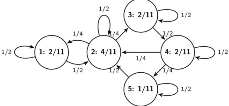
Figure 1. A Markov kernel (on edges) with its stationary distri- bution (on vertices with node’s id) on a simple road network.
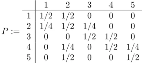
Table 1. An example for a Markov kernel on the minimal line digraph of the road network in Fig. 1.
(1,2) (2,3) (3,4) (4,2) (2,1) (4,5) (5,2)
(1,2) 1/2 1/2 0 0 0 0 0
(2,3) 0 1/2 1/2 0 0 0 0
(3,4) 0 0 1/2 1/4 0 1/4 0
(4,2) 0 1/4 0 1/2 1/4 0 0
(2,1) 1/2 0 0 0 1/2 0 0
(4,5) 0 0 0 0 0 1/2 1/2
(5,2) 0 1/4 0 0 1/4 0 1/2
Let𝐴= (𝑎𝑢𝑣)𝑢,𝑣∈𝑉 denote the adjacency matrix of the digraph𝐺, i.e.,𝑎𝑢𝑣= 1 if and only if (𝑢, 𝑣) ∈ 𝐸 and 0 otherwise. The number of directed walks from vertex 𝑢to vertex𝑣 of length 𝑘is the entry in the𝑢-th row and the𝑣-th column of the matrix 𝐴𝑘. For example, in Fig. 1, the number of directed walks of length 6 from vertex 2 to vertex 4 is 2, see Appendix 7. One can easily check that 𝐺 is strongly connected if and only if there is a positive integer𝑘such that the matrix 𝐼+𝐴+· · ·+𝐴𝑘 is positive, i.e., all the entries of this matrix are positive. The
indegree and outdegree of a vertex 𝑣 can be expressed by the adjacency matrix as 𝑑𝑒𝑔−(𝑣) =∑︀
𝑢∈𝑉 𝑎𝑢𝑣 and 𝑑𝑒𝑔+(𝑣) =∑︀
𝑢∈𝑉 𝑎𝑣𝑢. Let us introduce the vectors 𝑑− := (𝑑𝑒𝑔−(𝑣))𝑣∈𝑉 and 𝑑+ := (𝑑𝑒𝑔+(𝑣))𝑣∈𝑉. Then, we have 𝑑− = 𝐴𝑇1 and 𝑑+ =𝐴1where 1:= (1)𝑣∈𝑉 is the constant unit function. It is well known that the adjacency matrix 𝐴of an aperiodic, strongly connected graph 𝐺is primitive, i.e., irreducible and has only one eigenvalue of maximum modulus. Primitivity is equivalent to the following quasi-positivity: there exists𝑘∈Nsuch that the matrix 𝐴𝑘 >0, see Section 8.5 in [13].
In order to model the cases when vehicles leave or enter the city, we augment𝑉 by a new ideal vertex 0 and define𝑉 :=𝑉 ∪ {0}, see [12]. Moreover, let𝐸denote the augmentation of𝐸by directed edges(0, 𝑣)and(𝑣,0)for getting into and out of the city, respectively. Note that, for𝐸, it is not allowed to contain the loop(0,0).
The augmentation 𝐺 = (𝑉 , 𝐸)of 𝐺 is called the closure of the road network 𝐺.
For 𝑒= (𝑣, 𝑤)∈𝐸 we also use the notation 𝑣 →𝑤. In what follows, we suppose that there exist𝑢, 𝑣∈𝑉 such that𝑢→0and0→𝑣.
Each definition, including strong connectedness, periodicity, line digraph, given for 𝐺 can be extended for 𝐺 in a natural way. Note that in the augmented line digraph L(𝐺) = (𝑉′, 𝐸′)the elements of the edge set𝐸′can be described by triplets (𝑢, 𝑣, 𝑤), where𝑢, 𝑣, 𝑤∈𝑉 and if𝑣= 0then𝑢, 𝑤̸= 0and if𝑢or𝑤is 0 then𝑣̸= 0 because triplets(0,0, 𝑣),(𝑣,0,0), and(0,0,0)are excluded from𝐸′. One can easily see that if 𝐺 is strongly connected then its closure 𝐺 is also strongly connected.
Moreover, the strongly connected components of 𝐺, if there exist more than 1, can be connected through the ideal vertex 0, resulting in a strongly connected 𝐺.
Thus, the augmented line digraph will also be strongly connected. Clearly, if G is aperiodic then𝐺is aperiodic too.
In the rest of this paper, it is assumed that the road network is closed by augmenting with the ideal vertex 0.
3. Probability distributions and Markov kernels on road networks
On a road network, two kinds of probability distributions can be defined by consid- ering the set𝑉 or𝐸 as the state space, respectively. However, the Markov kernels on the line road network must be defined with particular care.
A probability distribution (p.d.) on𝑉 is the vector𝜋:= (𝜋𝑣)𝑣∈𝑉 where𝜋𝑣≥0 for all 𝑣 ∈ 𝑉 and ∑︀
𝑣∈𝑉 𝜋𝑣 = 1. We may think of 𝜋𝑣 as the proportion of all vehicles which drive through the crossing𝑣 with respect to all vehicles in the city.
A Markov kernel or transition probability matrix on𝑉 is defined as a real kernel 𝑃 := (𝑝𝑢𝑣)𝑢,𝑣∈𝑉 such that𝑝𝑢𝑣≥0for all𝑢, 𝑣∈𝑉 and∑︀
𝑣∈𝑉 𝑝𝑢𝑣= 1for all𝑢∈𝑉. The quantity𝑝𝑢𝑣∈[0,1]is called the transition probability from vertex𝑢to vertex 𝑣. In fact,𝑃 is a stochastic matrix on𝑉 and we assume that its support is the set
𝐸∪𝑆. The sum condition for Markov kernel𝑃 can be rewritten as:
∑︁
𝑤:𝑣→𝑤
𝑝𝑣𝑤+𝑝𝑣𝑣 = 1, 𝑣∈𝑉. (3.1)
A p.d.𝜋 is a stationary distribution (s.d.) of the kernel𝑃 if∑︀
𝑢∈𝑉 𝜋𝑢𝑝𝑢𝑣=𝜋𝑣
for all𝑣∈𝑉. This so-called global balance equation can be expressed as:
∑︁
𝑢:𝑢→𝑣
𝜋𝑢𝑝𝑢𝑣+𝜋𝑣𝑝𝑣𝑣 =𝜋𝑣, 𝑣∈𝑉. (3.2) Fig. 1 presents a Markov kernel with its s.d. on a simple road network.
Since the vehicles are moving along the road segments of the road network𝐺, it is natural to choose𝐸 to be the state space. In this case, to define probability distributions on the set of vertices again, we have to consider the line digraph L(𝐺) (or ML(𝐺)). Formally, a probability distribution (p.d.) on L(𝐺) is the vector 𝜋′ := (𝜋𝑒′)𝑒∈𝐸 where 𝜋𝑒′ ≥ 0 for all 𝑒 ∈ 𝐸 and ∑︀
𝑒∈𝐸𝜋′𝑒 = 1. If we want to emphasize the vertices of the original road network 𝐺, instead of the edges, then the notation 𝜋′𝑒=𝜋𝑢𝑣′ is also used where 𝑒= (𝑢, 𝑣)∈𝐸. We may think of 𝜋𝑒′ as the proportion of the vehicles at the road segment𝑒with respect to all vehicles in the city. Note that𝐺endowed with𝜋′ is a weighted digraph which is often called a network in itself as well.
A transition probability matrix (or Markov kernel) on𝐸, i.e., on the line digraph L(𝐺), can be defined as a real kernel 𝑃′ := (𝑝′𝑒𝑓)𝑒,𝑓∈𝐸 such that 𝑝′𝑒𝑓 ≥0 for all 𝑒, 𝑓 ∈𝐸and∑︀
𝑓∈𝐸𝑝′𝑒𝑓 = 1for all𝑒∈𝐸. A p.d.𝜋′ on𝐸is a s.d. of the kernel𝑃′if
∑︀
𝑒∈𝐸𝜋′𝑒𝑝′𝑒𝑓=𝜋′𝑓 for all𝑓 ∈𝐸. Since𝐺represents a road system we may suppose that if𝑒̸=𝑓 then𝑝′𝑒𝑓>0implies that(𝑒, 𝑓)∈𝐸′, i.e., there exist𝑢, 𝑣, 𝑤∈𝑉 such that𝑒= (𝑢, 𝑣)and𝑓 = (𝑣, 𝑤), and hence,𝑢→𝑣→𝑤is a walk of length 2. In this case, we use the notation𝑝′𝑒𝑓=𝑝′𝑢𝑣𝑤as well. In fact,𝑝′𝑢𝑣𝑤 denotes the probability that a vehicle on the road segment(𝑢, 𝑣)will go further to the road segment(𝑣, 𝑤) in the next time point. Moreover, in the case of𝑒 =𝑓 = (𝑢, 𝑣), let𝑝′𝑒𝑒 =𝑝′𝑢𝑣 be the probability that a vehicle remains on the same road segment in the next time point which can be non-zero as well. Thus, since𝑃′ is a Markov kernel, we have that, for all𝑢→𝑣, ∑︁
𝑤:𝑣→𝑤
𝑝′𝑢𝑣𝑤+𝑝′𝑢𝑣= 1 (3.3)
and the global balance equation is given as:
∑︁
𝑢:𝑢→𝑣
𝜋′𝑢𝑣𝑝′𝑢𝑣𝑤+𝜋′𝑣𝑤𝑝′𝑣𝑤=𝜋′𝑣𝑤 (3.4) for all𝑣→𝑤.
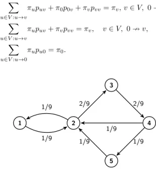
An example for the Markov kernel𝑃′ on the minimal line digraph ML(𝐺) of the road network𝐺in Fig. 1 is shown in Table 1. Fig. 2 shows the unique s.d. 𝜋′ of the Markov kernel 𝑃′.
Probability distributions and Markov kernels on the closure𝐺of an open road network𝐺can be defined similarly by considering the set𝑉 or𝐸as the state space,
respectively. Note that𝜋0 denotes the proportion of the number of vehicles which drive in or out of the city’s roads at a time point. Moreover, for any Markov kernel 𝑃 on𝑉 it is supposed that𝑝00= 0, i.e., the vehicles cannot move from 0 to 0, thus they either enter to the road network or leave the road network. Equations (3.1) and (3.2) remain true, too. Equation (3.1) can be rewritten as
∑︁
𝑤∈𝑉:𝑣→𝑤
𝑝𝑣𝑤+𝑝𝑣0+𝑝𝑣𝑣= 1, 𝑣∈𝑉,
∑︁
𝑤∈𝑉:0→𝑤
𝑝0𝑤= 1.
The global balance equation (3.2) for the s.d. can be rewritten as
∑︁
𝑢∈𝑉:𝑢→𝑣
𝜋𝑢𝑝𝑢𝑣+𝜋0𝑝0𝑣+𝜋𝑣𝑝𝑣𝑣 =𝜋𝑣, 𝑣∈𝑉, 0→𝑣,
∑︁
𝑢∈𝑉:𝑢→𝑣
𝜋𝑢𝑝𝑢𝑣+𝜋𝑣𝑝𝑣𝑣=𝜋𝑣, 𝑣∈𝑉, 09𝑣,
∑︁
𝑢∈𝑉:𝑢→0
𝜋𝑢𝑝𝑢0=𝜋0.
3
2
1 4
5 1/9
1/9 2/9 2/9
1/9
1/9 1/9
Figure 2. The stationary distribution of the Markov kernel in Table 1.
We can define Markov kernels on the line digraph L(𝐺)of the augmented road network 𝐺, and thus on the augmented edge set𝐸 similarly to the case of L(𝐺).
Note that (𝑒, 𝑓) ∈ 𝐸′ implies that 𝑒 = (𝑢, 𝑣) and 𝑓 = (𝑣, 𝑤) where 𝑢, 𝑣, 𝑤 ∈ 𝑉 excluding the triplets(0,0, 𝑣),(𝑣,0,0), and(0,0,0). We shall also use the notation 𝑝′𝑢𝑣𝑤=𝑝′𝑒𝑓 if𝑒= (𝑢, 𝑣)and𝑓 = (𝑣, 𝑤)and𝑝′𝑢𝑣=𝑝′𝑒𝑒 if𝑒= (𝑢, 𝑣). However, three additional conditions should be added. The first one is that𝑝′𝑢0𝑢= 0for all𝑢∈𝑉 such that 𝑢 →0 →𝑢. This means that if a vehicle is on the edge (𝑢,0), i.e., it leaves the city at vertex 𝑢 then it cannot be on the edge (0, 𝑢) at the next time point, i.e., it cannot enter at vertex𝑢in the road network again, immediately. The second one is that 𝑝′0𝑣0 = 0 for all 𝑣 ∈𝑉 such that0 →𝑣 →0, i.e., vehicles can
enter and leave the city at node 𝑣. This means that if a vehicle enters the city then it cannot leave the city at the next time point. Finally, the third one is that 𝑝′𝑢0=𝑝′0𝑣= 0for all𝑢, 𝑣∈𝑉 such that𝑢→0and0→𝑣. That is a vehicle cannot remain on the road network at the edge (𝑢,0) after two consecutive time points and if a vehicle enters into the road network at the edge(0, 𝑣)(or at the vertex𝑣) the first time then it does not remain on this edge after the next time point and it goes further immediately in the road network. Under these conditions, equations (3.3) and (3.4) remain true. Equation (3.3) can be rewritten as:
∑︁
𝑤∈𝑉:𝑣→𝑤
𝑝′𝑢𝑣𝑤+𝑝′𝑢𝑣0+𝑝′𝑢𝑣 = 1, 𝑢, 𝑣∈𝑉, 𝑢→𝑣,
∑︁
𝑤∈𝑉:𝑣→𝑤
𝑝′0𝑣𝑤= 1, 𝑣∈𝑉, 0→𝑣,
∑︁
𝑣∈𝑉∖{𝑢}:0→𝑣
𝑝′𝑢0𝑣= 1, 𝑢∈𝑉, 𝑢→0.
Equation (3.4) can be rewritten as:
∑︁
𝑢∈𝑉:𝑢→𝑣
𝜋𝑢𝑣′ 𝑝′𝑢𝑣𝑤+𝜋′0𝑣𝑝′0𝑣𝑤+𝜋𝑣𝑤′ 𝑝′𝑣𝑤=𝜋𝑣𝑤′ , 𝑣, 𝑤∈𝑉, 𝑣→𝑤,
∑︁
𝑢∈𝑉:𝑢→𝑣
𝜋𝑢𝑣′ 𝑝′𝑢𝑣0+𝜋′𝑣0𝑝′𝑣0=𝜋′𝑣0, 𝑣∈𝑉, 𝑣→0,
∑︁
𝑢∈𝑉∖{𝑤}:𝑢→0
𝜋𝑢𝑣′ 𝑝′𝑢0𝑤+𝜋0𝑤′ 𝑝′0𝑤=𝜋′0𝑤, 𝑤∈𝑉, 0→𝑤.
The s.d. in all cases, i.e., for Markov kernels on road networks, line road networks and their closures, can be derived by solving the above appropriate linear equations numerically. It turns out that there is a direct connection between the existence and uniqueness of s.d. of the Markov kernels𝑃 and𝑃′ and the strongly connected property of the physical road network 𝐺 if the Markov and graph structures are compatible with each other.
The Markov kernel𝑃 on𝑉 is called𝐺-compatible if, for any𝑢, 𝑣 ∈𝑉 such that 𝑢̸=𝑣, 𝑝𝑢𝑣 >0 if and only if(𝑢, 𝑣)∈𝐸. Similarly, the Markov kernel𝑃′ on𝐸 is called 𝐺-compatible if it is L(𝐺)-compatible Markov kernel on L(𝐺), i.e., for any 𝑒, 𝑓 ∈𝐸 such that𝑒̸=𝑓, 𝑝′𝑒𝑓 >0 if and only if(𝑒, 𝑓)∈𝐸′. This is equivalent to the statement that 𝑝′𝑢𝑣𝑤 > 0, 𝑢, 𝑣, 𝑤 ∈𝑉, if and only if (𝑢, 𝑣),(𝑣, 𝑤)∈𝐸. Since (𝑒, 𝑓)∈𝐸′if and only if there exist𝑢, 𝑣, 𝑤∈𝑉 such that𝑒= (𝑢, 𝑣)and𝑓 = (𝑣, 𝑤) we can define the𝐺-compatibility of a Markov kernel𝑃′ as, for any𝑒, 𝑓 ∈𝐸 such that 𝑒̸=𝑓, 𝑝′𝑒𝑓 >0 if and only if there exist𝑢, 𝑣, 𝑤∈𝑉 such that𝑒= (𝑢, 𝑣) and 𝑓 = (𝑣, 𝑤).
Clearly, if𝑃 is𝐺-compatible then the strong connectivity of𝐺implies that the Markov kernel (the transition matrix)𝑃 is irreducible. Thus, by Theorem 1 in [16], see also Theorem 3.1 and 3.3 in Chapter 3 of [6] the following theorem holds.
Theorem 3.1. If a road network𝐺is strongly connected then there is a unique sta- tionary distribution𝜋 (𝜋′) to any 𝐺-compatible Markov kernel𝑃 (𝑃′). Moreover, this distribution satisfies𝜋𝑣>0 for all𝑣∈𝑉 (𝜋′𝑢𝑣 >0 for all (𝑢, 𝑣)∈𝐸).
The main consequence of this theorem is that, in case of any physical road network augmented by the ideal vertex 0, all of the Markov kernels defined on the road network that has positive transition probability on all roads have unique s.d.
4. Markov traffic on road networks
Let(Ω,𝒜,P)be a probability space. A sequence{𝑋𝑡}𝑡∈Z+ of𝑉-valued r.v.’s is a Markov chain on the state space𝑉 if the Markov property holds:
P(𝑋𝑡=𝑣𝑡|𝑋𝑡−1=𝑣𝑡−1, . . . , 𝑋0=𝑣0) =P(𝑋𝑡=𝑣𝑡|𝑋𝑡−1=𝑣𝑡−1)
for all 𝑡∈N, 𝑣0, . . . , 𝑣𝑡∈𝑉. If 𝑋, 𝑋′ are𝑉-valued r.v.’s then for the conditional distribution𝑃 = (𝑝𝑣𝑣′)𝑣,𝑣′∈𝑉, 𝑝𝑣𝑣′ :=P(𝑋 =𝑣|𝑋′ =𝑣′), 𝑣, 𝑣′ ∈𝑉, we shall also use the notation𝑋|𝑋′. Clearly,𝑋|𝑋′is a Markov kernel on𝑉. Similarly, a Markov chain {𝑌𝑡}𝑡∈Z+ of 𝐸-valued r.v.’s can also be defined through the Markov kernel 𝑌|𝑌′ on the state space𝐸.
In what follows, we suppose that the road network 𝐺 is strongly connected and the Markov kernel 𝑃 is𝐺-compatible on𝑉 with unique s.d. 𝜋. The Markov chain {𝑋𝑡}𝑡∈Z+ on𝑉 is called Markov random walk on the road network𝐺 with Markov kernel𝑃 if for its initial distribution𝜋𝑋0 =𝜋 and transition probabilities 𝑋𝑡|𝑋𝑡−1 ∼𝑃 for all 𝑡 ∈ N. The set of 𝑘 (𝑘 ∈ N) mutually independent Markov random walks on𝐺with Markov kernel𝑃 is called Markov traffic of size𝑘 and it is denoted by the quadruple(𝐺, 𝑃,𝜋, 𝑘). Similarly, {𝑌𝑡}𝑡∈Z+ is a Markov random walk on the line road network if it is a Markov chain on the state space 𝐸 such that 𝜋′𝑌0 =𝜋′ and𝑌𝑡|𝑌𝑡−1∼𝑃′ for all𝑡∈N.
A Markov random walk is the movement of a random vehicle which follows the stochastic rules defined by the Markov kernel. For a pair 𝑢, 𝑣 ∈ 𝑉, the notation 𝑢⇒ 𝑣 means that (𝑢, 𝑣)∈𝐸∪𝑆, i.e., either𝑢→𝑣 or 𝑢=𝑣. One can see that 𝑋𝑡⇒𝑋𝑡+1⇒. . .⇒𝑋𝑡+𝑛 for all𝑡and𝑛∈N. {𝑋𝑡}𝑡∈Z+ is also called a first-order random walk on the road network where a vehicle moves from vertex𝑢 to vertex 𝑣 with probability𝑝𝑢𝑣. On the other hand,{𝑌𝑡}𝑡∈Z+ may be referred as a second- order random walk where the vehicles move from edge to edge, i.e., we have to consider where the vehicle came from, the vertex visited before the current vertex.
The second-order random walk has also been considered in graph analysis, see [29].
The state space of a first-order Markov traffic can be modeled by the function space ℱ where 𝑓 ∈ ℱ is a non-negative integer valued function on𝑉, i.e., 𝑓 = (𝑓𝑣)𝑣∈𝑉 such that𝑓𝑣∈ {0,1,2, . . .} for all𝑣∈𝑉. The function𝑓 is called a traffic configuration or a counting function and 𝑓𝑣 measures the number of vehicles at vertex 𝑣 ∈ 𝑉. Let |𝑓| denote the size of the traffic configuration 𝑓 defined by
|𝑓|:=∑︀
𝑣∈𝑉 𝑓𝑣. The size of a traffic configuration counts the number of vehicles on the road network at a time. Let ℱ𝑘 (𝑘 ∈ N) denote the subset of traffic
configurations of size 𝑘. A p.d. 𝜚 on ℱ is a function 𝜚 : ℱ → [0,1] such that
∑︀
𝑓𝜚(𝑓) = 1. For a p.d. 𝜋 on the road network 𝐺, let 𝜚 denote a multinomial distribution on ℱ𝑘 with parameters 𝑘 and 𝜋, see Chapter 35 in [17]. Thus, we have
𝜚(𝑓) :=𝑘!∏︁
𝑣∈𝑉
𝜋𝑣𝑓𝑣
𝑓𝑣! (4.1)
for all 𝑓 ∈ ℱ𝑘. In fact, 𝜚 is the 𝑘-fold convolution of 𝜋. By formula (4.1) the probability of any complex event of the traffic can be computed.
A Markov kernel 𝑅 on ℱ𝑘 is a function ℱ𝑘×ℱ𝑘 → [0,1]such that, for all 𝑓 ∈ℱ𝑘,∑︀
𝑔∈ℱ𝑘𝑅(𝑓,𝑔) = 1. We demonstrate that every Markov kernel𝑃induces a natural Markov kernel on ℱ𝑘. The matrix𝐾 = (𝑘𝑢𝑣)𝑢,𝑣∈𝑉 is called transport matrix from traffic configuration𝑓 to𝑔on the road network𝐺if𝐾:𝑉 ×𝑉 →N0 such that𝑘𝑢𝑣>0implies𝑢⇒𝑣,∑︀
𝑣∈𝑉 𝑘𝑢𝑣 =𝑓𝑢for all𝑢∈𝑉, and∑︀
𝑢∈𝑉𝑘𝑢𝑣 =𝑔𝑣
for all𝑣∈𝑉. In fact,𝐾has row and column marginals𝑓and𝑔, respectively, and, heuristically, 𝐾 defines a way for transporting the vehicles from configuration𝑓 into 𝑔 on the road network. An example for a transport matrix can be seen in Fig 3. For a pair 𝑓,𝑔 ∈ℱ𝑘 let ℳ(𝑓,𝑔)denote the set of all transport matrices from 𝑓 to𝑔. Define the Markov kernel𝑅 onℱ𝑘 in the following way:
𝑅(𝑓,𝑔) := ∏︁
𝑢∈𝑉
𝑓𝑢! ∑︁
𝐾∈ℳ(𝑓,𝑔)
∏︁
𝑢,𝑣:𝑢⇒𝑣
𝑝𝑘𝑢𝑣𝑢𝑣
𝑘𝑢𝑣! (4.2)
where 𝑓,𝑔∈ℱ𝑘. Then, 𝑅 maps a p.d.𝜚 into the p.d.𝑅𝜚on the state space ℱ𝑘
in the following way:
(𝑅𝜚)(𝑔) := ∑︁
𝑓∈ℱ𝑘
𝜚(𝑓)𝑅(𝑓,𝑔) (4.3)
for all 𝑔 ∈ ℱ𝑘. To check that 𝑅 is a Markov kernel indeed we note that, by the multinomial theorem,
∑︁
𝑔∈ℱ𝑘
𝑅(𝑓,𝑔) = ∏︁
𝑢∈𝑉
𝑓𝑢! ∑︁
∑︀
𝑣∈𝑉
𝑘𝑢𝑣=𝑓𝑢
∏︁
𝑢,𝑣:𝑢⇒𝑣
𝑝𝑘𝑢𝑣𝑢𝑣 𝑘𝑢𝑣! = ∏︁
𝑢∈𝑉
(︃∑︁
𝑣∈𝑉
𝑝𝑢𝑣
)︃𝑓𝑢
= 1. (4.4)
Moreover, one can easily see similarly to (4.4), by the multinomial theorem, that if𝜋is a s.d. of the Markov kernel𝑃, then the p.d.𝜚defined by (4.1) is the s.d. of the induced Markov kernel𝑅defined by (4.2). Namely, we have the global balance
equation ∑︁
𝑓∈ℱ𝑘
𝜚(𝑓)𝑅(𝑓,𝑔) =𝜚(𝑔) (4.5) for all𝑔∈ℱ𝑘. (For the proof see Appendix.)
Note that the concepts of traffic configuration and induced Markov kernel on them can be extended to the case of second-order Markov traffic by using the function space of non-negative integer valued functions on 𝐸 as state space.
3|2
3|2
1|1 2|3
1|2 1
0
1 1 1
2 1
0 1
1 0
1
Figure 3. A transport matrix (on edges) on the road network in Fig. 1 from configuration 𝑓 = (1,3,3,2,1) (left in vertices) to
configuration𝑔= (1,2,2,3,2)(right in vertices) with𝑘= 10.
The applicability of the Markov traffic model is based on its ergodicity. Let𝜚0 be an initial p.d. on ℱ𝑘 and let us define the 𝑛th absolute p.d.𝜚𝑛 onℱ𝑘 by the recursion 𝜚𝑛 :=𝑅𝜚𝑛−1, 𝑛∈ N, where 𝑅 is a Markov kernel on ℱ𝑘 induced by a 𝐺-compatible Markov kernel 𝑃 on 𝐺, see formula (4.2). One can prove that the irreducibility and aperiodicity of 𝑃 imply the same properties for𝑅, respectively.
Our main result on ergodicity of Markov traffic, which follows from the ergod- icity of irreducible aperiodic Markov chains, is the following theorem. Note that the 𝑛th power of 𝑅 is defined recursively as 𝑅𝑛𝜚 :=𝑅(𝑅𝑛−1𝜚), 𝑛= 2,3, . . ., by formula (4.3).
Theorem 4.1. Let 𝐺 be a strongly connected and aperiodic road network and 𝑃 be a𝐺-compatible Markov kernel. Then, there is a unique stationary distribution𝜚 to the Markov traffic described by the Markov kernel𝑅 onℱ𝑘 induced by𝑃 which has the form (4.1).
Moreover, the Markov traffic is ergodic in the sense that we have 𝑅𝑛(𝑓,𝑔)→𝜚(𝑔)
as𝑛→ ∞ for all𝑓,𝑔∈ℱ𝑘 and, for all initial p.d. 𝜚0 onℱ𝑘, 𝜚𝑛(𝑓)→𝜚(𝑓)
as𝑛→ ∞ for all𝑓 ∈ℱ𝑘.
By the ergodic theorem, Theorem 4.1 implies that the p.d. 𝜋 on 𝐺 can be unfolded by the limit of state space averages in time as
1 𝑘
∑︁
𝑓∈ℱ𝑘
𝑓𝑣𝜚𝑛(𝑓)→𝜋𝑣
as 𝑛→ ∞ for all 𝑣 ∈𝑉. This formula follows from the well-known fact that the expectation vector of a multivariate distribution with parameters𝑘and𝜋is equal
to𝑘𝜋, see formula (35.6) in [17]. Similar results hold for any𝐺-compatible Markov kernel𝑃′ on𝑉′=𝐸.
These results guarantee that the unique s.d. of a𝐺-compatible Markov kernel can be approximated and thus explored by long run behavior of absolute p.d.’s on the traffic configurations of the road network.
5. Simulation by two-dimensional stationary distri- bution
A Markov traffic can be reparametrized by using its two-dimensional stationary distribution. Let us define the two-dimensional distribution 𝑄= (𝑞𝑢𝑣)on𝑉 ×𝑉 as 𝑞𝑢𝑣 :=𝜋𝑢𝑝𝑢𝑣, 𝑢, 𝑣 ∈𝑉. One can see that 𝑄 satisfies the following properties:
(i)𝑞𝑢𝑣 ≥0 for all𝑢, 𝑣 ∈𝑉 and𝑞𝑢𝑣 = 0 for all𝑢, 𝑣 ∈𝑉 such that(𝑢, 𝑣)∈/ 𝐸∪𝑆;
(ii) ∑︀
𝑢,𝑣∈𝑉 𝑞𝑢𝑣 = 1 (i.e., 𝑄 is a normalized matrix on𝑉); and (iii) ∑︀
𝑣∈𝑉 𝑞𝑢𝑣 =
∑︀
𝑣∈𝑉 𝑞𝑣𝑢 for all 𝑢 ∈ 𝑉 (i.e., 𝑄 has equidistributed marginals). 𝑄 is called the two-dimensional stationary distribution (2D s.d.) of the Markov traffic. Clearly, if 𝑃 is𝐺-compatible, then𝑄is positive on𝐸, i.e., 𝑞𝑢𝑣 >0 for all(𝑢, 𝑣)∈𝐸.
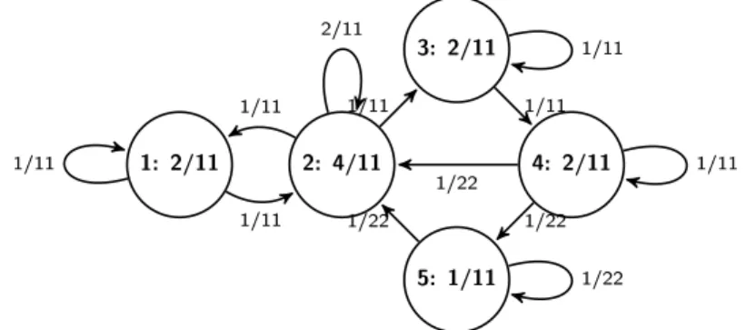
𝑄can also be considered as a p.d. on the state space𝐸∪𝑆, i.e., if we extend the set 𝑉′ of vertices of L(𝐺)as𝑉′ =𝐸∪𝑆, on the line road network. Thus, we can think of𝑄as the distribution of the vehicles on the edges of the road network, see formula (11) in [8]. The distribution𝑄, similarly to traffic trajectories, can also be visualized on the edges, see Fig. 8.
For a positive𝑄on𝐸, let us define 𝜋𝑢:=∑︁
𝑣∈𝑉
𝑞𝑢𝑣 =∑︁
𝑣∈𝑉
𝑞𝑣𝑢, 𝑢∈𝑉, 𝑝𝑢𝑣 :=𝑞𝑢𝑣
𝜋𝑢
, 𝑢, 𝑣∈𝑉.
(5.1)
Note that 𝜋𝑣 >0 for all 𝑣 ∈ 𝑉 by Theorem 3.1. Then, 𝑃 = (𝑝𝑢𝑣) defines a 𝐺- compatible Markov kernel with s.d.𝜋on𝐺. Thus, a Markov traffic defined by the quadruple(𝐺, 𝑃,𝜋, 𝑘)can be introduced by an equivalent way through the triplet (𝐺, 𝑄, 𝑘).
With the help of 2D s.d., we can assign a p.d. to any Markov traffic on the space of traffic configurations which are defined on the edges of the road network.
Namely, let the traffic configurationℎ= (ℎ𝑢𝑣)𝑢⇒𝑣 be a non-negative integer valued function on 𝐸∪𝑆. Here, ℎ𝑢𝑣 denotes the number of vehicles on the edge (𝑢, 𝑣) where𝑢, 𝑣 ∈𝑉 such that𝑢⇒𝑣. We define the two-dimensional distribution𝜎 on the set of traffic configurations ℎwith size 𝑘 (𝑘∈N), i.e., where∑︀
𝑢⇒𝑣ℎ𝑢𝑣 =𝑘. Similarly to (4.1), the two-dimensional distribution𝜎induced by a p.d.𝜋on𝐺as its𝑘-fold convolution has a multinomial distribution with parameter𝑘and𝑄, i.e., for allℎ, we have
𝜎(ℎ) :=𝑘! ∏︁
𝑢⇒𝑣
𝑞ℎ𝑢𝑣𝑢𝑣 ℎ𝑢𝑣!.
In fact, 𝜎 describes the 2D s.d. of a Markov traffic with size 𝑘. One can easily see that the concept of 2D s.d. can also be extended for the second-order Markov traffic.
3: 2/11
2: 4/11
1: 2/11 4: 2/11
5: 1/11 1/11
1/11
1/11 1/11 2/11
1/11 1/11
1/22 1/22
1/11 1/22
1/22
Figure 4. The two-dimensional stationary distribution (on edges) with its equidistributed marginals (on vertices) for the Markov ker- nel in Fig. 1. One can easily check that the sums of probabilities written on the edges in and out each vertex are equal, respectively.
The simulation algorithm presented in this paper is based on the 2D s.d. defined on the road graph. However, it is not an easy task to find a matrix𝑄which satisfies properties (i)-(iii) on a sparse graph. Hence, at first, we propose a method for finding such𝑄which is closest to a given mask matrix𝑀on𝐺in the least square sense. The role of the mask matrix is to specify the weight of edges by modeling the odds of consecutive occurrences of cars on the terminal points of edges in the road network. For example, these weights may stem from observed trajectories for the traffic in a time period.
Let us observe a random sample of trajectories {𝑋𝑖}, 𝑖 = 1, . . . , 𝑘, of size 𝑘 defined by 𝑋1𝑖 ⇒ 𝑋2𝑖 ⇒. . . ⇒ 𝑋𝑛𝑖𝑖, 𝑖 = 1, . . . , 𝑘, where𝑛𝑖 denotes the length of the𝑖th trajectory. The total sample size is given by𝑛:=𝑛1+. . .+𝑛𝑘. Define the total two-dimensional consecutive empirical frequencies as:
𝑛𝑢𝑣 :=
∑︁𝑘 𝑖=1
𝑛∑︁𝑖−1 𝑗=1
𝐼(𝑋𝑗𝑖=𝑢, 𝑋𝑗+1𝑖 =𝑣), (5.2) 𝑢, 𝑣 ∈ 𝑉, where 𝐼 denotes the indicator function. Plainly, 𝑛𝑢𝑣 is the number of consecutive pairs(𝑢, 𝑣)(𝑢, 𝑣∈𝑉) in the trajectories. One can see that the support of the two-dimensional frequency matrix 𝑁 := (𝑛𝑢𝑣)𝑢,𝑣∈𝑉 is a subset of 𝐸∪𝑆.
Clearly,1⊤𝑁1=𝑛−𝑘, where𝑛−𝑘is the corrected sample size. One can also see that the vectors 𝑁⊤1−𝑁1and1are orthogonal. In this case, the matrix𝑁 is a good candidate for the role of the mask matrix𝑀.
We define the optimality criteria for determining𝑄by means of the least squares distance between matrices over 𝐺. Let𝐴= (𝑎𝑢𝑣)𝑢,𝑣∈𝑉 and𝐵 = (𝑏𝑢𝑣)𝑢,𝑣∈𝑉 such that𝑎𝑢𝑣=𝑏𝑢𝑣= 0for all𝑢, 𝑣∈𝑉 where𝑢;𝑣. The least square distance between
𝐴and 𝐵 is defined as
‖𝐴−𝐵‖2𝐺 := ∑︁
𝑢,𝑣:𝑢⇒𝑣
|𝑎𝑢𝑣−𝑏𝑢𝑣|2.
In fact,‖ · ‖𝐺 is the Frobenius norm of the matrices of dimension |𝑉| × |𝑉|which vanish on the entries outside of 𝐸∪𝑆.
To formulate our main result, we need some basic facts on the spectral theory of directed graphs, see [28] for details. The symmetric unnormalized graph Laplacian matrix 𝐿 of a digraph 𝐺 is defined as 𝐿 := 𝐷−𝐴−𝐴⊤, where 𝐴 denotes the adjacency matrix of𝐺and𝐷:= diag{𝑑++𝑑−}.
Theorem 5.1. Let 𝑀 be a non-negative matrix on 𝐺. Then, there is a unique pair(𝑄,κ), where the matrix𝑄on𝐺satisfies properties (i)-(iii) andκ≥0, which minimizes the error function ‖κ𝑄−𝑀‖2𝐺. Moreover, the unique solution to this optimization problem is derived as
κ:=1⊤𝑀1+ (𝑑−−𝑑+)⊤𝜆, 𝑄:=κ−1(𝑀+ (1𝜆⊤−𝜆1⊤)∘𝐴),
where 𝜆 = (𝜆𝑣)𝑣∈𝑉 is called Lagrange vector and defined as a unique solution to the vector linear equation𝐿𝜆= (𝑀−𝑀⊤)1which satisfies the constraint1⊤𝜆= 0 (i.e., ∑︀
𝑣∈𝑉 𝜆𝑣 = 0), and∘denotes the entrywise (Hadamard) product of matrices.
The proof of Theorem 5.1 is based on the Lagrange method, see Appendix in [4]. One can easily see that the error function at the optimum equals to the sum of squared differences (SSD) of the Lagrange vector defined by
SSD:= ∑︁
𝑢→𝑣
(𝜆𝑢−𝜆𝑣)2.
The fundamental statement of Theorem 5.1, as one of the main results of this paper, is that the optimal 2D s.d.𝑄is a low-dimensional perturbation of the mask matrix𝑀. This perturbation term and the normalizing constantκ depend on two components through a unique solution to a vector linear equation. The coefficient matrix of the linear equation is the Laplacian matrix 𝐿 of the road graph which depends only on the graph structure of the road network and independent from the mask matrix. Thus,𝐿can be computed and stored in advance for a given road network. Contrarily, the constant vector of the linear equation depends only on the marginals of the mask matrix, however, it does not depend on its entries and mainly on the road network itself.
After having defined or determined a 2D s.d.𝑄on a road network𝐺, a simple simulation algorithm for generating random trajectories on 𝐺is the following. A trajectory 𝑡 of length ℓ is a generalized path 𝑣0 ⇒ 𝑣1 ⇒ . . . ⇒ 𝑣ℓ−1, 𝑣𝑖 ∈ 𝑉, 𝑖= 0,1, . . . , ℓ−1, which is stored in an ordered list as𝑡= [𝑣0, 𝑣1, . . . , 𝑣ℓ−1]. Note that𝑣𝑖=𝑣𝑖+1 is also allowed for any index𝑖, i.e., a vehicle may stay in place after a timestep. The temporary set of generated trajectories is stored in a dictionary𝐷
which consists of key-value pairs(𝑣, 𝑇𝑣). Here, the key𝑣∈𝑉 identifies a node in the road graph, and the value𝑇𝑣 = [𝑡0, 𝑡1, . . . , 𝑡𝑛𝑣−1] is an ordered list of trajectories 𝑡𝑗,𝑗= 0,1, . . . , 𝑛𝑣−1, of length𝑛𝑣 such that the last element of all trajectories in 𝑇𝑣 is𝑣, i.e., the trajectories end at the node𝑣. In fact,𝑇𝑣 is a list of lists for each 𝑣∈𝑉. Let𝑇 denote the final set of trajectories as the output of the algorithm. By generating random pairs (𝑢, 𝑣) from 𝑄 successively, 𝐷 is updated, and then𝑇 is derived in the following way. If𝑇𝑢is not empty, then let the trajectory𝑡be given by appending𝑣to the first trajectory in𝑇𝑢. Moreover, let us delete this trajectory from the list𝑇𝑢. If the length of𝑡is large enough, then let us add it to𝑇, otherwise add it to the list𝑇𝑣. If𝑇𝑢was empty then append the list [𝑢, 𝑣]to𝑇𝑣.
Algorithm 1:Trajectory simulation.
Input: 𝑄: two-dimensional stationary distribution 𝑚: maximum trajectory length
𝑛: number of simulated consecutive pairs Output: T: list of trajectories
/* initialization */
𝐷={}; /* temporary dictionary */
𝑇 = [ ];
/* iterating over simulated pairs */
for𝑖= 1 to𝑛do
pick a random pair(𝑢, 𝑣)∼𝑄;
if 𝐷[𝑢]is not empty then
𝑡=𝐷[𝑢][0]; /* temporary trajectory */
append node𝑣to 𝑡;
delete the first element of𝐷[𝑢];
else
𝑡= [𝑢, 𝑣];
endif length(𝑡) =𝑚then append𝑡 to𝑇; elseif 𝑣∈𝐷 then
append𝑡to𝐷[𝑣];
elseappend(𝑣, 𝑡)to𝐷;
end end end
/* appending the trajectories in temporary dictionary to the output for*/𝑣 in𝐷 do
append𝐷[𝑣]to 𝑇;
end
Having finished the random generation of pairs, let us append the trajectories of whole𝐷to the final set𝑇. One can easily see that the longer trajectories are at the head of𝑇. A pythonic pseudo-code of the above procedure is in Algorithm 1. After the simulation, the generated trajectories can be visualized by using a digital map system, e.g., Google Maps or OpenStreetMap. Finally, we note that, in a typical step of the algorithm, a trajectory moves from the first position of a trajectory list to the last position of an other one. This is a kind of mixing which helps to avoid the formation of very unbalanced trajectories.
6. Results
In our work, OpenStreetMap (OSM) was used which is a community project to build a free map of the world. OSM data is available under the Open Data Com- mons Open Database License (ODbL). The representation and storing of map data is based on only three modeling primitives: nodes, ways, and relations.4 A node represents a geographical entity with GPS coordinates. A way is an ordered list of at least two nodes. A relation is an ordered list of nodes, ways, and/or relations.
Users can export map data at the OSM web site manually, selecting a rectangular region of the map. OSM uses OSM XML and PBF formats for exporting map data. Software libraries for parsing and working with OSM data are available for several programming languages.5
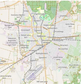
We started our processing by building a graph from the OSM map of Debrecen in the bounding box defined by the coordinates N47.4771, W21.5565, N47.571, W21.6918, see Fig. 5. Because we only need those nodes that can be reached by vehicles, we had to filter the OSM file and collect only specific types of way nodes.
In the OSM file, a way is a sequence of OSM nodes, so naturally, the nodes of ways become nodes in the graph. For every node we store the node’s OSM ID and its coordinates. We also insert an edge into the graph to connect each pair of nodes that follow each other in a way. We used the PyOsmium library for processing the OSM files and the NetworkX Python library for building the graph. The result of this processing is an aperiodic strongly connected road network of Debrecen augmented by the ideal vertex 0. The descriptive statistics of edges of the road graph are: Min=0.3395, Q1=10.7906, Med=24.7830, Mean=49.9052, Q3=67.6021, Max=1167.4902 (in meters). The degree distributions of this road network are visualized in Fig. 6.
To evaluate the performance of the proposed algorithm a simple simulation study was conducted at different sample sizes for the road network of Debrecen.
In the simulations, we kept the length of trajectories low and the number of tra- jectories high compared to the size of the road network. By our experience, the real traffic trajectories posses these properties. All simulations were carried out in Python. The codes and datasets of our simulation are available upon request.
We have also implemented the model in the OOCWC system. Regarding RCE,
4http://wiki.openstreetmap.org/wiki/Elements
5https://wiki.openstreetmap.org/wiki/Frameworks
we have performed several modifications. First, we extended the operation of RCE to be able to handle kernel files for transition probability matrices and 2D stationary distributions, respectively. These kernel files can be loaded to the RCE software, so all nodes of the simulation graph will have the corresponding transition probability vector from the Markov kernel file. For this, we had to extend the shared memory segment of RCE.
Debrecen Debreceni
Regionális és Innovációs
Ipari Park
száros Gergely- kert
Tócóvölgyi lakótelep
Wesselényi- lakótelep Domokos Márton-
kert
József Attila- telep Nyugati Ipari
Park
Biczó István- kert Hatvan utcai
kert Liget II lakópark
y Mihály- kert
Veres Péter- kert
Boldogfalvikert
Déli ipari park Széchenyikert
Egyetemváros
Nagyerdőalja
Bozzaytelep Kincseshegy
Műhelytelep Sámsonikert
Biharikert Dobozikert
Júliatelep
Köntöskert
Lencztelep Pércsikert
Tégláskert Epreskert
Repülőtér Sestakert
Vargakert Ispotály Libakert Úrrétje
Pac
354 471
35
47
4 4
4808
4814 Vámospércsi út
Mik Nyíl utca
Kassai út
Vágóhíd utca
Diószegi út Acsádi út
Kamarás- halom 121 m
Basa-halom 116 m
Terület
Debrecen nemzetközi repülőtér
Figure 5. The map of the observed area. The graph created from the OSM data has 14,465 nodes, 29,770 edges, and covers a total of
799.4 km of road. The size of the area is about 106 km2.
© OpenStreetMap contributors.
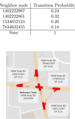
For a visual explanation of the transition probability vector, see Fig. 7. We are at the graph vertex (or intersection) of OSM node ID 26755459 (with GPS coordinates 47.5417164, 21.6097831). From this node, we can move towards nodes 1402222987, 1402222861, 1534652124, and 7834632455. The transition to each node has a certain probability, see Table 2.
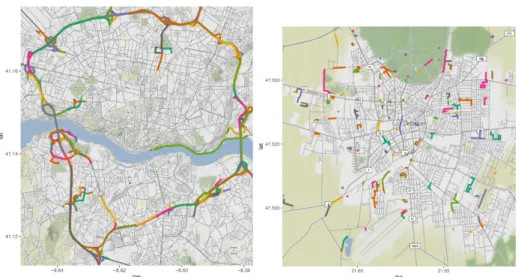
We generated trajectories using Algorithm 1. For this, we created a𝑄for Deb- recen, but since we have no real-world traffic data, we generated random values for the 2D stationary distribution. To compare our results, we generated trajectories using the same algorithm for Porto, Portugal. In case of Porto, we could calculate a 𝑄that is approximated based on real-world data, namely, the Taxi Trajectory Prediction dataset, following the methods described in paper [4]. One can easily see on Fig. 8 that the trajectories generated based on a real𝑄have more realistic shapes (in case of Porto, see the left subfigure in Fig. 8), while the others are quite random (in case of Debrecen, see the right subfigure in Fig. 8b). An interesting question arises: can we tell if a 𝑄 reflects the real traffic system of a city? We assume that a 𝑄 can be validated with trajectories generated from it. If these trajectories reflect the real traffic in a certain level, we can accept 𝑄. Elaborating
this validation technique is one of our future work.
4 2913
8162
3011
375 0
2000 4000 6000 8000
0 1 2 3 4
indegree
count
5 2913
8151
3029
367 0
2000 4000 6000 8000
0 1 2 3 4
outdegree
count
4 3019
16504
8790
1453
0 0
0 5000 10000 15000
0 2 4 6
indegree
count
5 3020
16474
8843
1428
0 0
0 5000 10000 15000
0 2 4 6
outdegree
count
Figure 6. The degree distribution (first: in-vertices, second: out- vertices, third: in-edges, fourth: out-edges) histograms of the
Debrecen map road graph.
Table 2. Transitions of intersection 26755459.
Neighbor node Transition Probability
1402222987 0.24
1402222861 0.32
1534652124 0.26
7834632455 0.18
Sum 1
Figure 7. A visual explanation of transitions of intersection 26755459. TP means transition probability, nodes are highlighted with red. Base map and data from OpenStreetMap and Open- StreetMap Foundation. © OpenStreetMap contributors. Anno-
tated by the authors.
Figure 8. Generated trajectories in Porto (left: 𝑛= 200,000,000;
𝑚= 75) and Debrecen (right: 𝑛= 50,000,000;𝑚= 35) simulated with Algorithm 1.
7. Conclusions
In this paper we have described various graph models for proper road networks and introduced the concept of Markov traffic. By tools of Markov chain theory, we have proven the existence and uniqueness of a stationary distribution for any Markov traffic on strongly connected and aperiodic road networks. We have also derived an explicit formula for the stationary distribution and the two-dimensional stationary distribution. Finally, we have proposed a simulation algorithm for generating ran- dom trajectories which follows the two-dimensional stationary distribution which being closest to a given mask matrix on the road network.
To test our theories, we have implemented the proposed model in our simulation program (RCE) using OpenStreetMap. The whole project (including RCE) is available for download.6
Future work will focus on the further improvements and the possible applica- tions of our simulation algorithms, e.g., modelling the pollution or energy consump- tion in Smart Cities.
Acknowledgements. The authors would like to thank all actual and former members of the Smart City group of the University of Debrecen. We are especially grateful to all of the participants of the OOCWC competitions and the students of the BSc courses of “High Level Programming Languages” at the University of Debrecen.
6https://github.com/rbesenczi/Crowd-sourced-Traffic-Simulator/blob/master/
justine/install.txt