THE ATMOSPHERE* TRANSMISSION OF RADIATION THROUGH

Chapter 5

TRANSMISSION OF RADIATION T H R O U G H T H E ATMOSPHERE*

T h e treatment of transmission of radiation through the atmosphere of the earth begins customarily with a study of the spectroscopic properties of atmospheric constituents, and is then followed by a discussion of fluxes, heating rates, and radiative transfer in real atmospheres.These topics are generally associated with meteorological research; Goody has written a definitive text on the subject.¹ In the following discussion, we present a brief survey of representative problems and note that analytical techniques, similar to those used in Chapter 1 for the theoretical calcula- tion of gas emissivities, are employed in estimating radiant-energy transmission through the atmosphere.

5-1 C o m p o s i t i o n of the a t m o s p h e r e

Our knowledge of atmospheric composition is largely based on observations of solar radiation at various altitudes.^{2 - 1 2} T h e observed intensity in the solar spectrum decreases rapidly in the far ultraviolet region of the spectrum because of energy absorption high in the atmos- phere where photoionization and photodissociation of molecules occur.¹'^{1 3 - 2 2} I n the upper atmosphere, the collision frequency is too low to maintain a Boltzmann population of molecular vibrational states. As a consequence, nonequilibrium effects are important and the kinetic temperatures tend to be quite high (1000 to 1600°K for the earth).

Figure 5-1.1 shows the temperature distribution as a function of height in the atmosphere; the Nicolet nomenclature,¹⁴ which describes the gross characteristics of regions of the atmosphere, is also indicated. T h e atmosphere is assumed to have a constant adiabatic lapse rate (i.e., a

* Section 5-2 is by S. S. PENNER and D. B. OLFE; Sections 5-1 and 5-3 to 5-5 are by L. D. GRAY.

231

232 5. ATMOSPHERIC TRANSMISSION

constant rate of decrease of temperature with height) in the troposphere, where convection is the primary mode of heat transfer. In the tropopause, and above, heat transfer occurs mainly by radiation. For an atmosphere in radiative equilibrium, the temperature should remain relatively independent of height,¹ as in the tropopause. The rise in temperature in

160

woh

120

»oh ί eoh

60

40

20

01

1 1 IONOSPHERE

O g - ^ O + O

OZONE LAYER

CHEMOSPHERE MESOPAUSE MESOSPHERE STRATOPAUSE STRATOSPHERE TROPOPAUSE TROPOSPHERE 150 200 250 300 350 400 J L

TEMPERATURE, °K

450 500 HO0002 J Q 0 0 I 6 -m.oi HQ06

^Q25

Joe

I² I^{1 2} -155 -|265

JlOI3 E ιυ"

cr

ÜJ

£

FIG. 5-1.1. Temperature distribution as a function of height in the atmosphere of the earth.

the stratosphere is associated with the formation of the ozone layer.

Absorption of ultraviolet radiation in the regions of the Schumann- Runge continuum (λ < 1760 Â) and Herzberg bands (λ < 2420 Â) leads to dissociation of 02 . Ozone is subsequently formed by the reaction O + 02 + M - > 03 + My where M is any third body. Below about 40 km, this reaction is so rapid that most of the oxygen atoms produced by the dissociation of 02 form 03 molecules. T h e ozone layer has a maximum concentration near 30 km with most of the 03 occurring between 10 and 40 km. Although the total amount of ozone in the atmosphere is small (about 0.3 cm-atm), it greatly affects the atmospheric heat balance and is responsible for the short-wavelength cutoff of the solar spectrum in the continuum of the Hartley bands.

T h e second temperature rise in the atmosphere occurs above 90 km

CH CO HI No ΝΠ NI ΟΠ 0 1 OH

N?

NO

<*

05

N2

O2

l·- [- k L- u

| ION

ION T

La X

ION J

H Γ

CAMERON

«Afty

HARTLEY

COMET 1

XX

X X

r

HUGGINS VEGARD-KAPLAN 2+

SCHUMANN

-J L

1 Γ

ß X

X X X

X

Γ 0 X

X

XX

CHAPPUIS

-RUNGE HERZBERG

1 1 1

"Ί 1 1 1 1—

X

MEINEL VIBRATION-ROTATION

MEINEL

1 + ATMOSPHERIC

...1 __L_ .._l 1 1

r~ 1

-J -J -J

^ -J J

^

1 - 1

0 1000 2000 3000 4 0 0 0 5000 6000 7000 8000 9000 lOpOO 11,000 12,000 13,000 WAVELENGTH, A

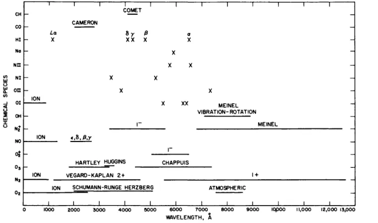
FIG. 5-1.2. Location of spectral lines and bands that have been observed in absorption or in emission by the atmosphere of the earth, in the visible and ultraviolet regions of the spectrum.

o o S o CO

3

o Ml H X w o

ιη *j X m

234 5 . ATMOSPHERIC TRANSMISSION

where dissociation of oxygen takes place. T h e chemosphere is the region of the atmosphere where chemical reactions occur (e.g., dissociation and recombination),²³ while such processes as 02 -f- hv -> O£ + e~ are observed in the ionosphere. Solar radiation with wavelengths less than about 1000 Â causes the formation of ions from atmospheric constituents.

Figure 5-1.2 shows the location of various bands which absorb the incoming solar radiation in the visible and ultraviolet regions of the spectrum. Figure 5-1.2 also shows the positions of lines and bands which have been observed in emission. Emission of light in the upper atmos- phere is associated with the occurrence of such interesting phenomena as the aurora borealis and airglow and involves recombination reactions for atoms and ions, collisions with incoming solar particles, and various photochemical reactions.^24-94

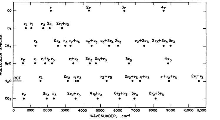
T h e atmosphere is nearly transparent between 0.3 and 0.8 /x, except for absorption produced by telluric counterparts of Fraunhofer lines and the following weak bands: the Huggins bands of 03 (0.3 to 0.35 /x), the Chappuis bands of 03 (0.5 to 0.7 /x), and the atmospheric bands of 02 (0.69 and 0.76 μ,). The infrared spectrum, beyond about 0.8 μ,, contains a large number of vibration-rotation bands attributed to the minor constituents of the atmosphere: C 02, H20 , CH4 , CO, N20 , and 03 . Figure 5-1.3 shows the location of some of the band centers for these minor constituents. The two major constituents of the atmosphere, 02 and N2, are homonuclear diatomic molecules without permanent or oscillating dipole moment, and hence do not exhibit vibration-rotation bands.

With the exception of water vapor and ozone, the minor constituents appear to be uniformly distributed throughout the atmosphere. Most of the water vapor absorption takes place near the ground, but it is highly variable because the humidity of the air fluctuates widely with geography, season, and time of day. Dust, haze, and clouds absorb strongly in the infrared and are mainly responsible for light scattering in the visible regions of the spectrum. The concentration of dust and haze is variable, but generally decreases rapidly with height. The particle sizes depend on the relative humidity; the concentration of particles in the air is smallest when the relative humidity is low. Allen¹⁵ has listed extinction coefficients for molecular scattering and absorption by dust for the spectral region from 0.20 to 4μ,.* A very considerable amount of basic work has been done on the absorptive properties of the atmospheric constituents in the infrared.^95-170

* For a detailed discussion of light scattering, reference should be made to Chapter 4.

CO

Os

Lü O CL C H4

OC

<

O N20

1· 1

tu -1 O 2

H20

C02

U

—

*2

•

•

ROT

"2

• Ί —

y\

•

v4

•

•

J

1 y

•

1/3 2i/, 2i/

• ·

2* 4

•

• ·

*2

•

3" 3 * 3

• · l

"Ί 1

,+*2

•

"3 "2+"4

• ·

•

2i/2 ^1/3

• · · 2*2+1/3

•

- J 1 1 2i/

•

• ·

2"3 ^ Ι + ^

• · 1/2+1/3

•

4i,2+*3

• 1

- 1 1 ι 1 3v 4i/

• ·

2v3 V2+21/3 2i/3-r-2i/4 3i/3

• · · ·

31/3 4 v3

• · 2^+1/3 ν,+1/3 Ί + ^ + ^

• · · 61/2+1/3 31/3 21/2+31/3

• · · _ l 1 1 1

"Ί

1

_J

2".⁺»5

• -J

_J

o o

o

O O

M

o

CD

8 M

0 1000 2000 3000 4 0 0 0 5000 6 0 0 0 7 0 0 0 8000 9 0 0 0 ΙθρθΟ lipOO WAVENUMBER, cnrH

FIG. 5-1.3. Location of vibration-rotation bands for the minor constituents in the atmosphere of the earth.

to

236 5. ATMOSPHERIC TRANSMISSION

5-2 Spectral t r a n s m i s s i o n through the a t m o s p h e r e at 10,468 A *

Radiant-energy absorption at a frequency that is well separated from spectral lines belonging to atomic or molecular emitters is of particular interest with regard to the attenuation of laser beams passing through the atmosphere. As an interesting example, we consider a narrow line centered at 10,468 Â and we use approximate equivalent widths for the known spectral lines as listed by Babcock and Moore.² It is found that, if Lorentz line contours are assumed, the greatest contribution to the absorption at 10,468 Â appears to come from the 1.1-/x water vapor band, which gives a spectral absorptivity of about 3 X 10^{- 5}, or an absorption coefficient of 1.5 X 10^{- 1 1} c m^{- 1} for a 45° path (for an atmosphere extending two scale heights with a pressure of \ atm).

T h e Lorentz line contour is given by

C L·

(5-2.1) π (ω — ω0)² + b² '

where Ρω is the spectral absorption coefficient (cm^_1-atm^_1), S is the line integrated intensity (cm~²-atm^_1), ω is the wavenumber (cm^{- 1}), and b is the half-width (cm^{- 1}), i.e., half the line width at half the peak absorption coefficient. If the line is so weak that there is little absorption at the line center (SX < Ab), then the equivalent line width W may be estimated from the following relation:

W = [1 -exp(-P^/»CO wX)]dw~SX. (5-2.2)

Here X is the optical depth, which is defined as the beam length multi- plied by the partial pressure of the absorbing species. For strong lines (SX > 4è),

W~2(SbXfl2. (5-2.3

) In the line wings, where the spectral absorption Αω is small,

π(ω — ωWb 0)²

and

for W < 4b (5-2.4)

1 / W \²

Αω~-±-(—-—) for W>4b. (5-2.5)

This section is based on unpublished studies performed by Penner and Olfe.^170a

5-2 SPECTRAL TRANSMISSION THROUGH THE ATMOSPHERE 237

The contribution to the absorption Αω from the lines between ωλ and o>2

(with ωχ and ω2 both located at either higher or lower frequencies than ω) may be estimated by distributing the line intensities uniformly between ω1 and ω2 . The following expressions are obtained in this manner: _

Αω~—7 ^ - r- for W<4b (5-2.6)

π(ω — ωλ) (ω — ω2)

and

NW² —

Λ , ^ Ί Γ Τ ^τι Γ ^{f o r} W>4b, (5-2.7)

4π(ω — ωλ) [ω — ω2)

where Ν is the number of lines and W the mean equivalent width.

The computed line widths⁹⁸ (line width y = 2bjp) for the v2 and 2v2

vibration-rotation bands and for the pure rotation spectrum generally lie in the range 0.05 to 0.11 cm^{_ 1}-atm^{_ 1}. Assuming an average pressure of \ atm, the half-width b for all of the water vapor lines is taken as 0.02 cm"¹.

In order to carry out the calculation of atmospheric absorption at 10,468 Â, it is convenient to divide the spectral lines into several groups.

First, the lines identified in Babcock and Moore² as being atmospheric (but not 02 lines) and centered around 10,468 Â in a 600-Â region are sufficiently weak to allow the use of Eq. (5-2.4) (the half-width for H20 is used since nearly all of these lines belong to H20 ) . T h e total contribu- tion from these lines, of which there are 24, is 4 - 2 x 10^{- 7} at 10,468 Â. Using Eq. (5-2.4) to estimate the contribution from the 23 lines in the 02 band, which extends from 10,584 to 10,719 Â, yields Αω ~ 1 x 10^{- 7}. The half-width for 02 has been assumed to be the same as that for H20 ; however, this is not a critical assumption since the 02 contribution to the absorption is about two orders of magnitude less than the contribution from the strong H20 lines. The absorption from the weak atmospheric lines between 10,768 and 12,468 Â may be computed from Eq. (5-2.6) by dividing the region into 6 groups of about

100 lines each. This procedure yields a contribution of Αω c^ 5 X 10^{- 7}. The contribution from the 114 strong atmospheric lines between 11,103 and 11,601 Â is approximately J w ^ 3 x 10^{- 5}, as computed from Eq. (5-2.7). It should be noted that the widths of the strong lines given in Babcock and Moore² are only "eye estimates,^,, and thus only approximately equal to the " t r u e " equivalent widths. Hundreds of very weak atmospheric lines have been omitted from the table of Babcock and Moore.² However, the preceding calculations indicate that only the strong lines make important contributions if collision broadening follows a Lorentz contour.

238 5 . ATMOSPHERIC TRANSMISSION

The table of Babcock and Moore² contains a number of unidentified lines, which may be either of solar or of atmospheric origin. There exists one such line at 10,465 Â, which will contribute an absorption Αω ~ 2 X 10^{- 5} if it is an atmospheric line. The other 41 unidentified lines in a 300-Â region near 10,468 Â will contribute 4 - 5 x 10~⁶ if they are all atmospheric lines. Thus the contribution of all uniden- tified lines will not be of a greater order of magnitude than the value Αω ~ 3 X 10^{- 5} computed for the strong H20 lines.

In order to express the absorption in terms of an absorption coefficient, we consider the atmosphere to be at a pressure of \ atm and to extend two scale heights (about 50,000 ft) above sea level. The length of a path at 45° to the horizontal is approximately 2 X 10⁶ cm. Therefore, an absorptivity of 3 X 10~⁵ corresponds to an absorption coefficient Κ = ΡωΡπ2ο= 1-5 X 10-¹¹ cm-*.

The equivalent line widths W for the strong lines of the 1.1-/x H20 band given in Babcock and Moore² are only approximately correct. It is, therefore, interesting to verify the estimated order of magnitude by comparison with the integrated band intensity a. Since most of the important lines in the band are strong, the following approximate relation holds:

oc ~ NW²/4bX. (5-2.8)

The optical depth X for H20 can be related to the length L (cm) of precipitable water vapor in a vertical column through the expression

The factor sin 45° appears because the observations of Babcock and Moore² were made at an angle of 45° with respect to the horizontal.

Using the approximate value a ~ 0.3 cm~²-atm^_1, and the values N and W determined from Babcock and Moore,² we obtain L ^ 4 cm, which is a reasonable order of magnitude for the amount of precipitable water vapor in the atmosphere.

Undoubtedly the greatest error in the calculation of the absorption at 10,468 Â arises from our use of the Lorentz line contour at very large wavelength distances from the line centers. In computing the contribu- tion from the l.l-/x water vapor band, distances of 635 to 1133 Â from the line centers were considered. Measurements in the near wings of lines have yielded values a factor of 2 or so above the Lorentz value. For this reason, it is not unreasonable to believe that the contours will be appreciably below the Lorentz values at very great distances from the

5-3 TRANSMISSION ALONG A SLANT PATH 239

line centers. T h e problem of spectral line shape in the far wings is an important problem which requires further study.

T h e contributions from the lines considered in the preceding dis- cussion are actually of minor importance in determining the value of the linear absorption coefficient at 10,468 Â. This conclusion follows from observations¹⁷¹ of solar attenuation along long slant paths which indicate the presence of a broad absorption line centered at 10,608 Â. This line has since been identified as belonging to a very short-lived (lifetime

~ 10~ⁿ sec) oxygen dimer, ( 02)2, in which forbidden molecular transitions are momentarily allowed during the lifetime of the dimer.

The absorption due to the dimer has also been estimated in laboratory studies¹⁷¹'¹⁷² by using very long absorption paths. At the line center (10,608 Â), the broad line contributes a value of 1.5 X 10~⁸ c m^{- 1}; at 10,468 Â, the absorption coefficient has fallen to 1.5 X 10~⁹ c m^{- 1}, i.e., it is about two orders of magnitude larger than our estimate for the linear absorption coefficient produced by all of the Lorentz line tails associated with all of the identified lines in the Babcock and Moore atlas.²

T h e extent to which dimerization of other atmospheric constituents ( N2, H20 , C 02) dominates transmission of radiation in selected spectral regions clearly requires further study.

Atmospheric transmission of laser radiation has been considered recently by Plass from a rather different point of view.¹⁷³ T h u s Plass first develops a simple procedure for estimating the transmittance when absorption occurs by an isolated spectral line and then considers many lines in an Elsasser band model (i.e., equally intense, equally spaced spectral lines).¹⁷³

5-3 T r a n s m i s s i o n along a slant path through the a t m o s p h e r e

Transmission of radiation through a real atmosphere depends on the types and number density of molecules present and on the ambient pressure and temperature. In general, these quantities vary continuously along a slant path through the atmosphere, and a great deal of effort^174-204'* has gone into developing approximations which reduce the problem to one of computing the transmission of an equivalent homoge- neous 'average'' atmospheric path. Plass¹⁸⁰ has given a summary of useful approximations for various band models. While it is possible, in prin-

* This section is largely based on a paper by Gray and McClatchey.

240 5. ATMOSPHERIC TRANSMISSION

ciple, to calculate atmospheric transmission by considering individual lines separately,²⁰⁴ it is evident from the discussion given in Section 5-2 that such a procedure is extremely laborious and impossible to implement with great assurance for success. The use of approximate methods^196-203 is clearly desirable for reducing the computation time and for the calculation of spectral transmission in agreement with low-resolution measurements.

Linear molecules, such as CO, C 02, and N20 , have vibration- rotation bands in which the line intensities and the spacing between the lines vary regularly as a function of frequency. Figure 5-3.1 shows the

z o

CO CO

5 CO

z <

cr 1-

01 0.2 [ 0.4 L 0.61 0.8 h 1.0 Γ

2000 2050 2100 2150 2200 2250 WAVENUMBER, cm^-1

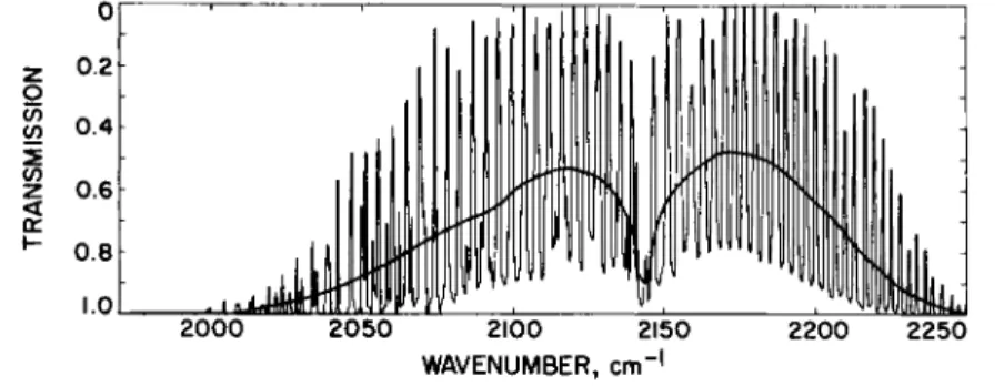
FIG. 5-3.1. Transmission of carbon monoxide; reproduced from Gray and McClatchey.¹⁸²

spectra of the 0-1 bands of CO; the weak lines are due to isotopic CO and to the "hot" bands, i.e., the 1-2, 2-3, etc. vibrational transitions which also absorb in the 4.7-μ, region. The random-Elsasser band model¹⁹⁷ is particularly useful for estimating transmission in such regular bands; representative results obtained in calculations of this type, which yield the average transmission for a spectral interval equal to the line spacing, are shown in Fig. 5-3.1.

Molecules such as H20 , 03, and CH4, which are not linear, exhibit a much more irregular distribution in the intensities and spacings of the rotational lines within a band; for these spectra, the statistical band model (cf. Section 1-6D) is especially suitable in transmission calcula- tions.¹ In the following discussion, we shall consider only linear mole- cules.

In order to estimate the accuracy with which the transmission can be computed for a nonhomogeneous path through the atmosphere, we have made numerous comparisons of results computed by using the random-Elsasser band model with laboratory measurements of homo- geneous-path transmission. In this model, it is assumed that a given

5-3 TRANSMISSION ALONG A SLANT PATH 241 vibration-rotation band may be divided into a number of spectral intervals such that the absorption due to the rotational lines in any particular interval is represented by the absorption of an Elsasser band.¹⁹⁶ An Elsasser band consists of equally spaced, equally intense spectral lines. Clearly, if the width of the spectral interval is small compared with the width of the entire band, but sufficiently large to contain several lines, then the intensity and spacing of the rotational lines within the interval will be well approximated by the intensity and spacing of a line located at the center of the interval (unless the center of the interval coincides with the band center, in which case the calcu- lated average intensity is incorrect). Since the various vibration-rotation bands contributing to the total absorption at the wavenumber ω are randomly located with respect to one another, the spectral transmission τ(ω) is given by the product of the transmissions¹⁹⁷ due to the Elsasser bands corresponding to the various individual vibrational transitions, viz.,

τ(ω) = Π*<Η> (5-3.1)

i=l

where N is the total number of vibrational transitions. The average transmission of an Elsasser band is given by¹⁹⁶

/./to/sinh ß

T = 1 _ sinh ß I0(u) [ e x p ( - u cosh ß)] du, (5-3.2) where ß = l-rrb/d, x = SX\2-nby and I0(u) is the Bessel function of imaginary argument and order zero. Here b is the half-width, S is the line intensity, d is the line spacing, and X is the optical depth. Equation (5-3.2) may be rewritten in terms of the tabulated²⁰⁵'²⁰⁶ Schwarz function Ie(ky z) as

T = 1 — tanh ß [7e(sech ß, ßx coth ß)], (5-3.3) where

Ie(k, z) = f I0(ku) e~^u du. (5-3.4)

J o

In our calculations, we have utilized a computer subroutine (due to L. D. Kaplan and A. R. Curtis) in which the transmission from the asymptotic expansion²⁰⁵ for Ie(k, z) is calculated, i.e., the following approximation is used:

00 / k \²ⁿ /2n\ r ^{2 n} ?^l l

' * ' > - £ £ ) (?)['—Σ^]- (».5»

242 5 . ATMOSPHERIC TRANSMISSION

Hence it follows that

t. o £ / ^{s e c h} ß \²ⁿ l²ⁿ\

x j l - e x p [ ( - ^ c o t h Ä | - ^ L ^ ] j . (5-3.6) T h e local values of ß and x are estimated by assuming that they vary continuously as a function of rotational quantum number m. T h e usual expression for the positions of the rotational lines in the P- and R- branches of a band, for a linear molecule, is*

«,(«) = %, + (^B'i + B"ù^m + (^B'i - ^Bd ^m* - m + D't) m». (5-3.7) Here œoi is the band origin of the ith vibration-rotation band; B is the rotational constant; D is the centrifugal stretching constant; m is related to the rotational quantum number as follows: m = — J" for the P-branch and m = J" + 1 for the i?-branch; double primes identify the lower vibrational state and single primes the upper vibrational state. T h e values of m corresponding to the location of an actual spectral line are, of course, integers. In the random-Elsasser model, the band is broken up into a number of small intervals; Eq. (5-3.7) is then used to obtain the value of m corresponding to a line located at the center of the interval for each vibrational transition. T h e m-values obtained in this manner are, in general, nonintegral. Using the m-value obtained from Eq. (5-3.7), the local rotational line spacing becomes

d.(m) = (B» + B'.) + 2(B'. - B\) m - 6(ZX + D») m\ (5-3.8) Similarly, the rotational energy of the lower vibrational state is found from the expression

ωτ(τη)" = B".m{m - 1) - ZX'm²(m - l)². (5-3.9) The local rotational line intensity is finally obtained from the relation⁺

SAm)

^ ( Ä f r f K (- %)\ [. - exp (- *$*-)] .

(5-3.10)

* See Eq. (Ill, 139) of Herzberg²⁰⁷ and Eq. (IV, 21) of Herzberg.²⁰⁸ t See Eq. (7-115) of Penner.²⁰⁹

5-3 TRANSMISSION ALONG A SLANT PATH 243 Here N is the total number of molecules per unit volume per unit pressure, g" is the degeneracy of the lower state, h is Planck's constant, k is the Boltzmann constant, c is the velocity of light, T is the absolute temperature, μί is the dipole matrix element for the fth vibrational transition, QY is the vibrational partition function, QT is the rotational partition function, ω" refers to the lower state (ω" = ω'ί -f ωγ , where the subscripts r and v refer to rotation and vibration, respectively), and R%/?}'m> is the rotational matrix element. For parallel bands (A I = 0) of linear polyatomic molecules (e.g., C 02, N20 ) , the square of the rotational matrix element is*

( ^ 4 0² = ^ ^ (5-3.11)

for the P - and P-branches. For the diatomic molecule CO, there is no angular momentum associated with vibration, and the rotational matrix element is the same as for a Σ —► Σ(1 = 0—> I = 0) transition of a linear polyatomic molecule. The contributions of Q-branches are not well approximated by the random-Elsasser model and are treated separately, as will be discussed later on. For perpendicular bands with AI = -f 1, the square of the rotational matrix element for the P - and P-branches is given by⁺

with Al = — 1 , it is

\*<m"^m' ) — φ ^ · (5-3.13)

For unsymmetrical molecules such as CO, NNO, and ^{1 2}C^{1 8}0^{1 6}0, all of the lines appear in the spectrum and the intensity and line spacing, as given by Eqs. (5-3.10) and (5-3.8), respectively, are used in computing the local value of the transmission. However, for symmetrical molecules such as ^{1 2}C^{1 6}02 and ^{1 3}C^{1 6}02, alternate lines are missing for 27 —► 27, Σ —► Π and Π —> Σ transitions, and both the line intensity and line spacing are doubled. The /-doubling of the Π -> 77, A —> A, etc. transi- tions was not included in the present calculations; instead, a simple average value was used for B and D in Eq. (5-3.7) for the line positions.

In transitions for which the vibrational matrix element had not been measured directly, the harmonic oscillator approximation was used. The

* See Eq. (IV, 81) of Herzberg.²⁰⁷

t See Eqs. (IV, 82) and (IV, 83) of Herzberg.²⁰⁷

244 5. ATMOSPHERIC TRANSMISSION

spectroscopic constants, Bv and DY , have been given by Courtoy¹²¹'¹²² for C 02, by Tidwell et a/.¹⁶⁰ for N20 , and by Benedict et a/.¹⁴⁵ for CO.

The rotational lines have been assumed to be broadened only by colli- sions and the half-width of the lines was taken to vary as ^ Γ^{- 1}/², where p is the effective pressure, i.e., p = ΣρίΒί where pi is the partial pressure of the îth chemical species and Bi is the relative broadening ability of that species.¹³⁷ In the calculations, the following values of the half-width for nitrogen broadening were used at 300°K and a pressure of 1 atm:

carbon dioxide,²¹⁰ b = 0.07 c m^{- 1}; carbon monoxide,¹⁴⁴ b = 0.07 c m^{- 1}; nitrous oxide,¹⁶⁶ b = 0.05 c m^{- 1}. All of the isotopic species with a relative abundance greater than 5 X 1 0^{- 6} were included. T h e measured band intensities summarized in Appendix 5-1 were employed.

For perpendicular bands, the ^-branch has about half of the total integrated intensity of the band. Because the lines in this branch are closely spaced, the £)-branch contributes much less than half of the total band absorption. These branches have been treated separately in computing the transmission. T h e actual line positions were found from the expression

«,(/) = ω0 + (B'y - B;) JU + i) - ( D ; - D;) J\J + i)²; (5-3.14) the line intensities were calculated from Eq. (5-3.10) by using the rotational matrix elements

(Rr-*r ) = 4/"(/" + 1) ' (5-3.15) The absorption coefficients for all of the lines in the ^-branch were summed at intervals of 0.01 c m^{- 1} throughout the branch, and the transmission was then computed from the relation

r„ = e x p ( - PJO = exp ( - ^ Ç ( ω _ ^ , + „ ) . (5-3.16) The equivalent widths of Q-branch lines were computed by numerical integration. Because the random-Elsasser band model yields an average transmission for a spectral interval equal to the line spacing dy it was assumed that the average transmission for the ^-branch* is given by the expression

TQ = \-[WQI(B" + B')]; (5-3.17)

* The width of the Q-branch is generally greater than d and Eq. (5-3.17) refers to the fraction of the total equivalent width that occurs in an interval of width d.

5 - 3 TRANSMISSION ALONG A SLANT PATH 245 this procedure yields comparable resolution for the P-, Q-> and R- branches. A similar procedure is necessary to obtain the line-wing emission beyond the bandheads, but was not included in the completed calculations. The weak g-branches of the parallel bands were not included in the calculations.¹²⁰

Figures 5-3.2 through 5-3.7 show both computed transmission spectra and laboratory measurements on homogeneous paths for various gases.

In a first approximation to the transmission through the atmosphere, the real, nonhomogeneous path may be approximated¹⁸⁰ by a homo- geneous path with a temperature equal to the average temperature of the atmosphere and a pressure equal to one-half of the pressure at the bottom of the atmospheric path. The results of these calculations are shown in Fig. 5-3.8 for the 4- to 5-μ regions for various heights in the atmosphere and a path length of one air mass (i.e., the absorption path traversed by solar radiation when the sun is directly overhead). For the total optical depths of the minor constituents in one air mass, the following values were used¹³³'¹³⁴'¹⁴²'¹⁴⁶: X⁰CO2 = 256 cm-atm,

1.01

2

<

0.6

0.4

0.2 l·

^ ^

CO Γ = 300

*°=1.32 _ Ρι mm 2970

1520 503 170 I

βκ

cm OF

—i

atm Hg

1

i r

k

\ /A

Ιΐιλ\

i im\

W Ü 1

1 ~ / *

/f III

<. /* III

"* / II

v ^ / /

•

1

J

1990 2000 2250 2300

WAVENUMBER, cm"¹

F I G . 5-3.2. Comparison of the transmission of carbon monoxide observed by Burch and Williams¹⁴³ (solid curves) and computed by using the random-Elsasser band model (dashed curves).

z o

s

1.0, 0.9 08 0.7 0.6 0.5 0.4 0.3 0.2 0.1 0

Γ·296·Κ

*C02

1010 cm atm STP PQOz P\<*Ù\

(atm) 0.0234 0.0234 0.0234 0.0948 0.0234 0.298 0.667 0.667

4700 4800 4900 5000 5100 5200

WAVENUMBER cm

F I G . 5-3.3. C o m p a r i s o n of the t r a n s m i s s i o n of carbon dioxide in the 2-μ region measured by Burch et al.¹³⁸ (solid curves) and computed by using the random-Elsasser band model (dashed curves).

1 1 1

C02 300·Κ o ι|- X ■ 0.043 cm atm

p * 429 mm Hg 104

24.3 3.8 0.2

<

»- 0.6

2 2 0 0 -*»!**«

2350 2400 2250 2300

WAVENUMBER, cm"·

F I G . 5-3.4. C o m p a r i s o n of the transmission of carbon d i o x i d e in the 4.3-μ region measured experimentally by Burch et al.¹²⁶ (solid curves) and computed by using the random-Elsasser band model (dashed curves).

5-3 TRANSMISSION ALONG A SLANT PATH 247

I.O,

0.9

0.8

0.7

0.6

0.5¹

CO, Γ=300°Κ X°= 0.046 cm atm pe-0.507 atm Δω=2.5^-'

% W^

- 5.3 cm^H

= 743cm^-'

700 675

Wavenumber, cm"¹

650 625

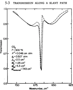
FIG. 5-3.5. Comparison of the transmission of carbon dioxide in the 15-μ region measured by Howard et al.⁹⁶ (solid curves) and computed by using the random-Elsasser band model (dashed curves).

850 900 ^{950 1000}

Wavenumber, cm"¹ 1050 1100

FIG. 5-3.6. Temperature dependence of the transmission of the 9.4- and 10.4-/X bands of carbon dioxide observed by Burch et al.¹³⁷ (solid curves) and computed by using the random-Elsasser band model (dashed curves).

2 4 8 5. ATMOSPHERIC TRANSMISSION

0

0.1

0.2

0.3

z 0.4

g (/>

(/>

2 0.5

(/) z

<

tr H 0.6

0.7

0.8

0.9

1.0

2100 2150 2200 2250 2300 WAVENUMBER, cm-·

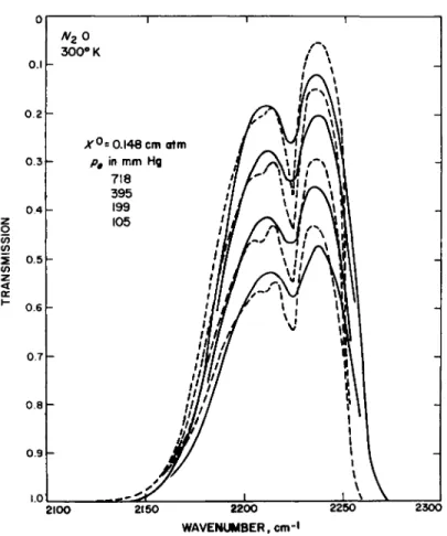
FIG. 5-3.7. Comparison of the transmission of nitrous oxide in the 4.6-μ, region measured by Burch and Williams¹⁶¹ (solid curves) and computed by using the random- Elsasser band model (dashed curves).

χο^ o = 0.22 cm-atm, and Xg0 = 0.06 cm-atm, where the superscript 0 indicates standard conditions of temperature (T = 273°K) and pressure (p = 1 atm). One of the principal difficulties in using an equivalent homogeneous path involves the determination of a suitable average temperature. It has been found that reasonably good agreement with experimental observations may be obtained by employing a "pressure- weighted" average temperature. That is, for a given sounding (tempera- tures at various pressure levels), the estimate T = ZTkpk\Zpk is a suitable average temperature. There is no theoretical justification for the use of this relation. Nevertheless, the results shown in Fig. 5-3.9 (points

Nz0 300° K

Γ

T

X°= 0.148 cm atm j h pê in mm

718 395

L 199 105

Γ

— <*

Hg

4

if A ill 11

ill ilj

ill

ill I Ml / '// f 1

II t

ll ] j l\ 7 / i l\iIn

'II·/

1 l·/

1

In

1 >/

ijf

Ί

f / /

¥

jr-*± at

i Mr

x-v I If x x * Ί

f ^χ%ιιΓ

h *M'/

r

\ 1/

\!

j

1

\

■OV

Λ4ι

*\ \\

v * 11 v it

Mil

Mil

\ fill

«W \\

111 I l u 1

111 1 vjl 1

■\ 1

1\

\ M i 1 i 1 \ 1

\ \ \ \

I \ \ \ \ -

-

_

Ί

H

5-3 TRANSMISSION ALONG A SLANT PATH 249 labeled one-level sounding) agree well with much more accurate calcula- tions (points labeled ten-level soundings).

To determine the transmission between various levels in an inhomo- geneous atmosphere, the Curtis-Godson¹⁹³'¹⁹⁴ approximation was used.

Thus a mean value SX° is defined for each vibrational transition at each frequency by the relation

SX° Sds°;

J n (5-3.18)

a mean rotational line half-width is similarly defined as

cx Sbds°

cx Sds°

J n

(5-3.19)

2000 2100 2200 2300 WAVENUMBER, cm"¹

2400

FIG. 5-3.8. Homogeneous path transmission for the atmosphere of the earth, from 4.3 to 4.8 μ. The calculations refer to one air mass, and the upper curve corresponds to the transmission from the surface to the top of the atmosphere; the lower curves correspond to the transmission from various heights in the atmosphere to the top of the atmosphere. Reproduced from Gray and McClatchey.¹⁸²

250 5 . ATMOSPHERIC TRANSMISSION

g ω

V) S (/) z

<

OC

1.0

0.9^

0.8

0.7

0.6

0.5

0.4

0.3

0.2

0.1

0

1 —

^ν κ \

A

- A

u

- -

1

— ι r ^{— i 1 1}

RECORD No. 41 OF LOW RESOLUTION MURCRAY DATA:

ZENITH ANGLE * 65°

—

% \

1 L

- -

X

O

P « 245 mb

EXPERIMENTAL CALCULATED 10 LEVEL SOUNDING 1 LEVEL SOUNDING

— I 1 > < Γ ^

—\

-\

H

-\

À

-\

A

2180 2200 2220 2240 2260 2280 WAVENUMBER, cm"¹

2300 2320

FIG. 5-3.9. Comparison of computed transmission (dashed curve), for a ten-level atmospheric sounding and for an ''equivalent*' isothermal atmosphere, with experimental¹³⁶ observations (solid curve).

Kaplan¹⁹⁵ has shown that this approximation yields the correct transmis- sion in both the limits of weak absorption and of strong absorption, and produces only a small error for intermediate values. T h e integrals in Eqs. (5-3.18) and (5-3.19) may be expressed in terms of generalized exponential integrals;¹⁹⁵ in the calculations, a computer subroutine due to R. H. Norton was used in which the required En functions (including nonintegral values of n) were directly computed.

T o summarize, the transmission for each vibrational transition was obtained from Eq. (5-3.6) by using the average values of ß and x obtained from Eqs. (5-3.18) and (5-3.19) for a particular frequency. T h e total transmission was then found by forming the product of the individual

5-3 TRANSMISSION ALONG A SLANT PATH 251 transitions according to Eq. (5-3.1). The transmissions computed from the Curtis-Godson approximation and observed during a balloon flight¹³⁶ are shown in Figs. 5-3.9 and 5-3.10; the spectral agreement is seen to be quite good. Similar calculations have been made by Plass¹⁸¹ for C 02 absorption only. It is apparent that N20 and CO must be included in calculations of atmospheric transmission in the 4.3-μ region.

Figure 5-3.11 shows the computed atmospheric transmission for the 2-μ region, assuming an isothermal path, as well as the experimentally observed transmission. The effect of various temperature and pressure distributions on the transmission of a single rotational line that is both Doppler- and pressure-broadened is illustrated in Fig. 5-3.12. The transmissions were computed for two normal traversais of a "Martian"

atmosphere, i.e., surface pressures of 5 and 10 mb and surface tempera- tures of 230 and 250°K were used, with an adiabatic lapse rate assumed in the lowest scale height of the atmosphere and a constant temperature of 185°K above that level. The calculations were performed for a line in the "hot" band at 10.4 μ with a C 02 abundance of X° = 85 m-atm, and an average molecular weight for the atmosphere of 44. The line

CALCULATED EXPERIMENTAL

(MURCRAY ET AL)

RECORD No. 81 p - 18.6 mb 0 = 47.4deg

2180 2200 2220 2240 2260 2280 2300 2320 2340 2360 2380 2 4 0 0 WAVENUMBER, cm"¹

FIG. 5-3.10. Comparison of computed slant path transmission of the atmosphere (dashed curves) with measurements obtained from a balloon flight¹³⁶ (solid curves).

252 5. ATMOSPHERIC TRANSMISSION I.Op

0.9h O.Bh

O.7L- Z 0.6l·- O CO

i

CO z

<

0.3k

0.2K-

0.1 k

Ol I I I I 4700 4800 4900 5000 5100

WAVENUMBER, cnH

FIG. 5-3.11. Comparison of observations of transmission of the atmosphere of the earth in the 2-μ region (solid curve) with calculations for an "equivalent" isothermal atmosphere. The dashed curve was computed for a 25 c m^{- 1} triangular slit function and the dotted curve corresponds to 2 c m^{- 1} resolution; 77@ = number of air masses, Xco2 ⁼ amount of COz in one air mass.

profile shown in Fig. 5-3.12 is seen to be quite sensitive to the assumed values of surface temperature and pressure. McClatchey and Norton²³⁶ have suggested that scanning such a line with a C 02 laser on board a Mars-orbiting spacecraft would allow a determination of the surface pressure and temperature of the lower atmosphere of Mars.

5-4 Spectral distribution of the intensity of radiation emerging from a planetary atmosphere

Once the accuracy of transmission calculations has been established, the same approximations may be used, with some confidence, in com- puting the spectral distribution of radiation between any point in the atmosphere and space for a given temperature profile. The solution of

Γ*250^βΚ /^«eOOmb

* c o2s 2-0 5 m a t m

^©=1.05

5-4 SPECTRAL DISTRIBUTION OF THE INTENSITY 253

z o

2 </>

z <

a: \-

1.0 0.9 0.8 0.7 0.6 0.5 0.4 0.3 0.2 0.1 0

I — T - 1

\ ^S \ \

" \ \V

N\ \\ M

N \\

* M * ^v

\ * \

\ \ \ \

10.4/A C02 \ P(24) \

\

1 » '

— i 1 r

p = 5 mb — y Γ = 230°Κ

\ P - 5 mb — '

\ 7" = 250^eK

M l / \\ \ /

1

V //

* \ /

1 "* τ ^ ι

1 " — — J - - : ^ ^

/ / '' '* 1

/ / ' ''

/ / / •

"7 // '' ^

H' /

7 / ' />·—/> = IOmb

/ L/, ^Γ=230·Κ

/' / // / /' /

f 1 t '

1

f ,L^—P = IOmb

^ Γ = 250 ^eK 1 /

1 1 1 1

1 _

1 1 1 0.005 0004 0.003 0.002 OXXX 0 0.001 0002 0.003 0.004 0.005

|ω-ω0|, cm"¹

FIG. 5-3.12. Effect of assumed model atmospheres on the transmission of an individual rotational line, computed for a Martian atmosphere.²³⁶

this problem requires solution of the equation of radiative transfer.²³⁷'*

In practice, it is necessary to assume local thermodynamic equilibrium (LTE) and to neglect scattering. This last assumption is well justified for the atmosphere of the earth in the infrared region of the spectrum where scattering is unimportant; however, it is a poor approximation for the visible region of the spectrum.

The equation of transfer is (see Chapter 2 for details)

dIM ΡωαΧ(Ιω-Βω), (5-4.1) where Ιω is the monochromatic intensity of radiation and Βω is the blackbody steradiancy. Equation (5-4.1) has the formal solution [cf.

Eqs. (2-1.21) and (2-1.22)]

I{X) = B(Tg) r(g, X) + \^X B(T.) τ(ί, X) P ds, (5-4.2)

J a

* See Chapter 2, and especially Section 2-1, for a detailed discussion of radiative transfer theory.

254 5. ATMOSPHERIC TRANSMISSION

where

r(g)X) = exp(-fpds)

and we have omitted the subscript ω for brevity. According to Eq. (5-4.2), the intensity of radiation observed at an optical depth X in the atmos- phere is equal to the intensity of blackbody radiation emitted by the ground (subscript g)> multiplied by the transmission from the level g to the level X, plus the intensity of radiation emitted by the distributed gases in the atmosphere (which are optically thin and have an emissivity of P ds), multiplied by the transmission from the level s to the level X.

We may rewrite Eq. (5-4.2) as

I(X) = B(rg) r(gy X) 4- C B{TS) dr, (5-4.3)

J r(g,X)

where we regard the transmission τ as the variable of integration. At a particular frequency, the transmission is a function of temperature and hence the Planck function may be written as a function of the trans- mission. This result is not immediately obvious because the transmission is known to be a function of pressure and optical depth, as well as of temperature. However, the assumption of a uniform mixing ratio yields a simple relation between pressure in the atmosphere and the optical depth. Hence, assuming a constant temperature lapse rate between specified pressure levels, we obtained a relation between pressure and temperature, viz.,

(TT/TS) = {prip&yy (5-4.4) where κ = (J7?g/g), Γ is the temperature lapse rate, Rg is the specific gas

constant for dry air, and g is the acceleration of gravity. Once Β(τ) is known for a particular frequency, the integral in Eq. (5-4.3) may be evaluated numerically. Figure 5-4.1 shows B(r) as a function of τ for several frequencies. The areas under these curves represent the inten- sities reaching the 200-mb level from the terrestrial atmosphere below that level, for the temperature soundings shown in Fig. 5-4.2. Figure 5-4.3 shows the calculated intensity of radiation passing upward through the 49-mb level of a seven-level atmospheric sounding, and also shows the blackbody curves for various temperatures of the sounding. It is seen that the radiation intensity approaches that of a blackbody, the temperature of which is that of the upper level of the sounding in the center of the P-branch (where the absorption is strong) and that of a blackbody with temperature equal to that of the lower level of the sounding in the wings of the bands (where the absorption is weak).

5-4 SPECTRAL DISTRIBUTION OF THE INTENSITY 255 2.4

2.2 2.0

18 16 1.4

1

K- 1.2 1.0 0.8 0.6 0.4 0.2 0

0 0.1 0.2 0.3 0.4 0.5 0.6 0.7 0.8 0.9 1.0 TRANSMISSION,!—*

FIG. 5-4.1. The Planck blackbody function plotted as a function of transmission for various frequencies. The areas under the curves correspond to the integration specified in Eq. (5-4.3). Reproduced from Gray and McClatchey.¹⁸²

The preceding calculations indicate that a basic problem of interest to meteorologists involves the intensity distribution (or transmission of the atmosphere), the temperature sounding that is consistent with the observed intensity distribution, and the question of uniqueness of the results.

It is apparent that a successful atmospheric temperature sounding by spectroscopic means from a satellite or space probe requires the use of a molecular absorption band located in the region of the planet-atmosphere system. In order to avoid solving the equations of radiative transfer for combined solar radiation and thermal radiation of the atmosphere, it is necessary to use the infrared region of the spectrum and wavelengths greater than about 4 μ (see Fig. 1.1 of Goody¹). In addition, the absorp- tion band must belong to a species the concentration of which is constant in the planetary atmosphere, i.e., the number density of molecules is a

L

\

ω=22

\

\

\

6 0 cm

ω = 22<

-1

30 cm^- 300 cr

-1 n""¹

- ω = 2 220 er Ί - l

v»^

256 5. ATMOSPHERIC TRANSMISSION

unique function of pressure. In this case, the measurement will deter- mine the atmospheric temperature as a function of pressure.^238-250

Of the minor constituents of the atmosphere that are known to be uniformly mixed, carbon dioxide is the most abundant. Kaplan has suggested²³⁹ that the 15-μ, bands, which are located near the maximum of the blackbody radiation curve for 300°K, would be particularly useful for sounding the atmosphere of the earth. However, the present state- of-the-art for infrared detector sensitivity is such that measurements can be made in either the 15- or 4.3-μ, C 02 bands with comparable instrumen- tal signal strength. There are many instrumental difficulties involved in measuring radiation near 15 μ that are not present at the shorter wave- lengths and this fact, coupled with the greater sensitivity of the 4.3-/x bands to variations in temperature, suggests that it is preferable to con- duct the experiment at 4.3 /x. The Planck function is well approximated

I0| , , , , , , , , ,

20h

30l·

5 0 h 70l·

E

« look

200l·

300h

500h 700h IOOOL

20Q 2K> 220 230 240 250 260 270 280 290 300 Temperature, °K

FIG, 5-4.2. Seven-level temperature sounding, used in computing the intensity distribution shown in Fig. 5-4.3.